Approximate Measurement Invariance of Willingness to Sacrifice for the Environment Across 30 Countries: The Importance of Prior Distributions and ...
←
→
Page content transcription
If your browser does not render page correctly, please read the page content below
ORIGINAL RESEARCH
                                                                                                                                                    published: 22 July 2021
                                                                                                                                          doi: 10.3389/fpsyg.2021.624032

                                                Approximate Measurement
                                                Invariance of Willingness to Sacrifice
                                                for the Environment Across 30
                                                Countries: The Importance of Prior
                                                Distributions and Their Visualization
                                                Ingrid Arts*, Qixiang Fang, Rens van de Schoot and Katharina Meitinger

                                                Department of Methodology and Statistics, Faculty of Social Sciences, Utrecht University, Utrecht, Netherlands

                                                Nationwide opinions and international attitudes toward climate and environmental
                                                change are receiving increasing attention in both scientific and political communities.
                                                An often used way to measure these attitudes is by large-scale social surveys. However,
                                                the assumption for a valid country comparison, measurement invariance, is often not
                                                met, especially when a large number of countries are being compared. This makes
                           Edited by:
                                                a ranking of countries by the mean of a latent variable potentially unstable, and may
               Alexander Robitzsch,
IPN—Leibniz Institute for Science and           lead to untrustworthy conclusions. Recently, more liberal approaches to assessing
   Mathematics Education, Germany               measurement invariance have been proposed, such as the alignment method in
                         Reviewed by:           combination with Bayesian approximate measurement invariance. However, the effect of
                         Niki De Bondt,
        University of Antwerp, Belgium          prior variances on the assessment procedure and substantive conclusions is often not
                        Artur Pokropek,         well understood. In this article, we tested for measurement invariance of the latent variable
 Institute of Philosophy and Sociology
                                                “willingness to sacrifice for the environment” using Maximum Likelihood Multigroup
                          (PAN), Poland
                                                Confirmatory Factor Analysis and Bayesian approximate measurement invariance, both
                   *Correspondence:
                             Ingrid Arts        with and without alignment optimization. For the Bayesian models, we used multiple
                       i.j.m.arts@uu.nl         priors to assess the impact on the rank order stability of countries. The results are
                                                visualized in such a way that the effect of different prior variances and models on group
                   Specialty section:
         This article was submitted to          means and rankings becomes clear. We show that even when models appear to be
         Quantitative Psychology and            a good fit to the data, there might still be an unwanted impact on the rank ordering
                        Measurement,
               a section of the journal
                                                of countries. From the results, we can conclude that people in Switzerland and South
               Frontiers in Psychology          Korea are most motivated to sacrifice for the environment, while people in Latvia are less
         Received: 30 October 2020              motivated to sacrifice for the environment.
           Accepted: 21 June 2021
                                                Keywords: measurement invariance, visualization, Bayes, group ranking, MGCFA, prior sensitivity, Bayesian
           Published: 22 July 2021
                                                approximate measurement invariance (BAMI)
                               Citation:
 Arts I, Fang Q, van de Schoot R and
      Meitinger K (2021) Approximate
            Measurement Invariance of
                                                INTRODUCTION
         Willingness to Sacrifice for the
   Environment Across 30 Countries:
                                                One of the main issues the world population faces today is climate and environmental change. Some
 The Importance of Prior Distributions          of the challenges that have to be faced include floods, droughts, food insecurity, and biodiversity
                 and Their Visualization.       loss. These challenges may give rise to socioeconomic problems such as refugee crises, relocating
           Front. Psychol. 12:624032.           populations and cities, and famines (Zhang et al., 2020). As the challenges will differ across regions,
    doi: 10.3389/fpsyg.2021.624032              but are not limited by national borders, international cooperation is required. At the same time,

Frontiers in Psychology | www.frontiersin.org                                          1                                             July 2021 | Volume 12 | Article 624032
Arts et al.                                                                                                  Measurement Invariance: Priors and Visualization

a “one size fits all” solution is unlikely to solve these issues           holds is usually done by conducting a maximum-likelihood
(Andonova and Coetzee, 2020). Several studies have been                    (ML) Multi-Group Confirmatory Factor Analysis (MGCFA).
conducted on how the inhabitants of different countries perceive           There are at least four types of MI: configural (also referred
the subject of climate and environmental change, and the                   to as “weak”), metric, scalar (“strong”), and residual (“strict”)
different aspects of social behavior regarding this subject: e.g.,         invariance. Configural invariance allows for the comparison of
knowledge of climate change, risk perception, and the willingness          latent variables among groups, metric invariance allows for a
to act (van Valkengoed and Steg, 2019). Hadler and Kraemer                 comparison of the items (questions) that make up the latent
(2016) showed that the inhabitants of different countries do not           variable(s) among groups, and scalar invariance allows for the
assess all these threats in the same way: in some countries air            comparison of latent means across groups. Scalar invariance,
pollution is seen as a major threat, while in others water shortages       however, is rarely established, especially when many groups are
are considered a hazard.                                                   compared (e.g., Muthen and Asparouhov, 2013; Lommen et al.,
    The term “environmental concern” has been used widely to               2014; Kim et al., 2017; Marsh et al., 2018)1 .
explain environmental behavior (e.g., Dunlap and Jones, 2002;                  Measurement invariance of the latent variable WTS has been
Bamberg, 2003; Schultz et al., 2005; Franzen and Meyer, 2010;              investigated by Mayerl and Best (2019), and they established both
Marquart-Pyatt, 2012a; Fairbrother, 2013; Pampel, 2014; Mayerl,            configural and metric invariance, but not scalar invariance. Using
2016; Pisano and Lubell, 2017; Shao et al., 2018). However, a              ML MGCFA, Marquart-Pyatt (2012b) also found configural and
clear definition of this concept is lacking (e.g., Dunlap and Jones,       metric invariance, but not scalar invariance. To our knowledge,
2002; Schultz et al., 2005). Bamberg (2003, p. 21) described               scalar invariance for the latent variable WTS has not been found
environmental concern as “the whole range of environmentally               by other authors, rendering the substantive interpretation of
related perceptions, emotions, knowledge, attitudes, values, and           results from country rankings potentially untrustworthy (Byrne
behaviors,” while Dunlap and Jones (2002, p. 485) described                and van de Vijver, 2017; Marsh et al., 2018).
environmental concern as “the degree to which people are aware                 Alternative approaches have been proposed, such as alignment
of problems regarding the environment and support efforts                  optimization, which allows for few but larger parameters
to solve them and/or indicate the willingness to contribute                differences between some groups (Asparouhov and Muthén,
personally to their solution.” Following the latter definition,            2014), Bayesian Approximate MI (Muthén and Asparouhov,
environmental concern consists of at least two parts: on the one           2012; van de Schoot et al., 2013), hereinafter referred to as
hand, perceptions of environmental problems (e.g., risks and               BAMI2 , which allows multiple but small differences between all
beliefs), and, on the other hand, the willingness to contribute to         groups, or a combination of both, BAMI alignment (Asparouhov
the solution (e.g., to pay more taxes or higher prices, or to fly          and Muthén, 2014). When BAMI alignment is used, small
less). This translates into two latent variables that operationalize       variances are allowed for each group, while a few groups are
environmental concern: “environmental attitude” (EA) and                   allowed to have large variances. This leads to fewer noninvariant
“willingness to sacrifice (or pay) for the environment” (WTS).             parameters than when the ML alignment method is applied,
These two latent variables have been used both individually and            facilitating the interpretation of the model (Asparouhov and
in combination to operationalize environmental concern (Mayerl             Muthén, 2014). Although this might be a highly interesting
and Best, 2019). The latent variable WTS is frequently used                approach when a comparison of many groups is desired, it
to measure the extent to which people are willing to sacrifice             seems that, at least up until now, this approach has not been
something in their daily life (money, goods, time, comfort) to             applied often: we only found two studies in which BAMI and
save the environment, and has been examined by several authors             alignment are combined: De Bondt and Van Petegem (2015)
(e.g., Ivanova and Tranter, 2008; Fairbrother, 2013; Franzen and           and van de Vijver et al. (2019), and certainly not in the field of
Vogl, 2013; Pampel, 2014; Sara and Nurit, 2014; Shao et al., 2018).        environmental change.
The relation with cultural, sociological, economic, or political               The key to using Bayesian methods is the use of priors:
factors has been studied quite extensively (e.g., Marquart-Pyatt,          some “wiggle room” is defined between which the variances of
2012b; Franzen and Vogl, 2013; Pampel, 2014; Bozonnet, 2016;               different groups are allowed to vary. However, the selection of
McCright et al., 2016; Shao et al., 2018).                                 these priors (from simulation studies, literature, or experience)
    Large-scale surveys are often used for exploring knowledge,
attitudes, and (intentional) behavior regarding climate and                1 Residual invariance means that the sum of specific variance (variance of the item
environmental change (e.g., Bamberg, 2003; Franzen and Meyer,              that is not shared with the factor and error variance) are also equal across groups
2010; Marquart-Pyatt, 2012a; Hadler and Kraemer, 2016; Knight,             (Putnick and Bornstein, 2016). Since this is not a requirement for comparing
2016; Pisano and Lubell, 2017; Libarkin et al., 2018). One                 means across groups, we do not report it in this article.
                                                                           2 In previous research, the term Approximate MI (van de Schoot et al., 2013) has
precondition for the valid comparison of attitudes toward                  sometimes been used as a collective term for any method that can be used when the
climate and environmental change across many countries is                  criteria for the exact scalar model are not fulfilled (Russell et al., 2016; Flake and
that measurement properties are equivalent across countries                McCoach, 2018), and sometimes to mention a specific method (e.g., Byrne and
(Jöreskog, 1971; Vandenberg and Lance, 2000). This means                   van de Vijver, 2017; Amérigo et al., 2020). To prevent any further confusion, we
that all participants in all countries should interpret both the           propose to use the term Bayesian Approximate Measurement Invariance (BAMI)
                                                                           when using a Bayesian model with strong informative priors on differences
survey questions and the underlying latent variables in the                between factor loadings and/or intercepts, thus excluding non-Bayesian (ML or
same way. This equivalence of measurement properties is also               empirical Bayes) type of methods like random item effects (Fox and Verhagen,
called Measurement Invariance (MI). Establishing whether MI                2018).

Frontiers in Psychology | www.frontiersin.org                          2                                                July 2021 | Volume 12 | Article 624032
Arts et al.                                                                                                        Measurement Invariance: Priors and Visualization

is not an easy task. It seems that researchers applying Bayesian                of ηig . For WTS let P = 3 (3 items) and G = 30 (30 countries),
methods are not always fully aware of the potential impact of                   which means that λpg is a 3 × 30 matrix. The same is true for νpg .
specifying priors (e.g., Spiegelhalter et al., 2000; Rupp et al., 2004;             In the configural model, both λ and ν are allowed to vary
Ashby, 2006; Kruschke et al., 2012; Rietbergen et al., 2017; van de             across groups3 , but the factor structure is equal for all groups,
Schoot et al., 2017; König and van de Schoot, 2018; Smid et al.,                that is, in all 30 countries the latent variable WTS is covered by
2020). Nonetheless, for the verification and reproducibility of                 the same three items.
research (Munafò et al., 2017; van de Schoot et al., 2021), it is                   When both the number of latent variables and the factor
crucial to evaluate the influence of varying priors on the impact               loading λ are held equal across groups but the intercept ν is
of substantive conclusions, which is referred to as sensitivity                 allowed to vary, one is testing for metric invariance: λ11 = λ12 =
analysis. Some general guidelines regarding prior sensitivity can               λ13 , etc. This means that for every group, the latent variable ηg
be found in the literature (e.g., Depaoli and van de Schoot, 2017;              contributes equally to item ypg .
van Erp et al., 2018; van de Schoot et al., 2019; Pokropek et al.,                  If metric invariance holds, it is possible to test for scalar
2020). Although a sensitivity analysis of different prior settings              invariance. In this case both loadings λ and intercepts ν are held
helps to determine the impact of prior variances on substantive                 equal across groups: λ11 = λ12 = λ13 etc. and ν11 = ν12 = ν13
conclusions, it has, to our knowledge, never been applied for                   etc., so that Equation (1) becomes:
BAMI with empirical data.
   The goals of our article are to apply the method of BAMI to the
concept of “willingness to sacrifice (or pay) for the environment,”                                          yp = νp + λp η + ǫipg                                 (2)
compare the results of different prior settings to each other and to
other methods of dealing with measurement invariance (i.e., ML                  When scalar invariance holds, the latent means of WTS can be
MGCFA and the ML alignment method) through visualization,                       compared between groups, and a ranking of the latent means
and to provide an example for a transparent workflow.                           can be made. However, scalar, or strong, invariance is very
   In what follows, we first provide a technical introduction to                rare, especially when comparing many groups (Asparouhov and
the four methods we used to assess MI. As it can be difficult to                Muthén, 2014; Byrne and van de Vijver, 2017; Kim et al., 2017;
interpret multiple models and methods, and because we want                      Marsh et al., 2018). This is due to the fact that with increasing
to be as transparent as possible in our decision-making process,                number of countries, the probability increases that countries
we summarize our design choices and possible alternatives in a                  substantially deviate in answering behavior. When many groups
decision tree. We test the models to evaluate whether and how                   with small deviations are being compared, these small deviations
different prior variances influence the ranking of the countries                add up to the non-invariance of the scale assessing WTS.
on the latent variable WTS. We visualize the results to facilitate a
comparison of the latent means of different models and methods                  Alignment Optimization
without the use of complex and elaborate tables. All appendices,                To reduce the impact of a lack of measurement invariance
the scripts to reproduce our results, the final output files and                for many groups, the alignment optimization method has been
additional material can be found on website of the Open Science                 introduced (Muthen and Asparouhov, 2013; Asparouhov and
Framework (OSF) (Arts et al., 2021).                                            Muthén, 2014). Alignment optimization consists of two steps
                                                                                (Asparouhov and Muthén, 2014). First, a null model M0 is
TECHNICAL BACKGROUND                                                            estimated with loadings and intercepts allowed to vary across
                                                                                groups. As loadings and intercepts are freed across groups, factor
In this section, we introduce the four methods we used to evaluate              means and factor variances are set to 0 and 1 for every group:
measurement invariance: (1) ML MGCFA, (2) ML MGCFA                              αg = 0 and ϕg = 1. Now, the latent variable for the null model
using the alignment optimization, (3) BAMI, and (4) BAMI in                     ηg0 can be calculated.
combination with the alignment method.                                              Second, the method divides groups G into pairs Q and tries to
                                                                                find, for every Q, the intercepts and loadings that yield the same
MGCFA                                                                           likelihood as the M0 model (Asparouhov and Muthén, 2014;
The MGCFA model is defined as:                                                  Flake and McCoach, 2018). Now, λpg and νpg can be calculated,
                                                                                where αg and ϕg have to be chosen in such a way that they
                                                                                minimize the amount of measurement non-invariance and q1,
                         yipg = νpg + λpg ηig + ǫipg                 (1)        q2, etc. are the different pairs of groups in the data. For the
                                                                                full set of equations, see Asparouhov and Muthén (2014), Flake
where p = 1, ...P is the number of observed indicator variables,                and McCoach (2018). This means that, for the latent variable
g = 1, ...G is the number of groups, i = 1, ...N is the number                  WTS, q = 1...435 for every item (for every item there are 435
of individual observations, λpg is a vector of factor loadings, νpg             possible pairs).
is a vector of intercepts and ηig is a vector of latent variables.
Furthermore, ǫipg is a vector of error terms that is assumed to be              3 Technically speaking, this is not entirely correct: for identification of the model,
normally distributed with N(0, θpg ), and ηig is assumed to have a              Mplus by default fixes the loading/intercept of the first item of every group to 1. For
distribution of N(αg , ϕg ). θpg is the variance of ǫipg , αg is the mean       more details about parameterization of CFA models we refer the interested reader
of normally distributed latent variable ηig , and ϕg is the variance            to Little et al. (2006).

Frontiers in Psychology | www.frontiersin.org                               3                                                 July 2021 | Volume 12 | Article 624032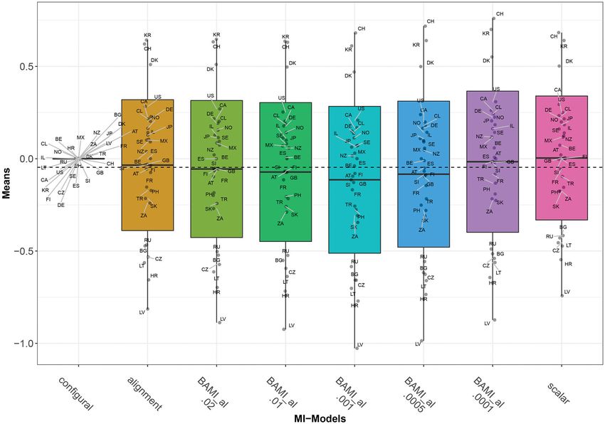
Arts et al.                                                                                                 Measurement Invariance: Priors and Visualization

   The total amount of measurement non-invariance is shown by                    BAMI
the total loss/simplicity function F:                                            A synopsis of Bayesian statistics, including the most important
                                                                                 aspects of determining prior distributions, likelihood functions
                       X X                                                       and posterior distributions, in addition to discussing different
                F =                 wg1 ,g2 f (λpg1 ,q1 − λpg2 ,q1 )             applications of the method across disciplines can be found in
                         p g1
Arts et al. Measurement Invariance: Priors and Visualization
the BAMI parameters and Equations (8) and (9), the configural TABLE 1 | Exact wording of the questions in WTS.
loadings and intercepts are computed for every iteration. These
Number Question
are then used to form the posterior distribution for λpg,0 and νpg,0 .
In the third and final step, the aligned estimates are obtained Q12a How willing would you be to pay much higher prices
for every iteration using the configural factor loading and in order to protect the environment?
intercept values to minimize the simplicity function of Equation Q12b How willing would you be to pay much higher taxes
(3). The aligned parameter values obtained from one iteration are in order to protect the environment?
used as starting values in the next iteration. Finally, the aligned Q12c How willing would you be to accept cuts in your
parameter values from all iterations are then used to estimate standard of living in order to protect the
environment?
the aligned posterior distribution as well as the point estimates
and the standard errors for the aligned parameters (Asparouhov
TABLE 2 | Participating countries in the ISSP environmental module.
and Muthén, 2014). This leads to fewer non-invariant parameters
than when the ML alignment method is applied, facilitating the Country Sample size Country Sample size
interpretation of the model (Asparouhov and Muthén, 2014).
Argentina 1,130 Lithuania 1,023
Australia 1,946 Mexico 1,637
METHODS AND DATA
Austria 1,019 Netherlands 1,472
Data Belgium (Flanders) 1,142 New Zealand 1,172
We used the data from the 2010 Module on Environment of the Bulgaria 1,003 Norway 1,382
ISSP (ISSP Research Group, 2019). For the full report on this Canada 985 Philippines 1,200
module, see GESIS (2019). The latent variable WTS consists of Chile 1,436 Portugal 1,022
three questions, see Table 1 for the exact wording, with answers Croatia 1,210 Russia 1,619
on a five-point response scale (1 being very unwilling and 5 Czech Republic 1,428 Slovakia 1,159
being very willing) and a cannot choose option for participants Denmark 1,305 Slovenia 1,082
who could not or would not answer the question. WTS has, Finland 1,211 South Africa 3,112
in combination with EA, been tested for MI by Mayerl and France 2,253 South Korea 1,576
Best (2019) to explain the concept “environmental concern” Germany 1,407 Spain 2,560
when applied to 30 countries: Austria, Belgium, Bulgaria, Great Britain 928 Sweden 1,181
Canada, Chile, Croatia, Czech Republic, Denmark, Finland, Iceland 798 Switzerland 1,212
France, Germany, Great Britain, Israel, Japan, Latvia, Lithuania, Israel 1,216 Taiwan 2,209
Mexico, New Zealand, Norway, Philippines, Russia, Slovakia, Japan 1,307 Turkey 1,665
Slovenia, South Africa, South Korea, Spain, Sweden, Switzerland, Latvia 1,000 United States 1,430
Turkey, and the United States. They found that, although metric
invariance was achieved, scalar invariance was not. When we Total 50,437
repeated this analysis we came to the same conclusion, for the
results of this analysis, see Appendix A in Arts et al. (2021). For
simplicity reasons, we only focus on the latent variable WTS, just
like Ivanova and Tranter (2008), Fairbrother (2013), Franzen and ensured that any differences in outcomes are due to a method and
Vogl (2013), Pampel (2014), Sara and Nurit (2014), and Shao not due to a difference in default settings of the model (for some
et al. (2018). To further analyze this scale, we first ensured that models by default the parameters are fixed for the first group,
we used the exact same data from the ISSP 2010 environment while for other models it is the last group). We selected Spain as
module and we followed the identical procedure as in the the reference country since the results presented by Mayerl and
original study to handle missingness (i.e., listwise deletion— Best (2019) indicate that the results for WTS from this country
correspondence with author, November 26 2019), resulting in the can be seen as “average” within the group of thirty countries.
same sample (n = 24,583). For the exact procedure and all code, For the BAMI method, both with and without alignment, we
see Appendix A in Arts et al. (2021). The sample sizes per country tested the effect of different priors on the models. One way of
ranges from 798 (Iceland) to 3,112 (South Africa) with an average selecting priors for new data is by using the results of simulation
group size of 1,401, see for more details Table 2. studies. Table 3 shows an overview of simulation studies that
have investigated BAMI and the priors that were used. As can
Analytical Strategy be seen from this table, the simulation results are not entirely
We assessed the measurement invariance of the latent variable conclusive: The authors of these articles report that they achieve
WTS by applying four methods for detecting MI: ML MGCFA, the best results when using priors with a variance of 0.001,
the ML alignment optimization, BAMI, and BAMI with 0.005, 0.01, or 0.05. However, the number of groups, group
alignment optimization. For all analyses, one reference country sizes and invariance criteria in these studies vary, complicating
was selected for which the factor mean and factor variance are a comparison of the best performing prior variance(s).
held to 0 and 1, respectively (Spain). By fixing the mean and We also searched for empirical studies in which BAMI was
variance for a specific reference country for every model, it is applied to empirical data. In a total of 30 empirical studies,
Frontiers in Psychology | www.frontiersin.org 5 July 2021 | Volume 12 | Article 624032Arts et al. Measurement Invariance: Priors and Visualization
TABLE 3 | Simulation studies using Bayesian approximate measurement maximum and minimum number of iterations to 100,000 and
invariance. 40,000, respectively.
Article Number of Group size Prior Invariance For the analysis in this article, we used the software Mplus
groups variance criteria version 8.4 (Muthén and Muthén, 2019). The results were
analyzed using R version 6.3.2 (R Development Core Team, 2017)
Muthén and 40 500 0.10, 0.05, PPP and MplusAutomation version 0-7.3 (Hallquist and Wiley, 2018)
Asparouhov, 2012 0.01
was used for the exchange between the two programs. More
van de Schoot 2 1,000 0.50, 0.05, PPP, 95% CI
information about the analysis and the exact Mplus and R code
et al., 2013 0.01, 0.005,
0.0005 can be found in Appendix B on Arts et al. (2021).
Kim et al., 2017 25, 50 50, 100, 0.05, 0.001 DIC, PPP,
1,000 95% CI, BIC
Lek et al., 2018 2 50, 100, 0.10, 0.05, 95% CI Model Fit
200, 1000 0.01, 0.001 To assess model fit for ML MGCFA, the indices that are
Shi et al., 2017 2 500 0.10, 0.05, PPP, 95%CI most widely used are the χ 2 -value, root mean square error of
0.01 approximation (RMSEA), comparative fit index (CFI), Tucker-
Pokropek et al., 24 1500 0.10, 0.05, cor, RMSEA, Lewis index (TLI), and the standardized root mean square
2019 0.01, 0.005 95%CI
residual (SRMR) (Gallagher and Brown, 2013, p. 298). When
4, 24, 50 400, 1500, 0.05, 0.025, BIC, DIC, testing for configural invariance cutoff values of CFI ≥ 0.95,
Pokropek et al. 3,000 0.01, 0.005, PPP
(2020) 0.001, 0.000∗
TLI ≥ 0.95, RMSEA ≤ 0.06, and SRMR ≤ 0.08 have been
proposed by Hu and Bentler (1999). When checking for metric
∗A Bayesian model with a prior variance of 0 is the scalar model. and scalar invariance, relative fit indices are more useful than
PPP, posterior predictive p-value; DIC, deviance information criterion; 95% CI, 95%
credibility interval; cor, correlation; RMSEA, root mean square error of approximation; BIC,
absolute fit indices (Chen, 2007). These relative fit indices are
Bayesian information criterion. a comparison of configural with metric and metric with scalar
fit indices. Depending on these fit indices, the model for metric
invariance can be assumed to perform better or worse than the
there were 13 in which only one prior was used, and in eight model for configural invariance (and the same is true for metric
of these 13 studies, no specification was given as to why that and scalar invariance). For sample sizes above 300, 1RMSEA
specific prior was used. In the 17 studies where multiple priors ≤0.015 and 1CFI ≤0.01 or 1SRMR ≤0.03 indicate invariance
were tested, three did not provide any information on why these when moving from the configural to the metric model, and
priors were selected. The 14 other studies based the priors used 1RMSEA ≤0.015 and 1CFI ≤0.01 or 1SRMR ≤0.01 indicate
on Muthén and Asparouhov (2012), van de Schoot et al. (2013), noninvariance when moving from the metric to the scalar model
Asparouhov et al. (2015), or Seddig and Leitgöb (2018). For more (Chen, 2007).
information about these empirical studies and their variances see For the alignment method, fit indices have not been specified.
the additional material (Arts et al., 2021). The most frequently Muthen and Asparouhov (2014) propose that the results can
used prior variance in these studies is 0.01, followed by 0.05 as be considered trustworthy when no more than 25% of the
recommended by Muthén and Asparouhov (2012) and van de parameters are non-invariant. However, Kim et al. (2017) have
Schoot et al. (2013), respectively. However, other priors were argued that this way the degree and location of non-invariance
also included in the different sensitivity analyses, ranging from cannot be taken into account.
0.000000001 to 0.5. When BAMI is used, the model fit may be indicated by the
We decided to estimate five different models, with priors posterior predictive p-value (PPP-value). This value indicates
with a variance of 0.05–0.01 (decreasing at 0.01 per prior) and the ratio between the iterations for which the replicated χ 2
three models with priors with variances of 0.001, 0.0005, and value exceeds the observed χ 2 value (Pokropek et al., 2020).
0.0001. This includes the prior variances that are used most A PPP-value of 0.50 indicates perfect model fit; a value below
often in both simulation and empirical studies. Using such a 0.50 indicates an underfit of the model, and a value above 0.50
large number of priors should create a clear overview of the indicates an overfit. Furthermore, the 95% credibility interval
influence of different prior variances on the rank order stability (CI) should include 0, preferably with 0 in the middle of
of the countries when ranked on their latent factor means. the interval (Muthén and Asparouhov, 2012; van de Schoot
In addition to priors on the differences between loadings and et al., 2013). As PPP-values decline, the model fits the data
intercepts, there are also priors on other parameters, such as less well. However, a specific cutoff value at which the model
the residuals. However, we will not discuss these priors in this no longer fits the data is hard to determine. Muthén and
article and we relied on the Mplus default values which can Asparouhov (2012) suggest that models with PPP-values lower
be found in Muthén and Muthén (2019). To ensure that the than 0.10, 0.05, or 0.01. do not fit the data anymore. In the
chains reached their target distributions, we checked whether literature, PPP-values above 0.05 are often seen as an indication
all iterations after burn-in met the Gelman-Rubin criterion. for good model fit. A drawback of the PPP-value is that it
Therefore, we set the convergence criterion to a rather strict 0.01 might not identify a model with good fit correctly when using
instead of the default 0.05 (Muthén and Muthén, 2019) and the different priors with large sample sizes (Asparouhov and Muthén,
Frontiers in Psychology | www.frontiersin.org 6 July 2021 | Volume 12 | Article 624032Arts et al. Measurement Invariance: Priors and Visualization
2010, 2019; Hoijtink and van de Schoot, 2018; Hoofs et al., 0.005, 0.01, 0.05, and 0.1. Both De Bondt and Van Petegem (2015)
2018)4 . and van de Vijver et al. (2019) analyzed the alignment part of the
Recently, Bayesian versions of fit indices have been model by comparing, for each item, the intercepts and loadings
proposed: Bayesian RMSEA (BRMSEA), Bayesian CFI across paired groups. This can be a very laborious process when
(BCFI), and Bayesian TLI (BTLI) can be computed based multiple items and multiple groups are concerned. One could
on differences between the observed and replicated discrepancy also use the rule of thumb that, to obtain trustworthy results, no
functions (Liang, 2020). These Bayesian fit statistics have been more than 25% of the parameters can be invariant, as proposed
implemented in Mplus version 8.4, making it more convenient by Muthen and Asparouhov (2014).
to identify good model fit (Asparouhov and Muthén, 2019). The As shown above, there are many different criteria and cut-off
calculation of these fit indices is very similar to that of the fit values that provide insight into whether a model fits the data.
indices of an exact model, and therefore, the same cutoff values Since there are so many different indicators these cutoff values
can be used (Asparouhov and Muthén, 2019; Garnier-Villarreal should be treated with care: fit statistics can be influenced by,
and Jorgensen, 2020). This means that BCFI ≥ 0.95, BTLI ≥ 0.95, e.g., sample size or model complexity (Chen, 2007). Additionally,
and BRMSEA ≤ 0.06 indicate good model fit. However, just as having one indication of good model fit is not enough to conclude
with the ML models, a combination of cutoff values must be used that the model is a good fit to the data, and multiple fit statistics
to indicate good or bad model fit. Other criteria that are being may even contradict each other. This exact point was addressed
used to determine model fit are the BIC (Schwarz, 1978) and by Lai and Green (2016), who showed that RMSEA and CFI can
the DIC (Spiegelhalter et al., 2002). These information theoretic contradict each other. Even when there is sufficient evidence that
indices are less self-explanatory than the other fit indices: when a model is a good fit to the data, this does not necessarily mean
selecting the best performing model from a series of models that it is the best model.
(the model that fits the data best and is the least complex), the
model with the lowest BIC or DIC is preferred. This does not
mean that the model with the lowest BIC or DIC is a good fit RESULTS
to the data: it is simply preferable to models with a higher BIC MGCFA
or DIC. Asparouhov et al. (2015) stated that, when sample sizes The fit indices for the metric and scalar MGCFA are shown in
are large, coupled with a large number of observed indicators, Table 4. Since the configural model was saturated, the results are
DIC is preferable to BIC and Pokropek et al. (2020) concluded not shown here. Therefore, for the metric model we asses the
that DIC is a good indicator to identify the preferred prior mean absolute fit indices instead of the relative fit indices. The metric
and variance. On the other hand, Hoijtink and van de Schoot model shows good fit, with a CFI and TLI of 0.993 and 0.989,
(2018) stated that the DIC is not suitable for evaluating models respectively. With 0.069 the RMSEA value is above 0.06 but still
with small priors. This makes the use of the DIC as fit index below 0.08, indicating at least a reasonable fit. The fit indices
promising, but also shows that its value should be treated with for the scalar model all point to rejection of the scalar model:
care. At a minimum, DIC should always be combined with other 1RMSEA, 1SRMR and 1CFI are well above the cutoff values of
fit indices. 0.015, 0.01, and 0.01 (0.085, 0.057, and 0.065, respectively). Based
BAMI with alignment has, similar to the ML alignment on these results we conclude that scalar invariance is absent, and
method, no guidelines to determine model fit. Both De Bondt that a comparison of the latent variable WTS across countries
and Van Petegem (2015) and van de Vijver et al. (2019) tested may not be trustworthy. However, this exact approach could be
a model with multiple small prior variances. De Bondt and Van too strict in its assessment.
Petegem (2015) used a prior variance of 0.01 and conducted a
sensitivity analyses with prior variances decreasing with a factor
10, and van de Vijver et al. (2019) used a prior variance of 0.05 Alignment Optimization
and conducted a sensitivity analyses with prior variances of 0.001, Regarding the alignment optimization, the invariant, and
non-invariant parameters are shown in Table 5 with non-
invariant parameters bolded and in brackets. Most non-invariant
4 Hoijtink and van de Schoot (2018) demonstrated that, with increasing sample parameters can be found in the intercepts, with 48 non-invariant
sizes, the PPP-value does not decrease, but increases. Therefore, the prior-posterior parameters, while for the loadings only seven parameters are
predictive p-value (PPPP-value) was proposed by Hoijtink and van de Schoot
(2018), and a generalized version was implemented in Mplus by Asparouhov
non-invariant. However, a total of 55 parameters are non-
and Muthén (2017). Whereas, the original PPP-value is a test of model fit which invariant, which is 30.55% of all parameters. This is well
tests the fit of the model to the data and is based on comparing the model with above 25%, a rough cut-off value proposed by Muthen and
the unrestricted covariance model, the PPPP-value is a test for the approximate Asparouhov (2014), implying that, for these data, a valid rank
parameters in the model. The PPPP-value is not a test for model fit and should not order comparison cannot be made if the ML alignment method
be interpreted as evidence that the model fits the data. The proper interpretation
of the PPPP-value is given by Asparouhov and Muthén (2017): “If the test does
is used.
not reject, the minor parameters (represented by θ1 ) can be assumed to come from
N(0, v) distribution, with v being a small variance. More broadly speaking, if the BAMI
PPPP does not reject, that means that there is no evidence in the data for the minor
parameters in model M(θ1 , θ2 ) to be outside the N(0, v) distribution” (p. 10). Here,
For BAMI, only the results for the models that converged are
θ2 represents the large parameters of model M. Unfortunately, the PPPP-value is presented here (models with a prior variance of 0.02, 0.01, 0.001,
not yet available for BAMI in Mplus. 0.0005, and 0.0001). These models also converged when the
Frontiers in Psychology | www.frontiersin.org 7 July 2021 | Volume 12 | Article 624032Arts et al. Measurement Invariance: Priors and Visualization
TABLE 4 | Fit statistics of the MGCFA model.
χ 2 (df) 1χ 2 (1 df) p-value RMSEA 1 RMSEA SRMR 1 SRMR CFI 1 CFI TLI 1 TLI
Configural*
Metric 287.324 (58) 0.00 0.069 0.051 0.993 0.989
Scalar 2382.434 (116) 2095.110 (58) 0.00 0.154 0.085 0.108 0.057 0.928 0.065 0.944 0.045
*This model was saturated. df, degrees of freedom; RMSEA, root mean square error of approximation; SRMR, standardized root mean square residual; CFI, comparative fit index; TLI,
Tucker-Lewis index. Numbers are absolute.
TABLE 5 | (Non)invariant parameters for ML alignment optimization.
Intercepts/Thresholds
Q12a 33 (40) (56) (100) (124) 152 191 203 (208) 246 (250) (276) (376) (392) (410) 428 440 484
(554) (578) (608) 643 703 705 710 752 (756) 792 (826) (840)
Q12b 33 40 56 (100) 124 (152) (191) (203) 208 246 250 276 376 392 410 (428) (440) (484) 554
578 (608) (643) (703) 705 (710) (752) 756 (792) (826) (840)
Q12c 33 (40) 56 (100) 124 (152) 191 (203) 208 (246) 250 276 376 (392) (410) (428) (440) 484
(554) 578 (608) 643 703 705 (710) (752) (756) (792) (826) (840)
Loadings
Q12a 33 40 56 100 124 152 191 203 208 246 250 276 376 392 410 428 440 484 554 578 608 643 703 705 710 752 756 792 826 840
Q12b 33 40 56 100 124 152 191 (203) 208 246 250 (276) 376 392 410 428 440 484 554 (578) 608 643 703 705 (710) 752 756 792 826 840
Q12c 33 40 (56) 100 124 152 191 203 208 246 250 276 376 392 (410) 428 440 484 554 578 608 643 703 705 710 752 (756) 792 826 840
Noninvariant parameters are in bold and within parentheses.
number of iterations was doubled, which was not the case for the From this figure it can be seen that with declining prior variance,
models with other prior settings. the outcome of the model approaches that of the scalar model (on
To select the model(s) with a good fit, one could use model the right). This is to be expected, as the scalar model is a model of
fit indices, but just as with regular SEM there is not one single priors with a mean and variance of 0.
statistic that should be used, and only a combination of fit indices Figure 2 is a graph of the means per country per model (scalar
should be used to indicate model fit. Table 6 shows fit statistics invariance, ML alignment, and all BAMI models). For illustrative
for the models with prior variances 0.02, 0.01, 0.001, 0.0005, and purposes, we present the results for BAMI both with and without
0.0001. Table 6 shows that only for models with a prior variance alignment in one figure. Figure 1 shows that the overall mean
of 0.02 and 0.01 the PPP > 0 (0.36 and 0.12, respectively) and differences between latent means of the different models are small
the 95% CI contains 0. BRMSEA is 0.014 for the model with a but increase as the prior variance decreases: 10.01−0.02 is 0.007
prior variance of 0.02, and it is 0.049 for the model with prior and 10.0005−0.0001 is 0.069. For individual countries, this is not
variance of 0.01. For the other models, BRMSEA > 0.1. For the always the case: Figure 2 shows that, for the 15 lowest ranking
model with prior variance 0.02, both BCFI and BTLI are 1.00, and countries this same pattern is visible, but for the top 15 countries
for the model with prior variance 0.01 BCFI is 0.999 and BTLI the means increase with prior variance. However, as the countries
is 0.994, indicating good model fit. Using PPP-value, the model rank lower, the differences between models increase. For the
with variance 0.02 comes closest to 0.5 with a PPP-value of 0.36. lowest-ranking country (Latvia) the difference between the model
However, the PPP-value might be untrustworthy because of the with prior variance 0.02 and that with prior variance 0.0001
large sample size of our study (24,583 respondents) (Asparouhov is 0.616, while for the highest-ranking country (Switzerland)
and Muthén, 2019). Hoijtink and van de Schoot (2018) stated the difference is 0.208. For the three highest-ranking countries
that the PPP-value is not suitable for evaluating small priors. (Switzerland, South Korea and Denmark) the model with the
Concerning both CI and BRMSEA, only the models with prior highest prior variance (0.02) shows larger differences from the
variances of 0.02 and 0.01 indicate a good fit. When looking model with a prior variance of 0.01 (0.173, 0.161, and 0.128,
at BCFI and BTLI, however, the models with prior variances respectively) than do other models with consecutively lower
of 0.02, 0.01, 0.001, and 0.005 all indicate good fit, although prior variances.
fit statistics approach to their cutoff values as prior variances
decline. When combining the above results with the DIC for the BAMI With Alignment
different models, the values for the model with prior variance 0.02 When the BAMI model with alignment is applied, first, the BAMI
is the lowest (19,7428.86), indicating that this is the best fitting model is estimated. The outcome of the BAMI models is given
model based on post-hoc fit indices. in the description above (Table 6). From this BAMI model, a
Figure 1 shows the means of the latent variable for the BAMI configural model is estimated, which is then aligned. This means
models with variances of 0.02, 0.01, 0.001, 0.0005, and 0.0001. that fit indices cannot be used to indicate model fit of the final
Frontiers in Psychology | www.frontiersin.org 8 July 2021 | Volume 12 | Article 624032Arts et al. Measurement Invariance: Priors and Visualization
TABLE 6 | Fit statistics of the BAMI models.
Prior
PPP 95% CI BRMSEA BCFI BTLI BIC DIC
variance
0.02 0.363 [−52.706 to 79.836] 0.014 1.000 1.000 200288.68 197428.66
0.01 0.117 [−25.495 to 109.968] 0.049 0.999 0.994 200324.54 197514.18
0.001 0.000 [669.517 to 852.222] 0.117 0.976 0.968 201095.93 198186.01
0.0005 0.000 [1100.629 to 1286.848] 0.130 0.962 0.960 201546.82 198601.39
0.0001 0.000 [1873.721 to 2022.907] 0.148 0.938 0.949 202327.90 199334.78
PPP, posterior predictive probability; CI, credibility intervals; BRMSEA, Bayesian root mean square error of approximation; BCFI, Bayesian comparative fit index; BTLI, Bayesian
Tucker-Lewis index; BIC, Bayesian information criterion; DIC, deviance information criterion.
FIGURE 1 | Means for configural invariance, scalar invariance, ML alignment, and BAMI models. AT, Austria; BE, Belgium; BG, Bulgaria; CA, Canada; CL, Chile; HR,
Croatia; CZ, Czech Republic; DK, Denmark; FI, Finland; FR, France; DE, Germany; GB, Great Britain; IL, Israel; JP, Japan; LV, Latvia; LT, Lithuania; MX, Mexico; NZ,
New Zealand; NO, Norway; PH, Philippines; RU, Russia; SK, Slovakia; SI, Slovenia; ZA, South Africa; KR, South Korea; ES, Spain; SE, Sweden; CH, Switzerland; TR,
Turkey; US, United States. The x-axis shows the different models—configural, scalar, ML alignment, and BAMI—with their specific variances. The dashed black line
shows the overall mean.
model. Instead, just as with the ML alignment model, we use all have a percentage of non-invariant parameters above 25%
the percentage of non-invariant parameters to determine good (although the model with prior variance 0.001 is only slightly
model fit. Table 7 shows the number of non-invariant parameters above), making the results, and thus a group ranking from
per model. these models, unreliable. For the models with prior variances of
From this table, it can be seen that, as prior variances 0.0005 and 0.0001 the percentages of non-invariant groups are
decrease, so does the number of non-invariant parameters. The 16.67 and 1.67, respectively, implying good model fit and a valid
three models with prior variances of 0.02, 0.01, and 0.001 group ranking.
Frontiers in Psychology | www.frontiersin.org 9 July 2021 | Volume 12 | Article 624032Arts et al. Measurement Invariance: Priors and Visualization
FIGURE 2 | Means per country for scalar invariance, ML alignment, and BAMI models with and without alignment. AT, Austria; BE, Belgium; BG, Bulgaria; CA,
Canada; CL, Chile; HR, Croatia; CZ, Czech Republic; DK, Denmark; FI, Finland; FR, France; DE, Germany; GB, Great Britain; IL, Israel; JP, Japan; LV, Latvia; LT,
Lithuania; MX, Mexico; NZ, New Zealand; NO, Norway; PH, Philippines; RU, Russia; SK, Slovakia; SI, Slovenia; ZA, South Africa; KR, South Korea; ES, Spain; SE,
Sweden; CH, Switzerland; TR, Turkey; US, United States. The x-axis shows the different models—scalar, ML alignment, and BAMI with and without alignment—with
their specific variances. Models that appear to ba a good fit to the data are indicated in bold green, models with bad fit in red.
TABLE 7 | The number of non-invariant parameters for the BAMI models with alignment.
Prior Number of non-invariant intercepts Number of non-invariant loadings Total number
Variance
Q12a Q12B Q12C Q12a Q12B Q12C Sum %
0.02 15 16 19 2 5 5 62 34.44
0.01 15 15 19 0 5 5 59 32.78
0.001 9 15 16 0 2 4 46 25.56
0.0005 4 11 12 0 1 2 30 16.67
0.0001 0 3 0 0 0 0 3 1.67
As with the ML alignment model, most non-invariant parameters are invariant for both models: Spain, Austria, Canada,
parameters are the intercept parameters. For the model with Denmark, Finland, Germany, Israel, Mexico, Russia, Slovakia,
the lowest number of non-invariant parameters (prior variance Slovenia, and Sweden. Figures 2, 3 show that, as the priors
0.0001), these parameters belong to the intercepts of question 12b decrease, so do the mean differences of the model outcomes (both
(are you willing to pay higher taxes to save the environment), for the overall means and the means per country).
the countries Lithuania, South Africa, and Turkey. When taking Figure 3 shows that for the first three models with decreasing
into account only the models with a percentage of non-invariant prior variance, the overall means also decrease. However, as
parameters below 25%, there are 12 countries for which all prior variances decrease further (0.0005 and 0.0001), they rise
Frontiers in Psychology | www.frontiersin.org 10 July 2021 | Volume 12 | Article 624032Arts et al. Measurement Invariance: Priors and Visualization
FIGURE 3 | Means for configural invariance, scalar invariance, ML alignment, and BAMI models with alignment. AT, Austria; BE, Belgium; BG, Bulgaria; CA, Canada;
CL, Chile; HR, Croatia; CZ, Czech Republic; DK, Denmark; FI, Finland; FR, France; DE, Germany; GB, Great Britain; IL, Israel; JP, Japan; LV, Latvia; LT, Lithuania; MX,
Mexico; NZ, New Zealand; NO, Norway; PH, Philippines; RU, Russia; SK, Slovakia; SI, Slovenia; ZA, South Africa; KR, South Korea; ES, Spain; SE, Sweden; CH,
Switzerland; TR, Turkey; US, United States. The x-axis shows the different models—configural, scalar, ML alignment, and BAMI with alignment—with their specific
variances. The dashed black line shows the overall mean.
slowly toward the means of the scalar model. The differences From Figure 2, we observe that there appear to be four different
between means of models with consecutive priors are less groups of countries with similar means: Switzerland, South Korea
clear than for the BAMI models (Figure 1). Now, 10.01−0.02 and Denmark at the top, then a large group with the United
0.016, 10.001−0.01 0.042, 10.0005−0.0001 0.0675, and 10.001−0.0005 States, Canada, Chile, Germany, Norway, Japan, Israel, Sweden,
0.031. Although this pattern is visible in the means per model New Zealand, Mexico, Austria, Great Britain, Finland, Spain,
(Figure 3), it is less distinctive when looking at the means of Slovenia, France, Turkey, Philippines, Slovakia, and South Africa.
individual countries (Figure 2). In that case, this pattern is most The third group comprises Russia, Czech Republic, Bulgaria,
pronounced for Latvia and, to a lesser extent, Bulgaria, Lithuania, Lithuania, and Croatia, while the bottom group consists of only
Hungary, Russia, South Africa, Slovakia, Turkey, the Philippines, one country: Latvia. In particular for the second group, means are
Denmark, Croatia, and Switzerland. Figures 2, 3 show that, as very close together, and it can be difficult to distinguish individual
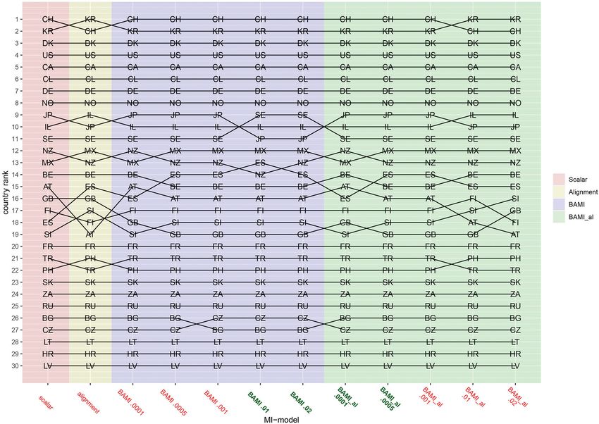
prior variances decrease, so do the mean differences of the country means. Figure 4 shows the ranking of the 30 countries
model outcomes (both the overall means and the means per for the analyzed models that converged. This figure shows that
country). Again, Latvia is the country with the most pronounced for nearly all the models, ranking changes somewhat when a
differences when comparing different priors. different prior variance is used. Upon closer inspection, 13 of
the 30 countries occupy the same place in the ranking for all
Ranking the models, and most changes appear to be in the middle of
Figures 1–3 show that the latent means vary depending on the the ranking. When combined with Figure 2, it becomes clear
choice of prior variance. Models with smaller prior variances that country mean differences are small, especially for the BAMI
seem to have outcomes that approach the outcome of the scalar model with alignment. For the BAMI models, country means
model. However, there is some variation at the country level. differ slightly more, especially at the top and the bottom of the
Frontiers in Psychology | www.frontiersin.org 11 July 2021 | Volume 12 | Article 624032Arts et al. Measurement Invariance: Priors and Visualization
ranking. Mean differences for Latvia decrease with decreasing differences would be or how many groups would differ
prior variance, and these differences are larger than the overall from each other, so we first followed the “yes” arrow to step
mean difference per model. 3 and tested for ML alignment.
Comparing the individual country means of the BAMI and
3. Does the alignment optimization yield < 25%
BAMI with alignment model shows that for all countries the
non-invariant parameters?
differences between the models decrease with prior variance:
differences between models are lowest when models with the a. Yes: The rank order can be trusted
lowest prior variances are compared. For the models with a prior b. No: Try another method to make means comparison valid.
variance of 0.0001 the country rankings are the same. Go top step 4.
Focusing on only the models that appear to have a good fit to This yielded > 25% non-invariant parameters, so we
the data, according to their fit statistics, only the BAMI models followed the “no” arrow to step 4.
with a prior variance of 0.02 and 0.01 and BAMI models with
4. Do you expect only small differences in parameters for
alignment with a prior variance of 0.0005 and 0.0001 are of
different groups6 ?
importance. When comparing the rankings of these models, the
ranking for the BAMI models is almost identical: only Spain and a. Yes: Only small differences. Use BAMI, Go to step 4A.
New Zealand switch places when changing models. The ranking b. No: Both small and large differences. Use BAMI in
of the BAMI models with alignment shows more variation: 23 combination with alignment optimization. Go to step 4B.
countries rank the same for both models, while Mexico, New Now, we had to decide whether we expected small or large
Zealand, Belgium, Austria, Great Britain, and Slovenia all shift differences in parameters for different groups. Since we did
one place up or down and Spain moves two places in the ranking. not know how large the differences per group were, we
These figures show that, regardless of prior variance or used both, as they lead to step 5 in this decision tree; which
even model fit, people in Switzerland and South Korea are option we chose would not make a difference.
most motivated to sacrifice for the environment, while people
in Bulgaria and Latvia are less motivated to sacrifice for 5. Then, we needed to decide which priors to use and run
the environment. the different models. We based our priors on previous
literature on the use of BAMI (both simulations and empirical
examples). We then moved to step 6.
Decision Tree
6. We visualized the outcomes of the different models [scalar, ML
As it can be difficult to draw conclusions from the means and
alignment, and BAMI models (with and without alignment)
rankings as shown in Figures 1–4, we devised a decision tree
that converged] in Figures 1–4 (means and group rankings).
(Figure 5). This tree provides some insight into the decisions
The code to create these Figures can be found in Appendix C
that we had to make regarding group means, group rankings and
on Arts et al. (2021). We moved to step 7.
the influence of priors. Based on this decision tree, other readers
7. Is the rank order as a whole stable? (Figure 4)
might come to different conclusions. The tree comprises the
entire process needed to evaluate the information contained in a. Yes: No or only minor changes in rank. Then the rank
Figures 1–4, starting with the MGCFA test for scalar invariance: order is not at all or only slightly influenced by the choice
of priors.
1. We started with an ML MGCFA test for scalar invariance. To
b. No: Many changes across groups and models. Go to step 8.
test for scalar invariance it is necessary that configural and
Since there were numerous changes in the rank order, we
metric invariance are met.
did not consider the rank order stable and we followed the
a. Yes: It is now possible to compare ranks. “no” arrow to step 8.
b. No: Try another method to make means comparison valid.
8. Does the pattern of the rank order across different models
Go to step 2.
make sense?
We did not find scalar invariance, so we followed the “no”
arrow to step 2. a. Yes: Many changes, but all changes in the same section of
the ranking (e.g., top) or the same groups change rank. Go
2. Do you expect a large difference in parameters for some
to step 9.
groups and equality for the rest of the groups5 ?
b. No: The pattern seems erratic. Go to step 10.
a. Yes: Equality for almost all groups. Go to step 3. From Figure 5 we concluded that the upper and the lower
b. No: Only small differences or small and large differences. parts of different rankings hardly change, and most rank
Go to step 4. changes take place in the middle part of the ranking.
We assumed there would be some differences in the We considered this a logical pattern and followed the
parameters, although we did not know how large these “yes” arrow.
5 When in doubt whether large difference in parameters for some groups are to be 6 Similarly, when in doubt whether small differences for many groups are to be
expected, it is advisable to consult a substantive expert of your field. The decision expected, it is advisable to consult a substantive expert of your field. The decision
whether large parameters can be expected should be based on previous research whether small parameter differences can be expected should be based on previous
and/or expertise. research and/or expertise.
Frontiers in Psychology | www.frontiersin.org 12 July 2021 | Volume 12 | Article 624032Arts et al. Measurement Invariance: Priors and Visualization
FIGURE 4 | Rankings per model. AT, Austria; BE, Belgium; BG, Bulgaria; CA, Canada; CL, Chile; HR, Croatia; CZ, Czech Republic; DK, Denmark; FI, Finland; FR,
France; DE, Germany; GB, Great Britain; IL, Israel; JP, Japan; LV, Latvia; LT, Lithuania; MX, Mexico; NZ, New Zealand; NO, Norway; PH, Philippines; RU, Russia; SK,
Slovakia; SI, Slovenia; ZA, South Africa; KR, South Korea; ES, Spain; SE, Sweden; CH, Switzerland; TR, Turkey; US, United States. The x-axis shows the different
models—scalar, ML alignment, and BAMI with and without alignment—with their specific variances. Models that appear to ba a good fit to the data are indicated in
bold green, models with bad fit in red.
9. Are individual groups stable across models? b. No: Do not use rank order.
Figure 3 shows that the differences per group are quite
a. Yes: Individual groups never move more than one place up
small, especially in the middle part of the ranking where
or down in the ranking across different models. Then the
most changes in rank take place. We therefore conclude
rank order is not or only slightly influenced by the choice
that there is almost no difference between groups.
of priors
b. No: Individual groups continue moving up or down the
ranking across different models. CONCLUSION AND DISCUSSION
Changes in rank nearly always applied to the same
The latent variable “willingness to sacrifice for the environment”
countries, making the pattern rather stable. However, as
(WTS) is an important aspect of environmental concern. It
some countries moved up or down two or three positions
can provide insights into the intentional behavior regarding
in the ranking across models, we found that stability of
the groups could not be guaranteed. We followed the environmental concern, which, in turn, provides more insight
“no” arrow. into the willingness of the respondents to take action to protect
the environment. Given that country rankings of latent means of
10. Are the mean differences per group per model small? WTS are frequently used in comparative studies, it is important
a. Yes. There is almost no difference between groups, and the to assess whether substantive findings are indeed trustworthy
influence of the priors is small. or are methodological artifacts due to lack of metric or scalar
Frontiers in Psychology | www.frontiersin.org 13 July 2021 | Volume 12 | Article 624032Arts et al. Measurement Invariance: Priors and Visualization
FIGURE 5 | Decision tree.
invariance. The latent variable WTS was, in combination with 0.01 showed good model fit for most fit statistics (PPP, 95% CI,
the latent variable environmental attitude (EA), previously tested BRMSEA, BCFI, BTLI). For the model with variances of 0.001
for MI by Mayerl and Best (2019). Using MGCFA, they did and 0.0005 BCFI and BTLI were within limits. When taking into
not find scalar invariance, questioning comparisons of the latent account that PPP might incorrectly identify model fit for models
means across countries. However, recent discussions in MI point with large sample sizes (van de Schoot et al., 2012; Mulder,
out that the approach of ML MGCFA may be too strict, and 2014), the results of BAMI models with a variance of 0.001
approaches such as alignment or BAMI, or a combination of and 0.0005 might still fit the data. BIC and DIC are lowest for
both, may be a viable solution when exact scalar invariance tests the BAMI model with a prior variance of 0.02, but the use of
fail (e.g., van de Schoot et al., 2013; Asparouhov and Muthén, DIC for models with small prior variances has been disputed
2014). In this article, we examined WTS in 30 different countries, by Hoijtink and van de Schoot (2018). For the BAMI models
using the 2010 ISSP data. We did not establish scalar invariance with alignment the models with the smallest prior variances
when using MGCFA, which is in line with the findings of Mayerl (0.0005 and 0.0001) give trustworthy results with a percentage of
and Best (2019). In addition to MGCFA, we also assessed MI non-invariant parameters of 16.67 and 1.67%, respectively. This
using ML alignment, BAMI and BAMI with alignment method. indicates that the BAMI models with a prior variance of 0.02 and
Based on our results, we can determine which countries 0.01 are a good fit to the data, while for the BAMI with alignment
consistently rank high on the latent variable WTS (Switzerland models, the models with a prior variance of 0.0001 and 0.0005
and South Korea) and which countries consistently rank low give trustworthy results.
(Latvia). However, we cannot say that, e.g., respondents in Concerning comparing means of the BAMI models with
Sweden are more or less willing to sacrifice for the environment different prior variances, both with and without alignment, the
than respondents in Mexico. Thus, a more general conclusion means are very similar for the models with prior variances of
about these country rankings can be drawn (high, low), but 0.0001 (difference of the overall mean per model is 0.001). These
when exact ranking (e.g., fourth or fifth), or even exact means, country rankings are, with the exception of Great Britain and
are important, these country rankings should not be used. In Spain (rank 16 and 18, respectively) also the same for the scalar
conclusion, only with BAMI plus alignment optimization we model. However, the scalar model and the BAMI model with a
were able to obtain stable results. From these, we can conclude prior variance of 0.0001 cannot be assumed to be a good fit to the
that people in Switzerland and South Korea are most motivated data (see Tables 4, 6), while the BAMI model with alignment with
to sacrifice for the environment, while people in Latvia are less the same prior can. When comparing two models that indicate
motivated to sacrifice for the environment. reliable outcomes—the BAMI with prior variance of 0.02 and the
Regarding the use of different prior variances when using BAMI with alignment model with a prior variance of 0.0001—
the BAMI method, models with a prior variance of 0.02 and differences per country are much larger (ranging from 0.616 to
Frontiers in Psychology | www.frontiersin.org 14 July 2021 | Volume 12 | Article 624032You can also read