Assessing Site Amplification Variability Using Downhole and Rock-Soil Pairs Site Recordings
←
→
Page content transcription
If your browser does not render page correctly, please read the page content below
RIL 2021-06

         Assessing Site Amplification
         Variability Using Downhole
         and Rock-Soil Pairs Site
         Recordings

  Date Published: August 2021

  Prepared by:

  V. Graizer1
  D. Seber2
  Scott Stovall1

  U.S. Nuclear Regulatory Commission

  1
      NRC Seismologist
  2
      NRC Branch Chief

Research Information Letter
Office of Nuclear Regulatory Research
Disclaimer

This report was prepared as an account of work sponsored by an agency of the
U.S. Government. Neither the U.S. Government nor any agency thereof, nor any employee,
makes any warranty, expressed or implied, or assumes any legal liability or responsibility for
any third party’s use, or the results of such use, of any information, apparatus, product, or
process disclosed in this publication, or represents that its use by such third party complies with
applicable law.
This report does not contain or imply legally binding requirements. Nor does this report
establish or modify any regulatory guidance or positions of the U.S. Nuclear Regulatory
              Commission. This report is not binding on the Commission.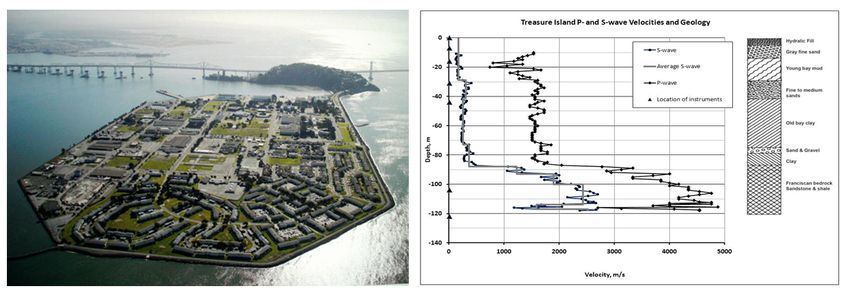
Page intentionally left blank
EXECUTIVE SUMMARY

For nuclear power plants licensed after January 10, 1997, Title 10 of the Code of Federal
Regulations (10 CFR) Part 50, “Domestic licensing of production and utilization facilities,” and
10 CFR 100.23, “Geologic and seismic siting criteria,” establish the seismic design basis.
Appendix S, “Earthquake Engineering Criteria for Nuclear Power Plants,” to 10 CFR Part 50
defines the safe-shutdown earthquake: “Safe-shutdown earthquake ground motion is the
vibratory ground motion for which certain structures, systems, and components must be
designed to remain functional.” The regulation in 10 CFR 100.23 requires that the applicant
determine the safe-shutdown earthquake and its uncertainty. A probabilistic seismic hazard
assessment (PSHA) is an acceptable method to capture uncertainty.

Traditionally, ground motion models and PSHAs are developed based on an ergodic
assumption, with a broad range of uncertainties. An ergodic process is a random process in
which the distribution of a random variable in space is the same as the distribution of that same
random variable at a single point when sampled as a function of time (Anderson and
Brune, 1999). An ergodic assumption is made when a PSHA treats that spatial uncertainty of
ground motions as an uncertainty over time at a single point. This usually results in overly
conservative values in hazard calculations. Recently, the practice has trended towards
nonergodic PSHAs, when additional information about the site of interest is available. It has
been previously shown that, with a sufficient number of earthquake recordings, the mean site
amplification functions (SAFs) can be well determined, but individual event ratios can be quite
variable. From this point of view, it is important to assess and quantify observed variabilities in
SAFs obtained from earthquake recordings.

This report assesses site-specific variability in empirical SAFs calculated using earthquake
recordings with a total of 13 datasets, including data from the six California strong motion
downhole arrays at Treasure Island, Turkey Flat, San Francisco Bay Bridge,
Crockett Carquinez Bridge, Corona Bridge, and Garner Valley and also three soil-rock pair
stations. The two- and three-dimensional effects, which include out-of-plane reflection/refraction,
focusing, scattering, and conversion of wave types, produce significant variability in empirical
SAFs from earthquake data recorded at a single station. This analysis demonstrates that log-
natural standard error σln(f) (sigma) in empirical SAFs calculated using downhole array data can
be approximated by a linear function with an average value of 0.221 (1.25 times) in the
frequency range of data processing. By using a constant in the frequency range of 0.1–10 hertz,
σln(f) can be well approximated and is slightly increasing at higher frequencies for rock-soil
pairs. Because of spatial variability, the rock-soil pairs sigma is higher than that of downhole
arrays with an average of 0.272 (1.31 times). Variability in empirical SAFs helps constrain
single-station, nonergodic sigma estimates.

    Keywords: Arrays Seismic Motion, Rock and Soil Motions, Site Amplification Variability
INTRODUCTION
For nuclear power plants licensed after January 10, 1997, Title 10 of the Code of Federal
Regulations (10 CFR) Part 50, “Domestic licensing of production and utilization facilities,” and
10 CFR 100.23, “Geologic and seismic siting criteria,” establish the seismic design basis.
Appendix S, “Earthquake Engineering Criteria for Nuclear Power Plants,” to 10 CFR Part 50
defines the safe-shutdown earthquake: “Safe-shutdown earthquake ground motion is the
vibratory ground motion for which certain structures, systems, and components must be
designed to remain functional.” The regulation in 10 CFR 100.23 requires that the applicant
determine the safe-shutdown earthquake and its uncertainty. A probabilistic seismic hazard
assessment (PSHA) is an acceptable method to capture uncertainty.

Traditionally, ground motion models and PSHAs are developed based on an ergodic
assumption, with a broad range of uncertainties. An ergodic process is a random process in
which the distribution of a random variable in space is the same as the distribution of that same
random variable at a single point when sampled as a function of time (Anderson and
Brune, 1999). An ergodic assumption is made when a PSHA treats that spatial uncertainty of
ground motions as an uncertainty over time at a single point. This usually results in overly
conservative values in hazard calculations. Recently, the practice has trended towards
nonergodic PSHAs, when additional information about the site of interest is available. It has
been previously shown that, with a sufficient number of earthquake recordings, the mean site
amplification functions (SAFs) can be well determined, but individual event ratios can be quite
variable (e.g., Field et al., 1992; Boore, 2004). From this point of view, it is important to assess
and quantify observed variabilities in SAFs obtained from earthquake recordings.

This report assesses site-specific variability in empirical SAFs observed using recorded
earthquake data from the six California strong motion downhole arrays at Treasure Island,
Turkey Flat, San Francisco Bay Bridge, Crockett Carquinez Bridge, Corona Bridge, and
Garner Valley and also three rock-soil pairs of stations. These downhole arrays have at least
one sensor in rock site condition. It also considers 13 alternative scenarios, giving the most
attention to the data from the Treasure Island and Turkey Flat arrays because these sites have
been studied extensively and have detailed geological and geotechnical information. Presented
uncertainties in SAFs are caused by randomness of earthquake locations and magnitudes and
can be considered to be aleatory.

      ANALYSIS OF THE TREASURE ISLAND DOWNHOLE ARRAY
                          RECORDS
Treasure Island (TI) is an artificial island in San Francisco Bay in California. Constructed in the
1930s for the 1939 Golden Gate International Exposition (Figure 1, left panel), the island was
created by fine-to-medium-grained sand dragged from San Francisco Bay and used as a fill
material. The fill material was deposited hydraulically by a clamshell dredge. Below the fill and
native sand is a layer of bay mud composed of silty clay with regions of sand and silt. The older
bay sediments of Pleistocene age are generally stiff to sandy, silty, or peaty clays that extend
down to Franciscan bedrock (Figure 1, right panel) (de Alba et al., 1994).

This report analyzes high-quality, low-amplitude earthquake data recorded at TI and Yerba
Buena Island (YBI) near San Francisco, CA. Most publications describe the YBI geology as rock
(e.g., Darragh and Shakal, 1991). TI is a manmade island situated between San Francisco and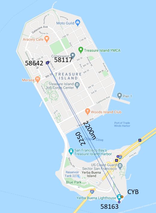
Oakland, CA, and attached to the natural YBI by a short causeway (Figure 1, left panel). Many
places on TI experienced liquefaction during the moment magnitude (M) 6.9 Loma Prieta
earthquake of 1989 (Ferritto, 1992). Following this earthquake, the California Geological Survey
(CGS), with support from the National Science Foundation, installed the TI array in 1992 to
study the response of a soft soil over rock geologic structure to earthquake motion (Darragh
et al., 1993; de Alba et al., 1994; Graizer, 2014). The TI downhole array had sensors located in
the bedrock (104- and 122-meter (m) depths), alluvium (31- and 44-m depths), and artificial fill
(7- and 16-m depths) and at the surface (shown with triangles in Figure 1, right panel). The
downhole instrument at 122-m depth was added in 1996. In September 2003, the original digital
12- and 16-bit instrumentation was replaced with modern 19-bit instruments (Graizer and
Shakal, 2004).

Figure 1 (right panel) shows the velocity and geology profiles at the TI array. Weathered
Franciscan shale and sandstone are encountered at 88 m beneath the site, with more
competent sandstone found at a depth of about 98 m (Darragh and Idriss, 1997). The
U.S. Geological Survey performed original downhole S-wave velocity measurements in the
104-m deep hole (Gibbs et al., 1992). More recent S-wave velocity averaging was performed
based on the P-S suspension logging measurements conducted in the deepest 122-m borehole
drilled in 1996 (Graizer and Shakal, 2004). S-wave velocities vary from ~134 meters per second
(m/s) in the gray fine sand layer to ~2,523 m/s in the deepest Franciscan bedrock (Figure 1,
right panel).

The authors downloaded 26 processed earthquake records from the Center for Engineering
Strong Motion Data (CESMD) https://strongmotioncenter.org/) recorded by the CGS Station
Treasure Island—Geotechnical Array. All recordings are low-amplitude ground motions with
maximum peak ground acceleration (PGA) at the surface of 0.038 g (Table 1). In contrast to
previous studies of TI recordings (Graizer, 2014), all except the local magnitude ML 5.0 1999
Bolinas earthquake were recorded by the array after September 2003 with the newly installed
modern 19-bit instruments that replaced the original 12- and 16-bit instrumentation (Graizer and
Shakal, 2004). Most of the older records were not used in order to avoid problems with low
signal-to-noise ratios especially affecting bedrock downhole recordings because of the lower
resolution of older equipment. First, the authors studied amplification of ground motions from the
deepest sensor in Franciscan bedrock at the depth of 122 m to the surface (Figure 1, right
panel) by comparing 5-percent damped response spectral accelerations of earthquake
recordings. At the second stage, the analysis examined amplification from bedrock recordings at
a depth of 104 m to the surface.

Figures 2 and 3 demonstrate examples of recorded accelerations and calculated displacements
at different depths representing the two different types of recordings: (1) relatively simple signals
dominated by S-waves (Figure 2) and (2) signals dominated by surface waves (Figure 3).

Figure 4 demonstrates response spectral ratios of motions at the surface relative to the bedrock
at 122-m depth. As is typical in earthquake engineering practice, individual earthquake SAFs at
each frequency are calculated as a ratio of geometric means of the two horizontal components
oriented at 90 and 360 degrees:

                                                  (     ,   ,      ,       )
                                    =                                                             (1)
                                                 (      ,   ,          ,   )
The main peak in the response spectral site amplification is observed at ~0.8 hertz (Hz), and the
second peak is at ~1.75 Hz (Figure 4). As shown by Haskell (1960), for a vertically incident
SH-wave on a plane layer having a shear wave velocity VS and a thickness h, mechanical
resonances occur at frequencies fn (quarter wavelength approximation):

                                           fn=(2n+1)×VS /4h                                     (2)

The lowest frequency (first mode) can be associated with the alluvium-bedrock interface at the
88-m depth characterized by the S-wave velocity increase from 386 to 1,230 m/s (Figure 1, right
panel). Using average S-wave velocity of VS ~267 m/s in the upper layer of thickness h = 88 m
results in the resonance frequency of 0.76 Hz, which is close to the average empirical value of
0.8 Hz. The second peak in SAF at 1.75 Hz can be associated with the bay mud-alluvium
interface at the depth of 28.8 m, characterized by a significant S-wave velocity increase from
176 to 317 m/s.

SAFs shown in Figure 4 (upper panel) demonstrate significant variations in amplitudes of the
first peak at ~0.8 Hz from a factor of ~4 to ~13 for individual events. These SAFs can be split
into the two different groups depending on the amplitudes of the first ~0.8-Hz peak: the lower
amplification group (LAG) events (maximum peak averages ~4.9) (Figure 4, middle panel) and
the higher amplification group (HAG) events (maximum peak averages ~9.0) (Figure 4, lower
panel). The first group (LAG) includes 14 events, and the second one (HAG) includes 12 events
(Table 1). Events that produce lower amplitude spectral ratios are mostly close-by earthquakes
with dominant direct S-waves and relatively low-amplitude surface waves (Figure 2).
Earthquakes producing relatively higher amplitude response spectral ratios are more distant
earthquakes with larger amplitude surface waves compared to S-wave amplitudes (Figure 3).

Figure 5 demonstrates mean ±1 standard deviation response SAFs for all 26 surface/122-m
depth records and also for the LAG and HAG. As expected, the group that includes all events
demonstrates higher log-natural sigma σln(f) than that of the low SAF events. In all cases,
average sigmas are almost flat with only slight change at frequencies higher than 30 Hz.

At the second stage, the authors calculated SAFs for 11 surface/104-m depth available records.
Unfortunately, after 2007, the three channels in the 104-m deep downhole died and did not
record earthquakes. SAFs shown in Figure 6 demonstrate first and second peaks at the same
frequencies of 0.8 and 1.8 Hz and also significant variations in amplitudes of the first peak in
individual events. This group of recordings demonstrates practically flat log-natural sigma σln(f),
very similar to that of 122-m downhole up to the frequency of 30 Hz. In the frequency range of
data processing of 0.3–40 Hz, average sigma is slightly higher for the surface/104-m case
(0.202 versus 0.189).

      TREASURE ISLAND AND YERBA BUENA ISLANDS GROUND
                          MOTIONS
In the next series of tests, the analysis compares YBI surface recordings at two nearby stations
with the response of the TI array surface data (downhole horizontal Channels 1 and 3 of CGS
Station 58642). The stations are (1) YBI CGS Station 58163 and (2) YBI CYB USGS-NCSN
station (Table 2).
TI is connected by a small isthmus to YBI with the distance between those sites of 2.20 and
2.25 kilometers (km) (Figure 7). Most publications describe the geology of YBI as rock
(Franciscan formation with a mix of sandstone, limestone metamorphic, and other rocks)
(Darragh and Shakal, 1991; Darragh and Idriss, 1997; Baise et al., 2003), while the CESMD
Web site (https://strongmotioncenter.org/) estimates VS30 at 660 m/s and considers it to be
Class C. Liquefaction occurred at TI during the 1989 M 6.9 Loma Prieta earthquake (Ferritto,
1992; de Alba et al., 1994).
The authors downloaded YBI data from the CESMD for seven earthquakes that were also
recorded by the TI array surface channels. Figure 8 (upper panel) demonstrates horizontal
component response spectral ratios between the TI surface and YBI. The data were split into
two groups: five records from earthquakes with M≤4.5 and all seven events including the M 6.9
Loma Prieta and the South Napa M 6.0 earthquakes. Because of liquefaction at TI, the
Loma Prieta record is affected by the nonlinearity with a shift of peak SAF toward low
frequencies. As expected, σln(f) is lower for the first group of smaller events not affected by
nonlinearity. The two main peaks in site amplifications are at the frequencies of ~0.8 and
1.8 Hz, demonstrating similarity to those of the TI downhole array shown in Figures 4 through 6.
A number of previous studies (e.g., Darragh and Shakal, 1991) have used rock ground motions
at YBI as a reference site to estimate the site response at TI applying a one-dimensional
equivalent linear approach. Baise et al. (2003) demonstrated that a two-dimensional basin
structure is needed to analyze TI site response. A comparison of SAFs from the YBI and TI
bedrock 122-m depth recordings in Figure 8 (lower panel) demonstrates an average
amplification of 3.5 times at 10–20 Hz at the YBI relative to TI bedrock, while at frequencies
higher than 30 Hz, the difference is about 2.35 (close to the theoretical one of ~2.0) between the
media motion relative to the outcrop. These comparisons show that the YBI site is not an ideal
rock site input for the TI surface recordings.
TURKEY FLAT ARRAY RECORDINGS
The CGS established the Turkey Flat Site Effects International Test Area in 1987, in a shallow
valley at Turkey Flat, located 8 km southeast of the town of Parkfield and about 5 km east of the
San Andreas Fault in central California. The array was intended to provide data with which to
investigate the accuracy and consistency of current methods for estimating the effects of site
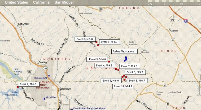
conditions on ground surface motions (Real and Tucker, 1988). Figure 9 shows the location of
the Turkey Flat strong motion array and epicenters of the eight earthquakes used in the
prediction exercise provided by the CGS and two additional events (9 and 10), shown in
Table 3, downloaded from the CESMD at https://strongmotioncenter.org/.
The Turkey Flat array is located in a northwest-trending valley within the central California
Coastal Range. The valley is filled with a relatively thin layer of stiff alluvial sediments with
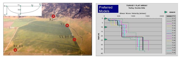
basement rock outcrops at the south and north ends of the valley (Figure 10, left panel). The
valley is about 6.5 km long and 1.6 km wide and is aligned with the southwest plunging Parkfield
syncline (Real and Tucker, 1988). Turkey Flat was chosen as a test area to begin with a
geologically simple site where a moderate event producing strong motion is expected before
moving to more complicated sites.
The Turkey Flat array includes four recording sites: Rock South or Turkey Flat #1 (TF#1) (R1 in
Figure 10), Valley Center or Turkey Flat #2 (TF#2) (V1), Valley North or Turkey Flat #3 (TF#3)(V2), and Rock North or Turkey Flat #4 (TF#4) (R2). Surface instruments were installed at each of these sites, and downhole instruments were installed at the Rock South (R1) and Valley Center (V1) sites. Downhole instrument D1 was located at a depth of approximately 24 m at the Rock South site, and downhole instruments D2 and D3 were located at depths of 10 m and 23.5 m, respectively, at the Valley Center. Valley Center instrument D3 (23.5-m depth) was located about 1 m below the soil/rock boundary. Each instrument location included a three- component force-balance accelerometer and a velocity transducer with 12-bit solid-state digital recording. Unfortunately, the downhole E-W oriented sensor at TF#1 did not work. For reference, the distance from V1 to V2 is about 510 m, from V1 to R1 about 850 m, and from V2 to R2 550 m. The distance between R1 and R2 is about 1,600 m (Figure 10, left panel). In 1987–1988, multiple investigation teams, both domestic and abroad, carried out a comprehensive program of site characterization. The teams conducted a broad range of field and laboratory geophysical and geotechnical tests. Eight boreholes were drilled through valley sediments into the underlying basement rocks, in which in situ testing was performed and rock and sediment samples were acquired for laboratory analysis. Shear-wave velocity (Figure 10, right panel) was measured in boreholes at the two vertical arrays using downhole, crosshole, and suspension logging methods performed by numerous groups, including LeRoy Crandall and Associates, Hardin Lawson Associates, QEST Consultants, OYO Corporation, Kajima Corporation, the California Division of Mines and Geology (renamed California Geological Survey in 2006), and Woodward–Clyde Consultants (Real et al., 2008; Haddadi et al., 2008; Real and Tucker, 1988). All records used for this analysis except for the M 6.0 Parkfield 2004 earthquake are low-amplitude ground motions indicative of mostly linear site amplifications (Table 3). The Parkfield earthquake was recorded at an epicentral distance of less than 10 km with PGA up to 0.3 g at the TF#2 (Valley Center) site. Usually, amplitudes higher than 0.2–0.3 g are considered to be the level where nonlinearity effects start. According to the results compiled by Kramer (2009), the site responded essentially linearly in the 2004 Parkfield event. One of the purposes of establishing the Turkey Flat array and an international test area was to perform a blind test experiment similar to that done in typical construction projects. In the first phase of the blind test experiment, participants were provided with all available subsurface data and the recorded R1 rock motions and asked to predict the response of the Valley Center V1 soil motion 850 m apart. In the second phase, which did not begin until all first-phase predictions had been received, participants were provided with the D3 motions and asked to predict the D2 and V1 motions. A number of papers describe the results of the experiment (e.g., Kwok et al., 2008; Kramer, 2009). All the strong motion earthquake records except for Parkfield main shock were processed in the frequency range of 0.3–40 Hz. The M 6.0 Parkfield record was processed in the frequency range of 0.125–40 Hz. This report considers empirical SAFs. Site amplifications were calculated for the following four cases: (1) Valley Center downhole TF#2 bedrock (23.5-m depth) to surface (Figure 11) (2) Rock South (TF#1) to Valley Center (TF#2) surface motions (Figure 12)
(3)    Rock North (TF#4) to Valley North (TF#3) (Figure 13)
(4)    Combined rock (Rock South + Rock North) to combined soil (Valley Center + Valley
       North) (Figure 14)

Empirical SAFs demonstrate significant variabilities for different events (Figures 11 through 14),
with the average log-natural sigma varying in the range from σln=0.262 to σln=0.340 with the
highest variability observed in the Rock South–Valley Center outcrops (Figure 12), and the
lowest for Rock North–Valley North outcrops (Table 4 and Figure 13).

The transfer function V1 (TF#2 surface) – R1 (TF#1 surface) has the highest natural variability
of σln=0.340 between analyzed pairs. Natural variability in SAFs between TF#2 downhole
bedrock (23.5 m deep) and surface motion is relatively high (σln=0.288), considering the
relatively simple Turkey Flat geologic structure. Tsai et al. (2017) suggested that the
two-dimensional effect influenced the response at sites located near the edge of the basin and
makes SAFs dependent on wave propagation paths.

       ADDITIONAL DOWNHOLE DATA AND SUMMARY RESULTS
This study also included two sets of 16 earthquakes recorded at the Garner Valley downhole
array (GVDA) at the surface and at the depths of 50 m (VS=580 m/s) and 150 m (VS=3,000 m/s).
GVDA records were downloaded from http://nees.ucsb.edu/data-portal. Appendix A (Figure A-1)
shows the GVDA sensor locations and P- and S-wave velocity profiles. GVDA σln demonstrates
the same behavior as others outlined above: it is almost flat from 0.3 to 40 Hz (Figure 15).

Additionally, the authors analyzed earthquake recordings from the three CGS instrumented
strong-motion downhole arrays: San Francisco Bay Bridge with the deepest sensor at 39.9 m
and corresponding VS ~2,000 m/s (10 earthquakes), Crockett Carquinez Bridge #2 with the
deepest sensor at 125 m and VS >1,000 m/s (8 earthquakes), and Corona–I15/Hwy 91
(11 earthquakes) with the deepest sensor at 41.8 m and VS ~2,000–3,000 m/s. Data were
downloaded from the CESMD at https://strongmotioncenter.org/. Appendix A (Figures A-2, A-3,
and A-4) shows schematics of downhole locations and P- and S-wave velocity profiles.

Figure 15 and Table 4 show a compilation of all data from downhole arrays and an average
sigma. In almost all cases, log-natural sigma can be approximated by linear dependence with a
low slope. Average logarithmic sigma is practically flat in the frequency range 0.1 to 100 Hz.

All this can be considered as aleatory variability and also as the lowest end of nonergodic
site-specific sigma. In average log-natural sigma, σln(f) from downhole array data varies:

                   σln(f)= 0.0000005×f+0.2351                                                   (3)

In the data processing frequency range of 0.3–40 Hz, standard error σln(f) in empirical site
amplification has an average value of 0.221 (1.247 times the mean value of SAF).
This variability in site amplification is due to variations in site-to-source azimuths, wave
propagation paths and wave types, magnitudes of earthquakes, and nonlinearity effects
modifying amplitudes of ground motions at the site. All data considered in this paper except for
the moment magnitude MW 6.9 Loma Prieta 1989 and the MW 6.0 Parkfield 2004 earthquakes
are low-amplitude recordings with no nonlinearity effects.
For soil-rock pairs, the average sigma σln(f) can be approximated as follows:
σln(f)= 0.0017×f+0.2525 (4)
As expected, because of spatial variability the soil-rock pair sigma is higher than that of the
downhole arrays with an average of 0.272 (1.31 times the mean value of SAF) in the 0.3–40 Hz
frequency range (Figure 16). The increase of sigma at high frequencies can be explained by
(1) increased randomness at frequencies ≥10 Hz, (2) variation of incident wave angles,
(3) variations in media resulting from different paths, and (4) increase of instrumental noise at
higher frequencies.
The results of this study agree with Boore’s (2004) observation that variability in ground motions
is large, making it difficult to accurately predict site- and earthquake-specific response, and with
its recommendation to concentrate on predicting mean amplifications for many events.
CONCLUSIONS
This analysis assessed site-specific variability in empirical SAFs calculated using earthquake
recordings of a total of 13 datasets, including data from the six California strong motion
downhole arrays at Treasure Island, Turkey Flat, San Francisco Bay Bridge,
Crockett Carquinez Bridge, Corona Bridge, and Garner Valley and also three soil-rock pairs of
stations.
In the frequency range of 0.1–100 Hz, log-natural standard error σln(f) in empirical downhole site
amplification can be approximated by a linear function with an average value of 0.221
(1.25 times the mean value of SAF). For frequencies ≤10 Hz σln(f), function is practically flat and
starts increasing at higher frequencies for soil-rock pairs. The lowest sigma corresponds to the
downhole amplification associated with the vertically propagating S-waves, while the highest
sigma is associated with a rock-soil TF#1 and TF#2 pair where rock station is located near the
edge of the two-dimensional basin. As expected, because of spatial variability in soil, the rock
pairs sigmas on average are higher (0.272) than those of downhole arrays (average of 0.221)
(Figure 16).
The two- and three-dimensional effects, which include lateral refraction, focusing, scattering,
and conversion of wave types, produce significant variability in empirical SAFs from earthquake
data recorded at a single station and help constrain single-station, nonergodic sigma estimates.
The results also give insights into the accuracy that can be achieved in site response
predictions. Standard error estimates based on downhole array data represent aleatory
variability and can also be considered as the lowest end of nonergodic site-specific sigma.DATA AND RESOURCES
GVDA data and information were downloaded from http://nees.ucsb.edu/data-portal. All other
earthquake records and downhole information were downloaded from the CESMD at
https://strongmotioncenter.org/.
ACKNOWLEDGMENTS
We appreciate help from Hamid Haddadi and David Branum in providing additional strong
motion data and supporting information about California Geological Survey stations. We thank
J.P. Stewart for sharing Turkey Flat geotechnical profiles data.
REFERENCES
Anderson, J., and J. Brune (1999). “Probabilistic seismic hazard assessment without the ergodic
assumption,” Seism. Res. Lett. 70, 19–28.
Baise L.G, S.D. Glaser, and D. Dreger (2003). “Site response at Treasure and Yerba Buena
Islands, California,” Journ. Geotechnical and Geoenvironmental Engineering. 129 (5):415–426.
Boore, D.M. (2004). “Can site response be predicted?” Journ. Earthquake Engineering. 8,
Special Issue 1. 1–41.
Darragh, R.B., and I.M. Idriss (1997). “A Tale of Two Sites: Gilroy #2 and Treasure Island Site
Response Using an Equivalent Linear Technique,” Earthquake Engineering Research Institute,
Oakland, CA.
Darragh, R.B., and A.F. Shakal (1991). ‘‘The site response of two rock and soil station pairs to
strong and weak ground motion,’’ Bull. Seismol. Soc. Am., 81, 1885–1899. Darragh, R., M.
Huang and A. Shakal (1993). "Processed CSMIP strong-motion data from the Treasure Island
geotechnical array from the Gilroy area earthquake of January 16, 1993." Calif. Div. Mines and
Geology, OSMS 93-09, 37 p.
de Alba, P., J. Benoit, D.G. Pass, J.L. Carter, T.L. Youd, and A.F. Shakal (1994). “Deep
instrumentation array at Treasure Island Naval Station,” U.S. Geol. Surv. Prof. Pap. 1551-A,
155–168.
Ferritto, J.M. (1992). “Ground motion amplification and seismic liquefaction: A study of Treasure
Island and the Loma Prieta earthquake,” Naval Civil Engineering Laboratory (NCEL) Technical
Note 92-21874, Port Hueneme, CA.
Field, E.H., K.H. Jacob, and S.E. Hough (1992). “Earthquake site response estimation: A
weak-motion case study,” Bull. Seism. Soc. Am. 82, 2283–2307.
Gibbs, J.F., T.E. Fumal, D.M. Boore, and W.B. Joyner (1992). “Seismic velocities and geological
logs from borehole measurements at seven strong-motion stations that recorded the
Loma Prieta earthquake,” U.S. Geological Survey Open-File Report 92-287, Menlo Park, CA.Graizer, V., and A.F. Shakal (2004). “Analysis of CSMIP strong-motion geotechnical array recordings,” in P. de Alba, R.L. Nigbor, J.H. Steidl, and J.C. Stepp, editors, In Proceedings: International Workshop for Site Selection, Installation, and Operation of Geotechnical Strong- Motion Arrays, Richmond, CA, 2004. Consortium of Organizations for Strong Motion Observation Systems (COSMOS). Graizer, V. (2014). “Comment on ‘Comparison of time series and random-vibration theory site-response methods’ by Albert R. Kottke and Ellen M. Rathje,” Bull. Seismol. Soc. Am., 104, 540–546. Haddadi, H., A.F. Shakal, and C.R. Real (2008). “The Turkey Flat Blind Prediction Experiment for the September 28, 2004 Parkfield Earthquake: Comparison with Other Turkey Flat Recordings,” Geotechnical Earthquake Engineering and Soil Dynamics IV Congress 2008, pp. 1–10. Haskell, N. (1960). “Crustal reflection of plane SH waves,” J. Geophys. Res. 65, 4147–4450. Kramer, S.L. (2009). “Analysis of Turkey Flat ground motion prediction experiment—Lessons learned and implication for practice,” Proc. SMIP09 Seminar on Utilization of Strong-Motion Data, Oakland, CA, pp.1–22. Kwok, A.O.L., J.P. Stewart, and Y.M.A. Hashash (2008). “Nonlinear ground-response analysis of Turkey flat shallow stiff-soil site to strong ground motion,” Bull. Seismol. Soc. Am. 98, 331– 343. Real, C.R. and B.E. Tucker (1988). “Ground Motion Site Effects Test Area Near Parkfield, California,” Proceedings Ninth World Conference on Earthquake Engineering, Tokyo, Japan VIII, pp. 187–191. Real, C.R., A.F. Shakal, and B.E. Tucker (2006). “Turkey Flat, U.S.A. site effects test area: Anatomy of a blind ground-motion prediction test,” Proceedings, 3rd International Symposium Effects of Surface Geology on Seismic Motion, 29 August–1 September 2006, Grenoble, France, Paper KN 3, pp. 1–19. Real, C., A. Shakal, and B. Tucker (2008). “The Turkey Flat Blind Prediction Experiment for the September 28, 2004 Earthquake: General Overview and Models Tested,” Geotechnical Earthquake Engineering and Soil Dynamics IV Congress 2008, pp. 1–10. Tsai, C.-C., W.-S. Chang, and J.-S. Chiou (2017). “Enhancing Prediction of Ground Response at the Turkey Flat Geotechnical Array,” Bull. Seismol. Soc. Am. 107, 2043–2054. U.S. Code of Federal Regulations, “Reactor Site Criteria,” Part 100, Chapter I, Title 10, “Energy.” U.S. Code of Federal Regulations, “Domestic Licensing of Production and Utilization Facilities Part 50, Chapter I, Title 10, “Energy”.
Figure 1. View of TI and YBI (left panel) and P- and S-wave velocities and soil profile at TI
          array (right panel). Triangles show locations of seismic instruments.

Figure 2. Shear waves dominated record of the ML 3.4 earthquake with the epicenter at
          Berkeley, CA, at a distance of 12.5 km (Table 1): acceleration (left panel) and
          displacement (right panel).
Figure 3. Surface waves dominated record of the MW 4.2 earthquake with the epicenter at
Piedmont, CA, at a distance of 16.5 km (Table 1): acceleration (left panel) and
displacement (right panel).Figure 4. Response SAFs from bedrock at 122-m depth to the surface at the TI array:
records from all 26 events (upper panel), records from 14 LAG events (middle
panel), and records from 12 HAG events (lower panel).Rat_1
Treasure Island Spectral Amplification Functions Surf/122 m Rat_2
Rat_3
Rat_1
Rat_2
10 Rat_3
Response Spectral Amplification and Sigma
Rat_4
Rat_5
Rat_6
Rat_7
Rat_8
Rat_9
Rat_10
Rat_11
Rat_12
1 Rat_13
Rat_14
Rat_15
y = -0.0005x + 0.2338 High Rat_16
Rat_17
Rat_18
Rat_19
Rat_20
Rat_21
0.1 Rat_22
Rat_23
y = -0.0009x + 0.2218 All y = -4E-05x + 0.1415 Low Rat_24
Rat_25
Rat_26
Mean_all
STD_All
Mean+1std
Mean-1std
Mean_low
0.01 STD_Low
Frequency, Hz MeanL+1std
0.1 1 10 100 MeanL-1std
Figure 5. Response spectral SAFs and natural logarithmic standard deviations of SAFs
for the TI downhole array surface/122-m depth.
Treasure Island Spectral Amplification Functions Surf/104 m
Rat_1
10
Response Spectral Amplification and Sigma
Rat_2
Rat_3
Rat_4
Rat_5
Rat_6
1 Rat_7
Rat_8
y = -0.0002x + 0.2242 Surf/104 m Rat_9
Rat_10
Rat_11
104_Mean_SAF
0.1 y = -0.0009x + 0.2218 Surf/122 m
104_Mean-1std
104_Mean+1std
104_STD
122_STD
Linear (104_STD)
0.01
Linear (122_STD)
0.1 1 10 100
Frequency, Hz
Figure 6. Response SAFs and natural logarithmic standard deviations of SAFs for the TI
downhole array surface/104-m depth.Figure 7. Map of TI and YBI stations. 58117 is the old TI Fire Station, and 58163 is the
YBI Station. Those two stations recorded the 1989 M 6.9 Loma Prieta
earthquake.Treasure - Yerba Island SAF Berkeley_2011_NCCYB
10 Berkeley_2011_CSMIP
Response Spectral Amplification and Sigma
ElCerrito_2012_CSMIP
Berkeley_2018_CSMIP
Berkeley_2018_NCCYB
Mean_low
Mean+1std
1 Mean-1std
LomaPrieta_1989
y = 0.0025x + 0.2735 all Napa_2014_NCCYB
Log_std_low
Mean_all
Mean+1std
y = 0.0014x + 0.1792 low Mean-1std
0.1
Log_std_all
Linear (Log_std_low)
Linear (Log_std_all)
0.01
0.1 1 Frequency, Hz 10 100
10
Ratio Yerba Buena to TI 122 m depth
Response Spectral Amplification and Sigma
1
y = 0.0037x + 0.1577
Berkeley_2011_NCCYB
0.1 Berkeley_2011_CSMIP
ElCerrito_2012_CSMIP
Napa_2014_NCCYB
Geomean
Log_Std
Mean+1sigma
Mean-1sigma
Linear (Log_Std)
0.01
0.1 1 Frequency, Hz 10 100
Figure 8. Response spectral SAFs and natural logarithmic standard deviations of SAFs
for the TI surface to YBI (upper panel), and comparison of SAFs from the YBI to
TI bedrock 122-m depth recordings (lower panel).Figure 9. Map of earthquakes and Turkey Flat strong motion stations (modified from
Haddadi et al., 2008).
Figure 10. Oblique aerial view of Turkey Flat strong-motion array (Real et al., 2008) (left
panel) and S-wave velocity profiles at mid-valley site (V1-D3 array) from
Real et al., 2006 (right panel).Turkey Flat #2 Surface/Downhole 23.5 m SAF
10
Response Spectral Amplification and Sigma
Ratio_1
1 Ratio_2
Ratio_3
Ratio_4
Ratio_5
Ratio_6
Ratio_7
Ratio_8
Ratio_9
y = 0.0034x + 0.2489 Ratio_10
0.1 Mean_Ratio
Mean+1std
Mean-1std
Log_Stdev
Linear (Log_Stdev)
0.01
0.1 1 Frequency, Hz 10 100
Figure 11. Response spectral SAFs and natural logarithmic standard deviations of SAFs
for the Turkey Flat downhole array TF#2.
10
Turkey Flat TF#2 Surface (soil) to TF#1 Surface (rock)
Response Spectral Amplification and Sigma
Ratio_Ev_1
Ratio_Ev_2
Ratio_Ev_3
1 Ratio_Ev_4
Ratio_Ev_5
Ratio_Ev_6
Ratio_Ev_7
Ratio_Ev_8
Ratio_Ev_9
Ratio_Ev_10
y = 0.0015x + 0.3272
Log_N_TF1_TF2
0.1
Mean
Mean+1sd
Mean-1sd
Linear (Log_N_TF1_TF2)
0.01
0.1 1 Frequency, Hz 10 100
Figure 12. Response spectral SAFs and natural logarithmic standard deviations of SAFs
for the Turkey Flat downhole array TF#2 surface to TF#1 surface.Turkey Flat TF#3 (soil) to TF#4 (rock) SAF
10
Response Spectral Amplification and Sigma
1
Ratio_1
Ratio_2
Ratio_3
Ratio_4
Ratio_6
Ratio_7
0.1 y = 0.0024x + 0.2287
Ratio_8
Mean
Log_N_TF3_TF4
Mean+1std
Mean-1std
Linear (Log_N_TF3_TF4)
0.01
0.1 1 Frequency, Hz 10 100
Figure 13. Response spectral SAFs and natural logarithmic standard deviations of SAFs
for TF#3 (soil) to TF#4 (rock).
Turkey Flat Average Soil to Average Rock SAFs
10
Response Spectral Amplification and Sigma
Ratio_1
Ratio_2
Ratio_3
Ratio_4
1 Ratio_5
Ratio_6
Ratio_7
Ratio_8
Ratio_9
y = 0.0016x + 0.275 Ratio_10
Mean
0.1 Mean+1std
Mean-1std
Log-N_all
Linear (Log-N_all)
0.01
0.1 1 10 100
Frequency, Hz
Figure 14. Response spectral SAFs and natural logarithmic standard deviations of SAFs
for the Turkey Flat average soil/rock.1
TI_122m
Downhole Arrays Sigma
TI_104m
Corona
TF#2
SanFrancisco
Ln Sigma
Carquinez_2
0.1
GV_50
y = -7E-05x + 0.2351
GV_150
Av Sigma
Av+1std
Av-1std
Linear (Av
Sigma)
0.01
0.1 1 Frequency, Hz 10 100
Figure 15. Frequency dependence of sigma σln of the SAFs.
1
Soil - Rock Sigma
y = 0.0017x + 0.2525 soil-rock
Ln Sigma
Yerba_TI
TF1_TF2
0.1 y = -7E-05x + 0.2351 downholes
TF3_TF4
TF_Soil_Rock
Soil/Rock
Sigma Downholes
Linear (Soil/Rock)
Linear (Sigma Downholes)
0.01
0.1 1 Frequency, Hz 10 100
Figure 16. Soil-rock station pairs sigma compared to downhole arrays sigma.APPENDIX A
ADDITIONAL DOWNHOLE ARRAYS SCHEMATIC SENSOR LOCATIONS AND P- AND S-
WAVES VELOCITY PROFILES
Figure A-1. Garner Valley downhole array (GVDA) and P- and S-wave velocity profiles.
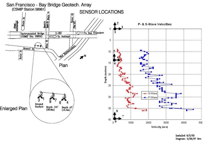
Downloaded from http://nees.ucsb.edu/facilities/GVDA.Figure A-2. San Francisco Bay Bridge Geotech Array (58961). Sensors: Surface,14.3,
39.9 meters (m). Downloaded from the Center for Engineering Strong Motion
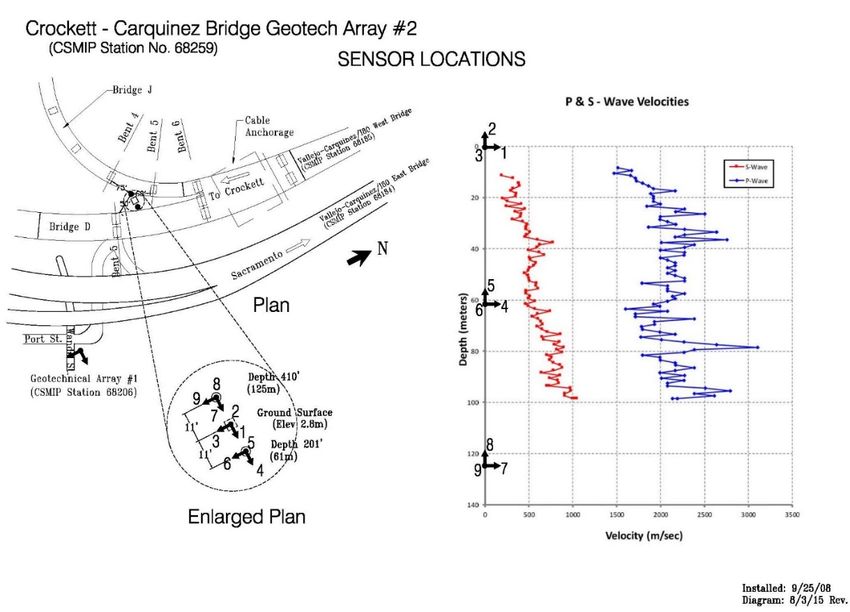
Data (CESMD) at https://strongmotioncenter.org/.Figure A-3. Crockett Carquinez Bridge Geotech Array #2 (68259). Sensors: Surface, 61,
125 m. Downloaded from the CESMD at https://strongmotioncenter.org/.Figure A-4. Corona–I15/Hwy 91 Geotech Array (13186). Sensors: Surface, 7.9, 21.6,
41.8 m. Downloaded from the CESMD at https://strongmotioncenter.org/.Table 1. Earthquakes recorded at the Treasure Island geotechnical array at the surface
and at 122-m depth
Depth, Epicenter Surface
Earthquake Name Date Time Magnitude km Dist., km PGA
S-waves dominated lower amplification group
Bolinas 1999-08-17 18:06:18 PDT 5.0 ML 6.9 29.0 0.018
Piedmont 2005-05-08 3:35:55 PDT 3.3 MW 5.0 13.1 0.003
Piedmont 2005-09-24 4:25:16 PDT 3.3 MW 5.4 13.5 0.002
Berkeley 2006-12-22 22:49:57 PST 3.6 ML 9.2 11.9 0.029
Berkeley 2006-12-23 09:21:15 PST 3.4 ML 9.3 11.6 0.015
Berkeley 2007-02-23 15:46:15 PST 3.4 ML 10.9 12.5 0.019
Alamo 2008-09-05 21:00:15 PDT 4.0 MW 16.2 33.6 0.025
Berkeley 2009-05-13 15:34:05 PDT 3.1 MW 10.8 13.2 0.004
San Francisco 2010-06-28 07:47:04 PDT 3.3 MW 7.7 18.6 0.003
Morgan Hill 2011-01-07 16:10:16 PST 4.1 ML 7.1 86.5 0.005
Berkeley 2011-10-20 14:41:04 PDT 4.0 MW 8.0 11.7 0.023
Berkeley 2011-10-20 20:16:05 PDT 3.8 MW 9.6 11.8 0.038
Berkeley 2011-10-27 05:36:44 PDT 3.6 ML 9.7 12.1 0.013
El Cerrito 2012-03-05 05:33:19 PST 4.0 ML 9.2 13.1 0.019
Surface waves dominated higher amplification group
11:15:56 AM
San Simeon 2003-12-22 PST 6.5 MW 4.7 261.0 0.004
Orinda 2006-03-01 11:34:52 PST 3.4 MW 8.3 14.9 0.006
Glen Ellen 2006-08-02 20:08:12 PDT 4.4 ML 9.1 52.1 0.014
Lafayette 2007-03-01 20:40:00 PST 4.2 ML 16.6 25.7 0.014
Berkeley 2011-07-16 03:31:26 PDT 3.3 MW 6.0 11.0 0.004
Piedmont 2007-07-20 04:42:22 PDT 4.2 MW 5.8 16.5 0.018
San Leandro 2011-08-23 23:36:54 PDT 3.6 ML 8.1 21.8 0.007
Alum Rock 2007-10-30 20:04:54 PDT 5.4 MW 9.2 68.5 0.012
Moraga 2008-06-06 02:02:53 PDT 3.5 MW 7.6 26.3 0.003
El Cerrito 2009-06-06 15:30:56 PDT 3.3 MW 5.6 12.0 0.003
South Napa 2014-08-24 03:20:44 PDT 6.0 MW 11.3 44.1 0.017
Pleasant Hill 2019-10-14 22:33:42 PDT 4.5 MW 14.0 30.5 0.011Table 2. Earthquakes recorded at Yerba Buena and surface channels of Treasure Island
Epicenter Surface Epicenter
Earthquake Depth, Dist., km PGA Dist., km PGA
Name Date Time Magnitude km Treasure Island Yerba Buena
Loma Prieta 1989-10-17 17:04:00 PDT 6.9 MW 18.0 97.7 0.160 95.4 0.060
Berkeley 2011-10-20 14:41:04 PDT 4.0 MW 8.0 11.7 0.023 11.7 0.021
Berkeley 2011-10-20 20:16:05 PDT 3.8 MW 9.6 11.8 0.038 11.8 0.039
El Cerrito 2012-03-05 05:33:19 PST 4.0 ML 9.2 13.1 0.019 14.5 0.015
South Napa 2014-08-24 03:20:44 PDT 6.0 MW 11.3 44.1 0.017 45.9 0.005
Berkeley 2018-01-04 02:39:37 PDT 4.4 MW 12.3 10.8 0.064 10.7 0.042
Pleasant Hill 2019-10-14 22:33:42 PDT 4.5 MW 14.0 30.5 0.011 30.5 0.005
Table 3. Events producing moderate to strong motions at Turkey Flat array (updated after
Haddadi et al., 2008)
Event Event Epicenter Distance from Epicenter to: PGA @ Surface
No. Name Date Time Mag Lat Lon TF#1 TF#2 TF#3 TF#4 TF#1 TF#2 TF#3 TF#4
1 Parkfield 4/3/1993 21:21:24 PST 4.2 35.942 120.493 14.1 14.5 14.3 13.9 0.026 0.033 0.081 0.047
2 San Simeon 12/22/2003 11:15:56 PST 6.5 35.710 121.100 69.6 70.4 70.6 70.6 0.035 0.036 0.031 0.023
Parkfield
3 (Mainshock) 9/28/2004 10:15:24 PDT 6.0 35.810 120.370 7.6 8.2 8.6 9.2 0.245 0.300 0.260 0.110
4 Aftershock 9/28/2004 10:19:24 PDT 4.2 35.844 120.402 5.5 6.3 6.6 7.0 0.052 0.170 0.072 0.034
5 Aftershock 9/28/2004 10:24:15 PDT 4.7 35.810 120.350 7.6 8.0 8.4 9.1 0.046 0.074 0.053 0.013
6 Aftershock 9/28/2004 10:33:56 PDT 3.7 35.815 120.363 7.0 7.5 8.0 8.6 0.016 0.026 0.026 0.006
7 Aftershock 9/28/2004 12:31:27 PDT 4.0 35.840 120.390 5.1 5.9 6.3 6.7 0.012 0.049 0.024 0.008
8 Aftershock 9/29/2004 10:10:04 PDT 5.0 35.954 120.502 15.5 15.9 15.7 15.2 0.016 0.042 0.037 0.030
9 Parkfield 5/22/2007 04:34:12 PDT 4.0 35.860 120.414 5.4 6.3 NR* NR 0.035 0.054 NR NR
10 Cholame 12/17/2019 10:29:21 PST 4.3 35.806 120.356 7.9 8.5 NR NR 0.051 0.047 NR NRTable 4. Average logarithmic standard deviation
Average in range of 0.3–40 Hz
Site Log_Nat_Sigma σln Ratio
Treasure Island 122 m 0.189 1.208
Treasure Island 104 m 0.202 1.224
Corona Bridge 0.282 1.326
TF#2 0.287 1.332
San Francisco Bay Bridge 0.211 1.235
Crockett Carquinez_2 0.216 1.241
Garner Valley 50 m 0.163 1.177
Garner Valley 150 m 0.218 1.243
Av Sigma 0.221 1.247
Yerba_TI 0.203 1.225
TF1_TF2 0.341 1.407
TF3_TF4 0.263 1.301
TF_Soil_Rock 0.282 1.326
Av Sigma 0.272 1.313You can also read