Atmospheric Electric Field-Mill Sensor Field Campaign Report - DOE/SC-ARM-21-013
←
→
Page content transcription
If your browser does not render page correctly, please read the page content below
DOE/SC-ARM-21-013

Atmospheric Electric Field-Mill Sensor Field
Campaign Report

HG Silva     FM Lopes

July 2021
DISCLAIMER

This report was prepared as an account of work sponsored by the U.S.
Government. Neither the United States nor any agency thereof, nor any of
their employees, makes any warranty, express or implied, or assumes any
legal liability or responsibility for the accuracy, completeness, or
usefulness of any information, apparatus, product, or process disclosed, or
represents that its use would not infringe privately owned rights. Reference
herein to any specific commercial product, process, or service by trade
name, trademark, manufacturer, or otherwise, does not necessarily
constitute or imply its endorsement, recommendation, or favoring by the
U.S. Government or any agency thereof. The views and opinions of
authors expressed herein do not necessarily state or reflect those of the
U.S. Government or any agency thereof.
DOE/SC-ARM-21-013

Atmospheric Electric Field-Mill Sensor Field
Campaign Report

HG Silva, University of Évora
FM Lopes, University of Lisbon

July 2021

Work supported by the U.S. Department of Energy,
Office of Science, Office of Biological and Environmental Research
HG Silva, July 2021, DOE/SC-ARM-21-013

                                    Acknowledgments
This work was co-funded by the European Union through the European Regional Development Fund,
framed in COMPETE 2020 (Operational Programme Competitiveness and Internationalisation) through
the ICT project (UID/GEO/04683/2013) with reference POCI-01-0145-FEDER-007690. Francisco
Manuel Lopes and Hugo Gonçalves Silva are grateful to the University of Évora for supporting this work.
The authors are also deeply grateful to Dr. John Chubb for making this research possible by developing
the field-mill here used. Installation and maintenance of the measuring equipment used at Graciosa Island
was performed by Samuel Bárias, Carlos Sousa, Bruno Cunha, and Tércio Silva: their work is recognized
and appreciated. Finally, the authors thank Eduardo Brito Azevedo for is support in making this research
possible, and Giles Harrison for his valuable discussions and insights to the project.

                                                    iii
HG Silva, July 2021, DOE/SC-ARM-21-013
Acronyms and Abbreviations
AOD aerosol optical depth
ARM Atmospheric Radiation Measurement
CC Carnegie Curve
DJF December, January, February
ENA Eastern North Atlantic
ENSO El Niño-Southern Oscillation
FW fair-weather
GEC Global Electric Circuit
GLOCAEM Global Coordination of Atmospheric Electricity Measurements
JJA June, July, August
lowess locally weighted scatterplot smoothing
MAM March, April, May
NOAA National Oceanic and Atmospheric Administration
PG Potential Gradient
SON September, October, November
SST sea surface temperature
STD standard deviation
UTC Coordinated Universal Time
ivHG Silva, July 2021, DOE/SC-ARM-21-013
Contents
Acknowledgments........................................................................................................................................ iii
Acronyms and Abbreviations ...................................................................................................................... iv
1.0 Motivation ............................................................................................................................................ 1
2.0 Installation ............................................................................................................................................ 1
3.0 Campaign and Data .............................................................................................................................. 3
4.0 Results and Discussion ......................................................................................................................... 3
5.0 Conclusions ........................................................................................................................................ 10
6.0 References .......................................................................................................................................... 10
7.0 Publications Related to the Campaign ................................................................................................ 12
Figures
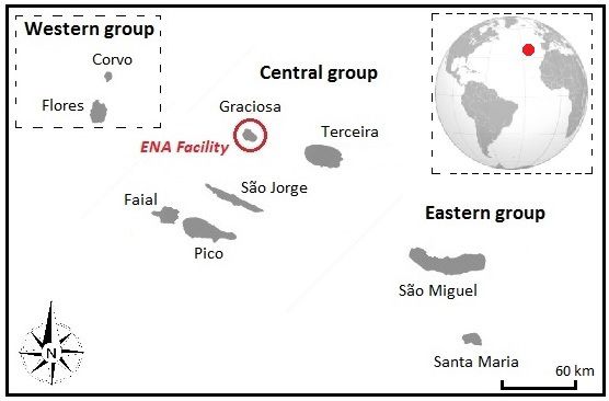
1 Representation of the Azores Archipelago together with the geographic location of ARM’s ENA
observatory on Graciosa Island (39º 03.12' N; 27º 57.10' W). ............................................................... 2
2 The JCI 131F field-mill installed at Graciosa, Azores. .......................................................................... 2
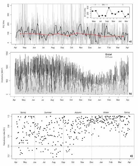
3 1-minute raw data of the (a) Potential Gradient (V/m) strict to the [0, 400] V/m interval, (b)
Global and Diffuse Irradiance (W/m2), and the (c) Nebulosity Index (Kn) on Graciosa Island. ............ 4
4 Daily averaged Potential Gradient (V/m) for each daily average nebulosity index Kn below 0.2,
0.3, 0.4, 0.5, and 0.6, together with the general Carnegie Curve (empty squares time series). .............. 5
5 Daily mean Potential Gradient, the corresponding Carnegie Curve, and the daily averaged AOD
for: (a) spring; (b) summer, and (c) autumn. .......................................................................................... 7
6 Weekly SST anomalies during ENSO (6 January 2010 to 27 July 2016). ............................................. 8
vHG Silva, July 2021, DOE/SC-ARM-21-013
1.0 Motivation
The foundation stone of atmospheric electricity is the existence of a Global Electric Circuit (GEC)
influencing all of the planet. In fact, global thunderstorm activity acts as a voltage source that imposes a
potential difference between the ionosphere (positively charged) and the Earth’s surface (negatively
charged) of about ~300 kV. Such potential difference is discharged through the poorly conducting
atmosphere in fair-weather regions, with atmospheric electric fields of ~100 V/m. First evidence of the
GEC was gathered by scientists involved on the Carnegie vessel expeditions (early 20th Century), in
which they describe a similar daily variation of the atmospheric electric field in different parts of the
Pacific Ocean. Such variation become known as the Carnegie Curve (CC).
Nevertheless, aerosols, mainly resulting from pollution, scavenge atmospheric ions and alter the
atmosphere’s electric properties (making it less conductive). This phenomenon tends to increase the
atmospheric electric field and makes it almost impossible to observe the features of the CC at inland
locations, especially if measurements are done near urban areas, which is the most common. For that
reason, not much research has been done on the CC since the expeditions.
With this in mind, the ARM field campaign, Atmospheric Electric Field-Mill Sensor
1HG Silva, July 2021, DOE/SC-ARM-21-013
Figure 1. Representation of the Azores Archipelago together with the geographic location of ARM’s
ENA observatory on Graciosa Island (39º 03.12' N; 27º 57.10' W).
The field-mill used for the local atmospheric electric field measurements, a JCI 131F (Chilworth, United
Kingdom), calibrated in December 2013, was installed at 2 m above ground (~31 m from sea level) and at
a horizontal distance of 500 m from the seashore. Moreover, this equipment has a flat spectral response
up to frequencies of ~100 Hz. A rate of 1-second sampling was used, with 1-minute mean and standard
deviation being performed and recorded.
Figure 2 presents a photograph of the installation at the ENA site.
Figure 2. The JCI 131F field-mill (Chilworth, United Kingdom) installed at Graciosa, Azores.
2HG Silva, July 2021, DOE/SC-ARM-21-013
3.0 Campaign and Data
This ARM-ENA campaign was designated as Atmospheric Electric Field-Mill Sensor, reference number
AFC06722. It started on September 1, 2014, and was meant to end on August 31, 2021. However,
high-quality data only started to be recorded by early 2015 and lasted until late 2020, when the field-mill
was unfortunately broken. More details can be found at www.arm.gov/campaigns/ena2014aefms
Data gathered by this instrument were included in the Global Coordination of Atmospheric Electricity
Measurements ( GLOCAEM) project, which intended to build a database for a network of measurement
sites across the world: https://glocaem.wordpress.com
Furthermore, the data were analyzed in two publications referenced below.
4.0 Results and Discussion
An initial assessment of the first year of measurements, starting on April 1, 2015, of the Potential
Gradient (PG) 1 on Graciosa Island is depicted in Figure 3. It should be noted that the results discussed in
this section are not representative of a long-term change, but can reveal a short-term response of the PG to
atmospheric phenomena. In Figure 3a, the raw data of the PG is presented, for the clarity of the
representation data is restricted to the range [0, 400] V/m (only ~3% data is out of the plot). Note the high
variability characteristic of these measurements. The oscillations can occur due to several local factors
such as nebulosity, rain, strong winds, space electrical charges, and even nearby insect or bird activity.
This reflects the high sensitivity of the measuring equipment and for that reason only data that comprise
fair-weather (FW) days were used further in the analysis; FW days are determined on the basis of the
nebulosity index (details given below). Moreover, in Figure 3a, a lowess smoothing curve (solid
blackline) is added to the plot as well as the average monthly PG values; these depict well the yearly
variation of the PG. Contrary to what is observed in urban environments, where there is a tendency for
lower PG values in the summer,[1] no clear annual tendency is observed in Graciosa, with the lower
monthly PG value being found for January (~ 64.4 V/m) and higher in October (~102.8 V/m). Monthly
PG variability (inset to Figure 2a) does seem to have some degree of seasonal tendency with summer
months having lower standard deviation (STD). Nevertheless, the lower STD was found in February
(~38.8 V/m) and the higher in September (~472.3 V/m). For the sake of clarity, seasons are separated:
spring comprises March, April, and May (MAM); summer includes June, July, and August (JJA); autumn
contains September, October, and November (SON); winter involves December, January, and February
(DJF). These definitions will be used subsequently.
1
Potential Gradient is related to the vertical component of the atmospheric electrical field, Ez, by the
formula PG = Ez. This guarantees positive values for the PG in fair-weather conditions.
3HG Silva, July 2021, DOE/SC-ARM-21-013
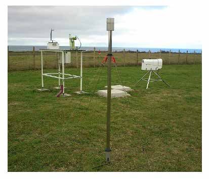
Figure 3. 1-minute raw data of the (a) Potential Gradient (V/m) strict to the [0, 400] V/m interval, (b)
Global and Diffuse Irradiance (W/m2), and the (c) Nebulosity Index (Kn) on Graciosa Island.
The solid black line in (a) represents a locally weighted scatterplot smoothing (lowess) curve
over the data and the defined PG interval is used to remove outliers that would make data
visualization difficult; the dots in that figure represent monthly averages and the inset the
monthly standard deviation.
Generically different hypotheses of both a local and global nature may be given to explain PG variability
throughout the year at Graciosa. Among the local phenomena that might affect the PG are: (1) the
atmospheric electric field can be charged or discharged due to the reduction or increase in the air
conductivity, respectively; (2) the influence of clouds, as these are charged and tend to increase the
PG.[2] The first hypothesis considers the variation of the air conductivity, which can occur by four
different mechanisms: (i) variation in the concentration of small marine ions brought by the sea breeze[3],
since the measurements are performed close to the sea (~500 m); (ii) the generation of space-charges due
to the burst of water droplets by wave splashing, the so called balloelectric effect[4 and references
therein]; (iii) variation of the local ionization by the variation of the emission rate of natural radioactive
gases, mainly radon;[5] (iv) reduction or increase of the small ions concentration by an increased or
reduced scavenging of the existing ions by water droplets and hygroscopic particles,[6] respectively.
4HG Silva, July 2021, DOE/SC-ARM-21-013
In terms of global effects, the PG values tend to increase or decrease as a result of addition or reduction in
the charging of the GEC, respectively, by generators, mainly lightning. The present results do not show a
clear seasonality of GEC, in line with the work of Tacza and co-authors[7] who, when analyzing three
years of PG data in South America stations, noted that the average daily shape during a month, season, or
year repeats similarly for different years, supporting the results here presented. This is in contradiction
with the seasonal variations observed in the Carnegie expedition data.[8]
Moreover, the analysis for the diurnal variation shows that the PG can be affected by different factors
throughout the day. The criteria applied for the selection of the FW days was established on the
nebulosity index (Kn), which is defined as the ratio between the diffuse (Ed) and global (Eg) horizontal
irradiances (Figure 3b):
where the index typically goes from 1 for overcast-sky to ~0.2 in clear-sky conditions. It should be said
that radiation measurements are also done at the ENA site. Equation 1 is a simplification of the
Perraudeau nebulosity index.[9] The obtained 1-day Kn is depicted in Figure 3c. To apply the nebulosity
index in the FW selection, a number of different Kn were considered (Figure 4). The results show a
diverse number of FW days and the corresponding average daily PG for each Kn obtained is shown in
Figure 4. The nebulosity index that was selected for further analysis was for Kn < 0.4, as a trade-off of a
statistically representative sample (28 days) and a smooth variation of the average daily PG curve (low
relative standard deviation). PG curves for Kn < 0.5 and Kn < 0.6 are not suitable for FW criteria since
they show sharp oscillations between 4 and 6 UTC that might be attributed to disturbed weather
conditions. Additionally, an inset with the relative standard deviation (%) for each PG curve
corresponding to different Kn is also depicted in Figure 4, as it was obtained through:
The inset plot in Figure 4 shows that the selected nebulosity index (Kn < 0.4) presents the best
combination between a low relative standard deviation (i.e., a smooth variation from the mean value) and
significant statistical samples (in this case, 28 FW days).
Figure 4. Daily averaged Potential Gradient (V/m) for each daily average nebulosity index Kn below
0.2, 0.3, 0.4, 0.5, and 0.6, together with the general Carnegie Curve (empty squares time
series). Error bars are added to the PG curve corresponding to the 0.4 nebulosity index, while
the inset shows the relative standard deviation (%) for each PG curve.
5HG Silva, July 2021, DOE/SC-ARM-21-013
A deviation from the Carnegie Curve is observed in the FW PG daily mean curve: lower values with a
more pronounced increase in the late morning hours (7 to 10 UTC) and a smooth variation during the
afternoon. Additionally, a correlation of ~0.71, with a pvalue < 0.0001, was found between the selected
Graciosa PG curve (marked in black) and the Carnegie Curve. The overall lower PG values, as compared
with the Carnegie Curve, could be either related to instrumentation or to local effects. One possible local
effect is ionization created by natural radioactive gases (radon) that is present over land, but absent in the
ocean environment. It is commonly accepted that the two main sources of atmospheric ionization are
cosmic rays and radon. To this can be added breaking waves near the seaside;[10,11] this is the case on
Graciosa Island. In fact, being a volcanic island might as well promote radon migration from the Earth’s
surface.[12] Co-located measurements of radon are now being made and future analysis will consider
both radon and PG together to explore this suggestion.[12] In the case of measurements in the open ocean
like the ones done by the Carnegie[8] and other cruises,[13] the only source of ionization is cosmic rays
and for that reason lower air conductivity is observed there,[13] and as a consequence of Ohm’s law the
PG is higher. The presence of natural radioactivity is possibly one of the main differences between the
conditions in which the Carnegie Curve was measured and the measurements made in Graciosa Island.
Another possibility is the presence of marine ions, as the Carnegie Curve results from measurements
taken aboard ships, where there are no breaking waves, contrary to Graciosa, where waves break all along
the coastline, allowing the generation of many marine ions. These ions are highly mobile and tend to
discharge the local electric field by increasing air’s conductivity. This effect has been reported[10] such
that when the wind came directly from the sea, there was a greater influence of marine air and the air
tended to rise in conductivity.
A closer look into the data, applying the same nebulosity index criteria, but dividing the data into seasons
spring (MAM); summer (JJA); autumn (SON); winter (DJF) showed the existence of 8 FW days for
spring, 14 FW days for summer, 6 FW days for autumn, and none for winter. The mean daily PG curves
and corresponding Carnegie Curves (CC) (obtained from parameters estimated by [8]) for each season are
shown in Figures 5a, b, and c. In these plots, we added the mean daily aerosol optical depth (AOD)
behavior for the corresponding days of FW used in the PG calculations for each season. Generally, the
summer tends to show lower values of AOD coinciding with a better agreement between the PG and CC
curves for this season. This could indicate the role that aerosols, as a local effect, might have in the
deviation of the measured PG from the signal imposed by the global modulation of the electric field as
uttered by the CC.
6HG Silva, July 2021, DOE/SC-ARM-21-013
Figure 5. Daily mean Potential Gradient, the corresponding Carnegie Curve, and the daily averaged
AOD for: (a) spring; (b) summer, and (c) autumn. Left y-axis corresponds to the PG and the
right y-axis to the AOD (440 nm).
Comparing the PG curves in the three seasons, we see that they have similar behavior, showing the
expected minima at dawn and the maxima in the evening (in conformity to the minima and maxima
observed in CC for each season). The small contrasts observed are probably due to the fact that the PG
measurements at Graciosa are more sensitive to thunderstorms in America, Europe, and Africa than to
those in Asia and Australia. In the first three regions, thunderstorm activity tends to have its minima later
in comparison with the last two ones.[8] In terms of the daily PG maxima, they occur at 18 UTC in spring
(second dashed line in the plots), 19-20 UTC in the summer (dotted line in the plots), and 18-19 UTC in
autumn. This is approximately one hour earlier than the CC references that have their maxima at
7HG Silva, July 2021, DOE/SC-ARM-21-013
19-20 UTC, 21-22 UTC, and 19 UTC, respectively, for spring, summer, and autumn. This shows that the
seasonal change in the time of occurrence of the afternoon PG maximum at Graciosa is consistent with
the change of the maximum of the CC references (Figures 5a, b, and c), though the CC maxima occur
around one hour later. The fact that PG maxima are recorded earlier in Graciosa Island also suggests the
possible influence of the proximity of the European and African continents, where thunderstorm activity
peaks are attained around 13 UTC; while American thunderstorm activity peaks around 19 to 20 UTC.[8]
In this context, the effect of the strong 2015 El Niño should help in understanding the seasonal change in
the time of occurrence of the PG maximum at Graciosa. In Figure 6 large positive weekly sea surface
temperature (SST) anomalies in the Eastern Pacific, Niño 1+2 (0-10° South, 90°-80° West) and Niño 3
(5° North-5°South, 150° -90° West), are clearly identified for 2015, depicting a strong increase during the
spring (dashed vertical line) and summer (pointed vertical line) months. El Niño-Southern Oscillation
(ENSO) data from 6 January 2010 to 27 July 2016 here presented was retrieved from the National
Oceanic and Atmospheric Administration (NOAA)’s website (www.cpc.ncep.noaa.gov). El Niño is
known to affect the global distribution of thunderstorms, shifting Pacific thunderstorms eastward,
increasing the relevance of the American thunderstorms peak in Graciosa Island. In fact, there is a growth
in the intensity of thunderstorm activity between spring and summer over North America[14] that results
from the ENSO strengthening that has been occurring since 1996. Comparison with La Niña years will be
done in the future.
Figure 6. Weekly SST anomalies during ENSO (6 January 2010 to 27 July 2016). Vertical dashed lines
mark the beginning of spring and summer seasons during 2015 for El Niño 1+2 (0-10S,
90-80W) and El Niño 3 (5N-5S, 150-90W). The depicted data is available online and can be
retrieved from: www.cpc.ncep.noaa.gov/data/indices/wksst8110.for
On the other hand, the first vertical dashed lines mark the observed PG increase during the morning
(around 9-10 UTC) for the three curves in Graciosa, but not observed in the Carnegie reference curves
that show a smooth increase from the dawn minima to the evening maxima. This deviation of the diurnal
Graciosa PG from the CC during the late morning is difficult to interpret in the context of the GEC. Such
deviation is expected to be due to near-surface aerosol generated in the island after sunrise, which would
reduce the air conductivity in the morning. In some respect, this is a feature common to inland stations in
which it is often observed as a double maximum: (1) in the morning, due to the rise of near-surface
aerosols; (2) in the evening, due to the GEC. This behavior is particularly clear for the spring and autumn
PG curves in Graciosa, Figures 5a and c. Nevertheless, the mean AOD values, also measured at the ENA
8HG Silva, July 2021, DOE/SC-ARM-21-013
site, for that time (9-10 UTC) of the day are low (0.15, 0.08, 0.15 for spring, summer, autumn,
respectively), corresponding essentially to clean aerosol conditions according to the definition given
by[15]: AOD (440 nm) < 0.12. More interesting is the fact that in the period from 10 UTC to 16-17 UTC,
while there are relatively high values of AOD, the PG seems to suffer a reduction. In fact, there seems to
be an AOD peak (13 UTC in spring and 15 UTC in summer and autumn, reaching 0.65, 0.15, and 1.65,
respectively, for each season) accompanied by a PG minimum one to three hours later (16 UTC in spring,
17 UTC in summer, and 16 UTC in autumn, with PG values of 107.7, 98.9, 81.4 V/m, respectively, for
each season). Since the AOD data have large standard deviations (not shown here), their relevance to the
PG analysis should be considered with particular care.
Nevertheless, the only possibility that can be inferred to explain these observations is that the AOD
measurements are measuring aerosols mixed with some sort of charge carriers (which are not accessible
to AOD) that would tend to increase the atmospheric electric conductivity (reduce PG), balancing the
aerosol effect that is, to reduce atmospheric electric conductivity (increase PG). The measurements are
made at the seaside and according to the observations made in similar sites[10,11] the influence of marine
ions can be hypothesized to explain the observations. Many studies can be found in the literature
dedicated to the formation of space-charge distributions (basically the imbalance between positive and
negative small ion clusters) at seaside locations[16,17,18] that might support the present hypothesis. The
typical marine cations are H+, NH4+, Na+, Mg2+, K+, Ca2+ and anions are NO3-, Cl-, SO42-, HCO3-[19]
Although they should be hydrated by water molecules while remaining in the atmosphere, these ions have
high electric mobilities and should, for that reason, increase the atmospheric electric conductivity and, as
a consequence of Ohm’s law, they should therefore reduce the PG.[10] For this to explain the reduction of
the PG while observing a peak in the AOD means that the concentration of marine ions has to be
significant. A simple estimation of the amount of space-charge needed for the observed PG minimum can
be made for the autumn using the Carnegie value as reference, 141.9 V/m, and the measured PG,
81.4 V/m, at 16 UTC. The difference of the two values is ~60.5 V/m, which if attributed to the
space-charge created by the marine ions, allows the use of Equation 8 from [20] (assuming similar
parameters) to estimate the space-charge to be nearly ~103 pC/m3; which is a very reasonable value
indeed.[20,21] Taking into account that waves break all along the seashore of the island (with a power
around ~20-30 kW/km of wave front), it is easy to understand that those marine ions are constantly being
sprayed into the atmosphere. The concentrations can be higher in more convective situations, as is the
case for the midday. The same happens for marine aerosols explaining the midday AOD peak, even
though the effect of the marine ions on the PG should be prolonged since these ions have large
characteristic times of recombination (well above the ~20 s for polluted regions), as this is a very
low-pollution environment. After 19 UTC the AOD is again below or near to the 0.12 threshold for clean
aerosol conditions and the GEC signal is recovered as it is revealed by the evening maxima in the PG
curves for the three seasons (Figures 5a, b, and c), as previously discussed.
In short, unlike the Carnegie cruise expeditions, which were entirely ocean based, Graciosa is an island,
so it will experience wave-break and wind-blown aerosols and ions in the immediate vicinity of the
electric field-mill (~500 m from the shore). This means that the local effects of increased aerosol and ion
concentrations after sunrise until sunset are still observed, causing the PG to depart from the GEC signal
and approach that of an inland situation. Still, before sunrise and after sunset, the PG at Graciosa tends to
reproduce the CC behavior very well, making this period suitable for GEC research.
9HG Silva, July 2021, DOE/SC-ARM-21-013
5.0 Conclusions
For the first time, measurements of the atmospheric electric field have been carried out at the ARM-ENA
facility on Graciosa Island (Azores archipelago) as part of a network effort for the study of the Global
Electrical Circuit variability. Results show that under fair-weather conditions, the island’s Potential
Gradient is locally affected by marine air. These conditions tend to alter the diurnal Potential Gradient
away from the Carnegie towards that seen at land sites. On a global scale, Graciosa Island appears to be a
good place for the study of the GEC because signatures of large-scale systems such as ENSO are
apparently observed in the seasonal changes of Potential Gradient.
Further work would have to be dedicated to the analysis of the remaining years of data, from which very
promising results are expected. These could not only provide new perspectives on the Global Electric
Circuit recent evolution, but also motivate new field campaigns.
6.0 References
[1] Silva, HG, R Conceição, M Melgão, K Nicoll, PB Mendes, M Tlemçani, AH Reis, and RG Harrison.
2014. “Atmospheric electric field measurements in urban environment and the pollutant aerosol weekly
dependence.” Environment Research Letters 9(11): 114025, https://doi.org/10.1088/1748-
9326/9/11/114025
[2] Nicoll, KA, and RG Harrison. 2010. “Experimental determination of layer cloud edge charging from
cosmic ray ionisation.” Geophysical Research Letters 37(13): L13802,
https://doi.org/10.1029/2010GL043605
[3] Silva, HG, JC Matthews, R Conceição, MD Wright, SN Pereira, AH Reis, and DE Shallcross. 2015.
“Modulation of urban atmospheric electric field measurements with the wind direction in Lisbon
(Portugal).” Journal of Physics: Conference Series 646: 012013, https://doi.org/10.1088/1742-
6596/646/1/012013
[4] Tammet, H, U Hõrrak, and M Kulmala. 2009. “Negatively charged nanoparticles produced by
splashing of water.” Atmospheric Chemistry and Physics 9(2): 357–367, https://doi.org/10.5194/acp-9-
357-2009
[5] Lopes, F, HG Silva, S Bárias, and SM Barbosa. 2015. “Preliminary results on soil-emitted gamma
radiation and its relation with the local atmospheric electric field at Amieira (Portugal).” Journal of
Physics: Conference Series 646, 012015, https://doi.org/10.1088/1742-6596/646/1/012015
[6] Silva, HG, R Conceição, MD Wright, JC Matthews, S. Pereira, and DE Shallcross. 2015. “Aerosol
hygroscopic growth and the dependence of atmospheric electric field measurements with relative
humidity.” Journal of Aerosol Science 85: 42 51, https://doi.org/10.1016/j.jaerosci.2015.03.003
[7] Tacza, J, J-P Raulin, E Macotela, E Norabuena, G Fernandez, E Correia, MJ Rycroft, and
RG Harrison. 2014. “A new South American network to study the atmospheric electric field and its
variations related to geophysical phenomena.” Journal of Atmospheric and Solar-Terrestrial Physics
120: 70–79, https://doi.org/10.1016/j.jastp.2014.09.001
10HG Silva, July 2021, DOE/SC-ARM-21-013
[8] Harrison, RG. 2013. “The Carnegie Curve.” Surveys in Geophysics 34: 209 232,
https://doi.org/10.1007/s10712-012-9210-2
[9] Perraudeau, M, and P Chauvel. 1986. “One year’s measurements of luminous climate in Nantes.”
Proceedings of the International Daylighting Conference, Long Beach, California.
[10] Wilding, RJ, and RG Harrison. 2005. “Aerosol modulation of small ion growth in coastal air.”
Atmospheric Environment 39(32): 5876–5883, https://doi.org/10.1016/j.atmosenv.2005.06.020
[11] Reiter, R. 1994. “Charges on particles of different size from bubbles of Mediterranean Sea surf and
from waterfalls.” Journal of Geophysical Research – Atmospheres 99(D5):10807 10812,
https://doi.org/10.1029/93JD03268
[12] Barbosa, SM, P Miranda, and EB Azevedo. 2017. “Short-term variability of gamma radiation at the
ARM Eastern North Atlantic facility (Azores).” Journal of Environmental Radioactivity 172: 218 231,
https://doi.org/10.1016/j.jenvrad.2017.03.027
[13] Kamra, AK, CG Deshpande, and V Gopalakrishnam. 1997. “Effect of relative humidity on the
electrical conductivity of marine air.” Quarterly Journal of the Royal Meteorological Society
123(541): 1295 1305, https://doi.org/10.1002/qj.49712354108
[14] Christian, HJ, RJ Blakeslee, DJ Boccippio, WL Boeck, DE Buechler, KT Driscoll, SJ Goodman,
JM Hall, WJ Koshak, DM Mach, and MF Stewart. 2003. “Global frequency and distribution of lightning
as observed from space by the Optical Transient Detector.” Journal of Geophysical Research –
Atmospheres 108(D1): ACL 4-1 ACL4-15, https://doi.org/10.1029/2002JD002347
[15] Elias, T, AM Silva, N Belo, S Pereira, P Formenti, G Helas, and F Wagner. 2006. “Aerosol
extinction in a remote continental region of the Iberian Peninsula during summer.” Journal of
Geophysical Research 111: D14204, https://doi.org/10.1029/2005JD006610
[16] Blanchard, DC. 1966. “Positive Space Charge from the Sea.” Journal of the Atmospheric Sciences
23(5): 507 515, https://doi.org/10.1175/1520-0469(1966)0232.0.CO;2
[17] Gathman, SG, and WA Hoppel. 1970. “Surf electrification.” Journal of Geophysical Research
75(24): 4525 4529, https://doi.org/10.1029/JC075i024p04525
[18] Muir, MS. 1977. “Atmospheric electric space charge generated by the surf.” Journal of Atmospheric
and Terrestrial Physics 39(11-12): 1341 1346, https://doi.org/10.1016/0021-9169(77)90086-1
[19] Lonso, R, G Bergametti, P Carlier, and G Mouvier. 1991. “Major ions in marine rainwater with
attention to sources of alkaline and acidic species.” Atmospheric Environment. Part A. General Topics
25(3-4): 763 770, https://doi.org/10.1016/0960-1686(91)90074-H
[20] Lopes, F, HG Silva, R Salgado, M Potes, KA Nicoll, and RG Harrison. 2016. “Atmospheric
electrical field measurements near a fresh water reservoir and the formation of the lake breeze.” Tellus A
68(1): 31592, https://doi.org/10.3402/tellusa.v68.31592
11HG Silva, July 2021, DOE/SC-ARM-21-013
[21] Harrison, RG, and KS Carslaw. 2003. “Ion-aerosol-cloud processes in the lower atmosphere.”
Reviews of Geophysics 41(3): 1012, https://doi.org/10.1029/2002RG000114
7.0 Publications Related to the Campaign
1. Lopes, F, HG Silva, AJ Bennett, and AH Reis. 2017. “Global Electric Circuit research at Graciosa
Island (ENA-ARM facility): First year of measurements and ENSO influences.” Journal of
Electrostatics 87: 203 211, https://doi.org/10.1016/j.elstat.2017.05.001
2. Nicoll, KA, RG Harrison, V Barta, J Bor, R Brugge, A Chillingarian, J Chum, AK Georgoulias, A
Guha, K Kourtidis, M Kubicki, E Mareev, J Matthews, H Mkrtchyan, A Odzimek, J-P Raulin, D
Robert, HG Silva, J Tacza, Y Yair, and R Yaniv. 2019. “A global atmospheric electricity
monitoring network for climate and geophysical research.” Journal of Atmospheric and Solar-
Terrestrial Physics 184: 18–29, https://doi.org/10.1016/j.jastp.2019.01.003
12You can also read