Axisymmetric Hydrodynamics in Numerical Relativity Using a Multipatch Method
←
→
Page content transcription
If your browser does not render page correctly, please read the page content below
Axisymmetric Hydrodynamics in Numerical Relativity
                                        Using a Multipatch Method
                                                Jerred Jesse1 , Matthew D. Duez1 F. Foucart2 , Milad Haddadi1 ,
                                                Alexander L. Knight2 , Courtney L. Cadenhead1 , Francois Hébert3 ,
arXiv:2005.01848v2 [gr-qc] 2 Jul 2020

                                                Lawrence E. Kidder4 , Harald P. Pfeiffer5 , Mark A. Scheel3
                                                1
                                                  Department of Physics & Astronomy, Washington State University, Pullman, Washington
                                                99164, USA
                                                2
                                                  Department of Physics & Astronomy, University of New Hampshire, 9 Library Way,
                                                Durham NH 03824, USA
                                                3
                                                  TAPIR, Walter Burke Institute for Theoretical Physics, MC 350-17, California Institute of
                                                Technology, Pasadena, California 91125, USA
                                                4
                                                  Center for Radiophysics and Space Research, Cornell University, Ithaca, New York, 14853,
                                                USA
                                                5
                                                  Max-Planck-Institut fur Gravitationsphysik, Albert-Einstein-Institut, D-14476 Golm,
                                                Germany

                                                Abstract. We describe a method of implementing the axisymmetric evolution of general-
                                                relativistic hydrodynamics and magnetohydrodynamics through modification of a multipatch
                                                grid scheme. In order to ease the computational requirements required to evolve the post-
                                                merger phase of systems involving binary compact massive objects in numerical relativity, it
                                                is often beneficial to take advantage of these system’s tendency to rapidly settle into states that
                                                are nearly axisymmetric, allowing for 2D evolution of secular timescales. We implement this
                                                scheme in the Spectral Einstein Code (SpEC) and show the results of application of this method
                                                to four test systems including viscosity, magnetic fields, and neutrino radiation transport. Our
                                                results show that this method can be used to quickly allow already existing 3D infrastructure
                                                that makes use of local coordinate system transformations to be made to run in axisymmetric
                                                2D with the flexible grid creation capabilities of multipatch methods. Our code tests include a
                                                simple model of a binary neutron star postmerger remnant, for which we confirm the formation
                                                of a massive torus which is a promising source of post-merger ejecta.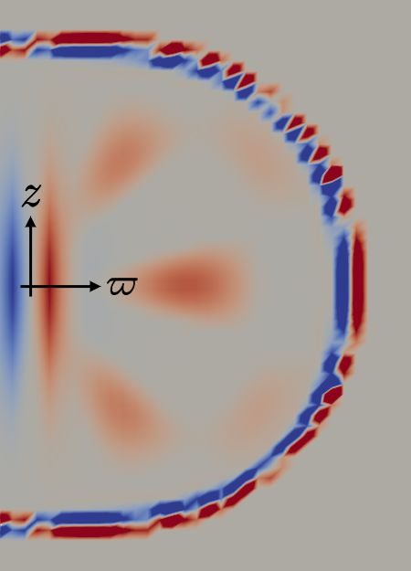
Axisymmetric Hydrodynamics in Numerical Relativity Using a Multipatch Method                 2

1. Introduction

The detection of the gravitational wave signal resulting from the merger binary black hole
systems by the LIGO and VIRGO collaborations [1, 2, 3, 4, 5, 6, 7] along with the detection of
simultaneous electromagnetic and gravitational wave signals from binary neutron star mergers
[8, 9, 10, 11], and the corresponding need for theoretical predictions with which to compare
them, has given renewed urgency to the goal of accurately modeling these systems throughout
the merger process. For systems involving at least one neutron star, it is the post-merger
state that is primarily responsible for the observable electromagnetic signals. Modeling
of these systems through numerical relativity simulations provides critical insight into the
dependencies of the signals on binary parameters and nuclear physics. Unfortunately, running
these simulations in the high-resolution required to get accurate predictions can present
large computational resource barriers in simulated time or size scales. However, the post-
merger environment has a useful property: by taking advantage of these systems’ tendency to
approach an axisymmetric state, we can ease the computational resources required to simulate
these systems over extended scales of both time and space. Although the dynamical timescales
of remnant neutron stars and accretion disks, of the order ∼ms at most, are reasonably
accessible to 3D simulations, secular effects that drive the subsequent evolution can operate
on much longer timescales. Particularly important are angular momentum transport effects
that can act on a wide range of timescales of up to hundreds of milliseconds [12, 13], and
neutrino cooling effects that operate on timescales of up to several seconds [14].
     The use of axisymmetry in numerical relativity simulations has been explored by several
groups. This typically involves evolving Einstein’s equations using the cartoon method [15]
while evolving hydrodynamics by writing the relevant equations in a cylindrical coordinate
system [16, 17, 18]. The cartoon method does involve some loss of accuracy due to
interpolations required in the method, and some effort has been made to avoid these [19].
Additionally, evolution problems due to the coordinate singularities that arise from the use
of polar coordinate systems have been avoided by use of a reference metric [20, 21, 22].
Methods also exist that help with issues of spatial resolution on large scales, such as
adaptive mesh refinement [19, 23], which is able to concentrate resolution where it is most
needed, while in most cases still building the grid from Cartesian domains. In multipatch
methods [24, 25, 26, 27, 28, 29], one introduces coordinate patches, each with its own local
coordinate system in which it takes a simple shape (e.g. a Cartesian block), but which
can be deformed in the global coordinate system and fit together into a grid to match the
geometry of the problem. A number of methods used in numerical relativity not usually
called “multipatch” have local coordinate systems and therefore fit into this general category,
including the multidomain pseudospectral sector of the Spectral Einstein Code [30] and the
multielement discontinuous Galerkin methods [31, 32] which many hope will form the basis
of the next generation of numerical relativity codes.
     In this paper, we describe a method of implementing the axisymmetric evolution of the
general-relativistic equations of ideal radiation hydrodynamics and magnetohydrodynamics
through modification of a multipatch grid scheme, applicable to any method using the local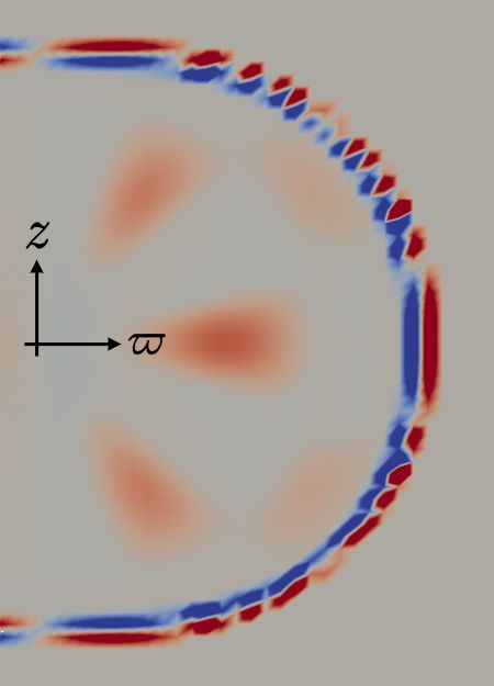
Axisymmetric Hydrodynamics in Numerical Relativity Using a Multipatch Method                  3

patch coordinates framework, which we implement in the Spectral Einstein Code (SpEC) [30].
While other codes for carrying out axisymmetric relativistic hydrodynamics evolutions exist,
there are several notable new features of our methods and results. First, using the multipatch
framework, we automate the conversion to an axisymmetry-friendly coordinate system, which
we demonstrate by using the same recipe to make working axisymmetric 2D versions of
our relativistic 3D hydrodynamics, magnetohydrodynamics, neutrino transport, and shear
viscosity codes. We point out that our neutrino transport method, which evolves number
density as well as energy density, is somewhat different from other grey M1 schemes, so
this is the first time this particular system has been converted to 2D axisymmetry. Second,
we inherit the flexibility of multipatch methods to construct grids from patches of different
shapes to optimally match the geometry of a problem. As a demonstration of this, we present
the 2D evolution of a viscous differentially rotating star using a combination of square patches
for the stellar interior and circular wedges for the outflow zone. As well as serving as a
code test, this viscous rotating star system is of great astrophysical interest because it is a
reasonable model of the remnant of a binary neutron star merger. We evolve it using a different
subgrid momentum transport model than has been applied to it in prior work [33], providing
an important qualitative check on the previous results. Finally, we present several minor
enhancements of the SpEC-Hydro code, including a generalization of our auxiliary entropy
evolution [29] to the thermal Gamma-law class of equations of state an altered form of the
divergence cleaning magnetohydrodynamics equations, and an altered treatment of neutrino
fluxes in the optically thick limit.
      This paper is organized as follows. In Sec. 2, we describe the evolution equations for our
(magneto)hydrodynamic variables and the application of our axisymmetry method to them.
In Sec. 3 several tests of this axisymmetry method are presented: a stationary TOV star,
a viscous differentially rotating star, a magnetized accretion disk, and neutrino radiation in
a spherically symmetric supernova collapse profile, each showing good agreement with 3D
results or previous axisymmetric simulations. Concluding remarks are given in Sec. 4, where
we summarize our results and discuss future plans.

2. Formulation

2.1. Evolution Equations

We use SpEC to evolve Einstein’s equations and the general relativistic equations of ideal
radiation (magneto)hydrodynamics. SpEC evolves Einstein’s equations and the general
relativistic hydrodynamics equations on two separate computational grids. A multidomain
grid of colocation points is used to evolve Einstein’s equations pseudospectrally in a
generalized harmonic formulation [34] while the general relativistic (magneto)hydrodynamics
equations in conservative form are evolved on a finite difference grid. The finite difference
grid uses an HLL approximate Riemann solver [35]. Reconstruction of values at cell faces
from their cell-average values is done using a high-order shock capturing method, a fifth-
order WENO scheme [36, 37]. Time evolution is performed using a third-order Runge-Kutta
Axisymmetric Hydrodynamics in Numerical Relativity Using a Multipatch Method 4
algorithm with an adaptive time-stepper. At the end of each time step any necessary source
term information is then communicated between the two grids, using a third-order accurate
spatial interpolation scheme [38].
The following sections make use of the 3+1 decomposition of the spacetime metric
ds2 = gαβ dxα dxβ (1)
2 2
dx + β dt dxj + β j dt ,
i i
= − α dt + γij (2)
where α is the lapse, β i the shift, and γij is the three-metric on a spacelike hypersurface of
constant coordinate t. The three-metric is the projection onto spatial hypersurfaces of the
four-metric:
γij = gij + ni nj , (3)
where nµ = (−α, 0, 0, 0) is the unit normal to the t = constant hypersurface. Additionally,
we use the units with G = c = 1 throughout.
2.1.1. Fluid We begin by treating our fluid as a perfect fluid with the stress-energy tensor
Tµν = ρ0 huµ uν + P gµν , (4)
where ρ0 is the baryon density, h = 1 + P/ρ0 + is the specific enthalpy, P is the pressure,
uµ the four-velocity, and the specific internal energy.
The general relativistic hydrodynamics equations are evolved using the conservative
variables
√ √
ρ∗ = − γnµ nν ρ0 = ρ0 W γ, (5)
√ µν √
τ = γnµ nν T − ρ∗ = ρ∗ (hW − 1) − P γ, (6)
√ µ
Si = − γnµ Ti = ρ∗ hui , (7)
p
where W = 1 + γ ij ui uj is the Lorentz factor and γ is the determinant of γij . Using
conservation of energy and momentum, ∇ν T µν = 0, and baryon number conservation,
∇µ (ρ0 uµ ) = 0, we get the evolution equations for the conservative variables:
∂t ρ∗ + ∂j ρ∗ vTj = 0,
(8)
√ √
∂t τ + ∂j α2 γT 0i − ρ∗ vT i = −α γT µν ∇µ nν ,
(9)
√ 1 √
∂t Si + ∂j α γTi j = α γT µν ∂i gµν ,
(10)
2
where the Eulerian velocity v i is related to the fluid transport velocity vT i by vT i = αv i − β i .
Additionally, for simulations involving nuclear matter and neutrinos, we evolve the electron
fraction of the fluid, Ye ,
∂t (ρ∗ Ye ) + ∂j ρ∗ Ye vTj = 0.
(11)
To close these equations we must also supply an equation of state for the pressure and
enthalpy: P = P (ρ∗ , T, Ye ) and h = h(ρ∗ , T, Ye ).Axisymmetric Hydrodynamics in Numerical Relativity Using a Multipatch Method 5
2.1.2. Magnetic Fields To handle magnetic fields, we begin by adding the electromagnetic
contribution, TEM µν , to the fluid stress-energy tensor, where
1
TEM µν = F µα F να − Fαβ F αβ g µν , (12)
4
and F µν is the Faraday tensor. We treat the fluid as a perfect conductor, F µν uν = 0, which
gives a fixed electric field for a given magnetic field.
We use two different methods for evolving the magnetic field, as described in [29]. The
first method evolves the magnetic vector potential Ai and scalar potential Φ. In the generalized
Lorentz gauge [39], the most robust gauge choice we have explored, the evolution equations
are
∂t Ai + ∂i αΦ − β j Aj = ijk v j B k ,
(13)
√ √ j √ j √
∂t ( γΦ) + ∂j α γA − γβ Φ = − ξα γΦ, (14)
where ξ is a specifiable constant of the order of the mass of the system.
The second method evolves the magnetic field using a covariant hyperbolic divergence
cleaning method [40, 41, 42] in which an auxiliary scalar evolution variable Ψ is introduced
in order to propagate and damp monopole formation. In this method, the induction equation
takes the form
∂t B̃ − ∂i v B̃ − v B̃ = αγ ij ∂j Ψ̃ + β i ∂j B̃ j ,
i j i i j
(15)
∂t Ψ̃ + ∂i αB̃ i − β i Ψ̃ = B̃ i ∂i α − α K ii + λ Ψ̃,
(16)
√ √
where B̃ i = γB i , Ψ̃ = γΨ, K ii is the trace of the extrinsic curvature, and λ is a specifiable
damping constant. Previously [29], we had used Ψ rather than Ψ̃ as an evolution variable, but
we find the new choice to be slightly more robust near excision inner boundaries.
2.1.3. Neutrinos Neutrino evolution is handled using the gray two-moment scheme as
described in [43, 44]. This method provides evolution of neutrino average energy densities,
flux densities, and number densities. We define three neutrino species that we evolve: electron
neutrinos νe , electron antineutrinos ν̄e , and the heavy lepton neutrinos νx . The heavy lepton
neutrino species groups together the four heavy lepton neutrinos and antineutrinos: νµ , ν̄µ , ντ ,
and ν̄τ .
We can describe each of our three species of neutrinos νi using each species’ distribution
function fν (xµ , pµ ), where xµ = (t, xi ) gives the time and position of the neutrinos and pµ
is the 4-momentum of the neutrinos. fν evolves in phase space according to the Boltzmann
transport equation:
α ∂f(ν) β γ ∂f(ν)
p − Γ αγ p = C f(ν) , (17)
∂xα ∂pβ
where the term C f(ν) includes all collisional processes (emissions, absorptions, and
scatterings).
We simplify the radiation evolution by taking the gray approximation (integrating over
the neutrino spectrum) and evolving the lowest two moments of the distribution functionsAxisymmetric Hydrodynamics in Numerical Relativity Using a Multipatch Method 6
of each neutrino species, truncating the moment expansion by imposing the Minerbo
closure [45]. Our evolved quantities are projections of the stress-energy tensor of the neutrino
radiation, Trad µν . The decomposition of Trad µν in the fluid frame is
Trad µν = Juµ uν + H µ uν + H ν uµ + S µν (18)
with H µ uµ = S µν uµ = 0. The energy density J, flux density H µ , and stress density S µν
of the neutrino radiation as observed in the frame comoving with the fluid are related to the
distribution functions by
Z ∞ Z
3
J = dν ν dΩ f(ν) (xα , ν, Ω) , (19)
0
Z ∞ Z
µ 3
H = dν ν dΩ f(ν) (xα , ν, Ω) lµ , (20)
Z0 ∞ Z
S µν = dν ν 3 dΩ f(ν) (xα , ν, Ω) lµ lν , (21)
0
R
where ν is the neutrino energy in the fluid frame, dΩ denotes integrals over solid angle in
momentum space, and
pα = ν (uα + lα ) , (22)
where lα uα = 0 and lα lα = 1. We also make use of the decomposition of the neutrino
radiation stress-energy tensor as observed by a normal observer,
Trad µν = Enµ nν + F µ nν + F ν nµ + P µν , (23)
with F µ nµ = P µν nµ = F t = P tν = 0. Additionally, for each species of neutrino we consider
the number current density:
N µ = N nµ + F µ , (24)
where N is the neutrino number density, and F µ is the number density flux. The
decomposition of N µ relative to the fluid frame can be expressed in terms of J, H µ , and
the fluid-frame average neutrino energy hνi as
Juµ + H µ
Nµ = . (25)
hνi
We define a projection operator onto the reference frame of an observer comoving with
the fluid,
hαβ = gαβ + uα uβ . (26)
This allows us to then use the fluid-frame variables to write equations for the energy, flux, and
stress tensor in the normal frame (i.e. the frame with 4-velocity equal to the normal vector)
E = W 2 J + 2W vµ H µ + vµ vν S µν , (27)
= W 2 vµ J + W gµν − nµ vν H ν
Fµ (28)
ν νρ
+ W vµ vν H + gµν − nµ vν vρ S ,
= W vµ vν J + W gµρ − nµ vρ vν H ρ
2
Pµν (29)
+ gµρ − nµ vρ (gνκ − nν vκ ) S ρκ
+ W gρν − nρ vν vµ H ρ ,
Axisymmetric Hydrodynamics in Numerical Relativity Using a Multipatch Method                      7

by making use of the decomposition of the 4-velocity, uµ = W (nµ + v µ ).
                                      √             √                    √
    Evolution equations for Ẽ = γE, F̃ i = γF i , and Ñ = γN can then be written in
conservative form:

               ∂t Ẽ + ∂j αF̃ j − β j Ẽ =                                       (30)

                        α P̃ ij Kij − F̃ j ∂j ln α − S̃rad
                                                        α
                                                           nα

               ∂t F̃i + ∂j αP̃i j − β j F̃i =                                    (31)
                                              α
                      − Ẽ∂i α + F̃k ∂i β k + P̃ jk ∂i γjk + αS̃rad
                                                                α
                                                                    γiα ,
                            √                2     √
               ∂t Ñ + ∂j α γF j − β j Ñ = α γC(0) ,                            (32)
               √
where P̃ij = γPij . Complete treatment of these equations requires prescriptions for the
closure relation that computes P ij (E, Fi ), the computation of F j and the collisional source
        α
terms S̃rad and C(0) which couple the neutrinos to the fluid (and introduce corresponding
source terms to the right hand side of Eq. 9, 10, and 11). Details on the treatment for these
are beyond the scope of this paper, and are available in [43, 44].
      One notable detail of our moment scheme that has to be handled carefully in
axisymmetry, however, it the treatment of high-opacity regions. As written above, the two-
moment equations lead to excessive diffusion in that regime. When the optical depth of a grid
cell becomes ≥ 1, it would be more accurate to switch to a one-moment scheme (’M0’), with
a closure set by the known value of the momentum density and pressure tensor in that regime:
                          1                    1
                HµM0 =       ∂µ J M0 ; Sµν
                                         M0
                                            = J M0 (gµν + uµ uν )                               (33)
                         3κt                   3
with κt the total opacity of the fluid to neutrinos (absorption and scattering) and
                            3E
                J M0 =             .                                                            (34)
                        4W 2 − 1
We follow a slight modification of the scheme proposed in [46], and instead correct the
numerical fluxes (divergence terms) in the evolution equations so that Ẽ, Ñ evolve as solutions
of the diffusion equation in the limit of high κt . Let us assume that FẼM1 , FF̃M1 , FÑM1 are the
numerical fluxes in the two-moment scheme (calculated using our standard closure P (E, F i )
and the HLL Riemann solver), and FẼM0 , FF̃M0 , FÑM0 are the same fluxes calculated using the
’M0’ closure (i.e. calculating F̃ , P̃ from J M0 , H M0 , S M0 ). We use as numerical fluxes
                            M1               M0
                FẼ,Ñ = aFẼ, Ñ
                                  + (1 − a)FẼ, Ñ
                                                                                               (35)
with a = min (1, tanh A), A = (κt ∆x)−1 , and
                FF̃ = Ã2 FF̃M1 + (1 − Ã2 )FF̃M0 ,                                            (36)
with à = min (1, A). The numerical fluxes have to be estimated on cell faces (halfway
between grid points). Terms linear in J M0 , S M0 are advection and pressure gradient terms
that can be computed either using the ’left’ or ’right’ state of E on a face. If both states
agree on the sign of the advection speed, we use the upstream value of E to calculate these
terms. If they do not, we set all advection/pressure terms to zero. Terms linear in H M0 , on
Axisymmetric Hydrodynamics in Numerical Relativity Using a Multipatch Method 8
the other hand, are diffusion terms that require the knowledge of ∂µ J M0 on cell faces. On a
cell in direction ’µ’, this can easily be estimated from the value of J M0 at neighboring cell
centers. For other directions, we (a) calculate ∂µ J M0 on cell edges by averaging its value
on the neighboring faces where it can be evaluated using simple finite differencing; and (b)
calculate ∂µ J M0 on the cell faces where the simple finite differencing method does not work
by taking the smallest value of |∂µ J M0 | on neighboring cell edges (if both neighbors agree on
the sign of the derivative), or setting it to zero (if they do not agree on that sign). This method
is inspired from the treatment of derivatives entering the viscous stress tensor in Parrish et
al [47].
2.1.4. Viscosity Viscosity is implemented using the approach of [48] that extends the
Newtonian large-eddy simulation framework to general relativistic systems. In the large-eddy
simulation framework, we recognize that although the equations for energy and momentum
evolution allow for evolving modes at all scales, in numerical simulations on a discrete grid
we can only evolve modes for which we have sufficient resolution to cover. Thus each
computational cell deals with averaged values, while any modes smaller than the cell are
removed.
We therefore average over and filter out small scales in the velocity field, leaving
equations for the resolved fields:
√ √
∂t τ + ∂j τ vT j + P γαv j = α γ Kij S jk − S i ∂i log α (37)
√
∂t Si + ∂j Si vT j + αP γδi j = (38)
√ 1 jk 1 (τ + ρ∗ )
α γ S ∂i γjk + Sk ∂i β k − √ ∂i log α ,
2 α γ
where K ij is the extrinsic curvature and S ij = S i v j + P γ ij . In order to complete this set of
mean-field equations, we must provide a closure condition for the quantity S i v j :
Si vj = Si vj + τij . (39)
τij is the subgrid scale stress tensor, that captures the turbulent modes unresolved by our grid.
We model this tensor using
2 1 1
τij = −2νT ρhW (∇i vj + ∇j vi ) − ∇k v γij ,
k (40)
2 3
where ∇ is the covariant derivative compatible with γij . The quantity νT possesses a
dimension of a viscosity, which leads us to the assumption
νT = `mix cs (41)
where cs is the sound speed of the local fluid. `mix is the characteristic length over which our
subgrid scale turbulence occurs and is known as the mixing length.
As explained in [49], we find that, to maintain the relations Eq. 5– 7 for resolved fields,
Eq. 37 must be altered. In this paper, we use the energy equation with the correction to 2ndAxisymmetric Hydrodynamics in Numerical Relativity Using a Multipatch Method 9
order in v, which is
√
∂t τ + ∂j τ vT j + P γαv j = (42)
√ √ jk
α γ Kij S jk − S i ∂i log α − ∂j γτ v k .
2.2. Multipatch Axisymmetry
Multipatch methods work by dividing the computational domain into separate domain
patches, each of which may have its own local coordinate system xiL related to the global
coordinate system xiG by a map which controls the embedding of the domain in global space.
In local coordinates, the patch is (for all applications in this paper) a simple Cartesian grid.
The basis vectors ∂/∂xiL and ∂/∂xiG are then related by the Jacobian transformation matrix
of the map. Importantly, the patches may have differing shapes in the global coordinate
system that can be tailored to better capture the desired features of the simulation. Since our
evolution equations for the conservative variables are generally covariant, evolution can be
performed directly in the local coordinate system of each individual patch and then the result
can be transformed back to the global coordinate system for any necessary communication of
information between patches.
Communication between domain patches occurs through synchronizing values in the
ghost zones of each patch at the end of each timestep. In the case that these subdomain patches
overlap but do not have directly matching points we communicate data by interpolating
values between points. Additionally, we create ghost zone points that extend beyond any
symmetry boundaries that we have defined in order to impose boundary conditions. During
the communication phase, these ghost zone points are filled with data from the live points
using the appropriate symmetry conditions (i.e. axisymmetry or a reflection symmetry).
When evolving a three-dimensional system using a two-dimensional computational
domain, each gridpoint represents a ring labeled by two nonazimuthal coordinates. Quite
general 2D maps are possible to relate local to global coordinates, but two are particularly
useful. A linear map (xiG = ai xiL + bi ) corresponds to patches that are globally rectangular
blocks, covering cylinders in 3D. A polar map [e.g. x1G = x1L cos(x2L ), x2G = x1L sin(x2L )]
corresponds to patches that are globally wedges of circles, covering a specified range of polar
r, θ. A combination of wedges covering 0 < θ < π in 2D covers a spherical shell domain in
3D. A general 2D grid can contain arbitrary combinations of rectangular blocks and wedges,
as shown in Fig. 1.
Although the grid is 2D, the tangent space on which vectors live is still 3D; even
axisymmetric systems can have azimuthal velocity and magnetic field components, for
example. The third coordinate in the local coordinate system is set to be the global
azimuthal φ. Then the local coordinates for a rectangular block will be (up to linear
transformation) cylindrical-polar, while the local coordinates for a wedge patch will be (up
to linear transformation) spherical-polar. By modifying the map Jacobian, we can make the
existing transformation between local and global coordinates handle transforming the third
coordinate into an azimuthal coordinate that can be used to perform axisymmetric evolutions.Axisymmetric Hydrodynamics in Numerical Relativity Using a Multipatch Method 10
Figure 1. Example of a 2D multipatch grid, for use with axisymmetry, composed of
overlapping square (cylindrical-polar) and wedge (spherical-polar) grid shapes. Grid points
are arranged so that the coordinate singularity at the symmetry axis falls between grid
points. Points extending beyond the symmetry axis are ghost zone points used to impose
boundary conditions. Striped regions show portions of the grid where two or more patches are
overlapping with matching points.Axisymmetric Hydrodynamics in Numerical Relativity Using a Multipatch Method 11
To do this we expand the elements of the Jacobian matrix using the chain rule to add in the
effects of the polar transformation:
∂xiG ∂xiG ∂xnA
J ij = = , (43)
∂xjL ∂xnA ∂xjL
where xG are the global coordinates, xL are the local coordinates of a given grid patch, and
xA are a set of global polar coordinates. Since the global and polar coordinates only differ in
terms involving the azimuthal direction, the final change from the original Jacobian, J ij , to
the new axisymmetry Jacobian, Jaxi ij , will be straightforward:
1 1
∂xG ∂x1G ∂xG ∂x1G
∂x1L ∂x2L
0 ∂x1L ∂x2L
0
2 ∂x2G 2 ∂x2G
i
∂x i
∂x
Jj = 1
G
0 → J axi j = G
0 , (44)
∂xL ∂x2L ∂x1L ∂x2L
0 0 1 0 0 $
where $ is the coordinate distance from the rotational symmetry axis and we have
chosen coordinate directions 1 and 2 to correspond to the two coordinates defined by
our two-dimensional computational domain and coordinate direction 3 is transformed to
the axisymmetric azimuthal direction φ. We also make use of the Hessian matrix in the
transformation of the derivatives of metric-related quantities to the local coordinates, and
must likewise make similar adjustments to the Hessian:
i i
∂xG ∂xnA
i ∂ ∂xG ∂
H jk = = . (45)
∂xjL ∂xkL ∂xjL ∂xnA ∂xkL
Explicitly,
H 331 = H 313 = J 21 , (46)
H 323 = J 22 , (47)
H 233 = − $. (48)
Generally the evolution of Einstein’s equations using SpEC’s pseudospectral grid tends
to use much less computing time than the hydrodynamics evolution, so our axisymmetry
method is primarily aimed at implementing axisymmetric evolution on the hydrodynamics
grid while evolving Einstein’s equations in 3D. Information required by the pseudospectral
grid from the hydrodynamics grid is expanded back to 3D during communication. We mention
that, for spherical shell pseudospectral domains, whose colocation points correspond to an
expansion of functions in terms of spherical harmonics, azimuthal information can be reduced
by reducing azimuthal resolution, corresponding to a lowering of the azimuthal mode number
m retained in spectral expansions. It cannot be lowered to mmax = 0 because the spectral
evolution uses Cartesian components of tensors. We find, however, that the speed increase
from doing so is modest, and the resulting spectral grids are more prone to constraint-violating
instabilities, so we have not used azimuthal resolution reduction on pseudospectral grids for
the simulations in this paper.
The conservative form of radiation magnetohydrodynamics evolves variables that are
√
densities and thus proportional to γ. Under local to global transformation, the metricAxisymmetric Hydrodynamics in Numerical Relativity Using a Multipatch Method 12
∆Sφ
(∆Sφ )max
1
0
−1
(a) Without flux factoring (b) With flux factoring
Figure 2. Example of error growth in the evolution of Sφ (after tranformation back to the
global coordinate system) near the symmetry axis of a low resolution, differentially rotating
star in a stationary state. Both images plot the difference of Sφ between the initial state and
the end of the first time step, with the same color scale used for both images chosen to enhance
the appearance of errors inside the star. Since the initial conditions are an equilibrium state, all
deviations from zero are due to numerical error. A good handling of the symmetry axis leads
to errors not being particularly large there. The left image shows the multipatch axisymmetry
method applied without factoring of flux terms, while the right shows the star with factoring
enabled.
√ √
determinant transforms as γL = J γG , where J is the determinant of the Jacobian.
Note that J is zero on the axis, and indeed would naturally change sign there because the
orientation of the basis vectors switches there. SpEC always takes a positive square root,
but the only points on the other side of the axis are ghost zone points (needed to impose the
√
symmetry boundary conditions), and non-smooth functions like γ are not interpolated or
reconstructed.
Unfortunately, when evolving, this method is prone to producing errors near the
symmetry axis that, without correction, grow over time. Vector and tensor valued quantities
are most heavily affected due to direct transformation of components in the azimuthal
coordinate direction introducing singular terms. An example of this type of error is shown
in Fig. 2. Eventually though, all of our evolved quantities, including scalar quantities, will
suffer from errors due to also picking up a singular term in the determinant of the 3-metric.
The problem primarily occurs during the computation of the divergence of the flux term,
FA , in the evolution equation of a given quantity A
∂t A + ∂i F A i = S A (49)Axisymmetric Hydrodynamics in Numerical Relativity Using a Multipatch Method 13
with SA being any source terms appearing on the right-hand side of the equation.
Some early 2D general relativistic hydrodynamic simulations stabilized the axis
evolution using dissipation [50, 51]. Our solution, inspired by [22], is to factor out singular
terms that have been introduced to FA during the transformation to the local coordinates
prior to computing the divergence. Depending on the specific component of the flux FA
corresponding to A, there may be multiple factors of $ that need to be removed:
FA i = $n F̃A i , (50)
where F̃A is just the $-factored form of the flux, and the integer n will depend on A. We
can now instead take the divergence of this factored form of the flux and apply the chain rule,
which gives
∂$
∂i ($n F̃A i ) = $n ∂i F̃A i + n$n−1 i F̃A i . (51)
∂xL
We can also take advantage of the property that if the coordinate specified by $
corresponds to one of the directions in the global coordinate system, for example if the global
coordinates are Cartesian, the derivatives of $ with respect to the local coordinates can be
directly taken from components of the Jacobian dealing with the direction associated with $.
With this, all of the singular terms introduced from the polar Jacobian are removed from the
divergence. Importantly though, the divergence of F̃A in the first term on the right side of
this equation will need to be computed using the value of F̃A at cell faces using the Riemann
solver, while F̃A in the second term on the right side will use the value at cell centers.
Additionally, since all components have now been transformed into a polar coordinate
system, from the definition of axisymmetry we have
∂φ FA φ = 0, (52)
where the φ-index indicates the coordinate of the axisymmetric azimuthal direction. This
allows us to ignore the azimuthal portion of the divergences so that we only need to apply the
factoring to the two components of the flux that lie in the plane of the computational grid (i =
1 and 2 in the below factoring).
√
All of our evolved quantities carry a factor of γ, which will also acquire a singular term,
from the transformation of γij to the local coordinate system, that also needs to be handled
analytically. The flux factoring thus falls into three broad categories for our current evolution
equations. Factoring of fluxes for scalar density quantities [Eq. 8, 9, 11, 14, 16, 30, 32, and
the added term in 42], takes the form
i
FA i = $F˜A , (53)
∂$ i
i
∂i F A i = $∂i F˜A + i F˜A . (54)
∂xL
Factoring for covariant vector density quantities [Eq. 10, 13, and 31], takes the form
i
(
i $F˜A j , for j 6= φ
FA j = 2 ˜ i
(55)
$ FA j , for j = φ,Axisymmetric Hydrodynamics in Numerical Relativity Using a Multipatch Method 14
i ∂$ ˜ i
$∂i F˜A j + ∂x
i FA j , for j 6= φ
L
∂i F A j i = (56)
$2 ∂ F˜ i + 2$ ∂$ F˜ i , for j = φ.
i Aj ∂xi A j L
Factoring for contravariant vector density quantities [Eq. 15], takes the form
ji
(
ji $F˜A , for j 6= φ,
FA = ji (57)
F˜A , for j = φ,
ji ∂$ ˜ ji
$∂i F˜A + F
∂xiL A
, for j 6= φ,
∂i FA ji = (58)
ji
∂i F˜A , for j = φ.
In each of these, the index i only covers coordinates 1 and 2 due to Eq. 52. SpEC and
most other relativistic hydrodynamics codes use conservative shock capturing techniques with
approximate Riemann solvers. For codes of this type, a convenient way to implement this
factoring program is to use a different coordinate basis, with $1 ∂x∂ φ instead of ∂x∂ φ , on cell
faces than on cell centers. That is, one simply reconstructs factored quantities.
When evolving a magnetic vector potential, it is also necessary to factor Aφ when
computing B i .
∂$
∂i Aφ = $∂i Ãφ + Ãφ i , (59)
∂x
where A˜φ = Aφ /$ ‡.
The neutrino variables in the M1 scheme are handled in the same way. Factoring of scalar
and vector densities is carried out as above. This requires the weighted averages of M1 and
M0 fluxes from Eq. 35 and 36 computed at cell centers. The value of ∂µ J M0 on cell centers
is estimated by a centered second-order finite difference using center values of neighboring
cells. Since the sign of each component of the advection speed at a cell center is always
unambiguous (as opposed to cell faces, for each of which there are two reconstructions), we
always add the advective and pressure gradient components of M0 fluxes at cell centers. In
fact, this contribution is needed to avoid axis artifacts. The P̃ jk ∂i γjk source term in Eq. 31
contains a singular term (from the $2 factor in γ33 ) which is canceled by a matching term in
the flux from αP̃i j evaluated at cell centers. In the optically thick limit, this matching term is
formally in the advective and pressure gradient part of the M0 flux of F̃ i . If over an extended
optically thick region of the grid the advection speeds on the left and right of cell faces either
vanish or differ in sign, then there can be an inconsistency between how the flux is computed
at cell faces (for which the advective term would be absent) and cell centers (for which it
would be present), which we find also creates axis artifacts when using non-rectangular grids.
Such a situation is not likely to occur in realistic simulations, but it does occur in the test
problem in Section 3.4 below, in which velocities are set to zero. It can be dealt with in a
number of ways. One simple way is to add advective fluxes and radiation pressure gradient
terms, or at least the latter, on faces even when advective speeds are zero, in that case using
‡ In fact, only factoring for the coordinate i nearly parallel to $ on the axis is necessary.Axisymmetric Hydrodynamics in Numerical Relativity Using a Multipatch Method 15
the average of values calculated from the two reconstructions. Another simple way is to fall
back to M1 fluxes for F̃ i and handle these as in [43].
Metric-related quantities (γij , α, β) are evolved on their own separate spectral grid
in 3D and are communicated to the hydrodynamics grid at the end of each time step.
Spatial derivatives of these metric quantities are computed while on the metric grid and
then communicated to the hydrodynamics grid, at which point they can be transformed into
the local coordinate system as needed. The transformation to local coordinates uses the
analytic Jacobian and Hessian, so metric derivatives automatically have their singular factors
treated analytically. The transformation equations for global to local components of metric
derivatives are
βL j ,i = (J −1 )j j J ii βG j ,i − βL k (J −1 )j j H jik , (60)
γL ij ,k = (J −1 )ii (J −1 )j j J kk γG ij ,k (61)
− H mkn [γL nj (J −1 )im + γL in (J −1 )j m ].
2.3. Auxiliary Entropy Variable
After each substep, the evolved variables (ρ∗ ,τ ,Si ,ρ∗ Ye ,B̃ i ) must be used to recover the
primitive variables (ρ0 ,T ,Ye ,ui ,B i ), a process that involves multi-dimensional root-finding.
In particular, if the internal energy is small compared to kinetic or magnetic energy, the
temperature recovered from total energy and momentum densities will be unreliable. Due
to numerical error, recovered T and ui , especially at very low densities, may be unphysical,
or there may not even be a set of primitive variables corresponding to the evolved variables at
a point.
As in [52, 29], we introduce an auxiliary entropy density evolution variable ρ∗ S, where
S is the specific entropy. The variable ρ∗ S obeys a continuity equation (viscous and neutrino
source terms being unimportant for its purpose) which can be treated in axisymmetry like the
other scalar density evolution equations. After each substep in time, SpEC first attempts to
recover primitive variables using the standard evolution variables. If this is not possible, or
if the recovered specific entropy decreases by more than a fixed percentage compared to its
advected value §, primitive variables are recovered disregarding τ and using ρ∗ S. At the end
of each substep, the primitive variables are used to reset all evolution variables, so that τ and
ρ∗ S are synchronized to each other.
For physical equations of state (e.g. finite-temperature nuclear-theory based EoS), the
actual statistical mechanical entropy per baryon can be used to define S. However, in
numerical relativity, equations of state are commonly used which have no uniquely defined
entropy or temperature, although with absolute zero specified from outside (e.g. for Gamma-
law EoS, a value of the polytropic constant is defined to be “cold”). A common case is
§ The rationale is that shocks, magnetic reconnection, and viscosity can only increase entropy. If the loss of a
significant percentage of the entropy at a gridpoint in one timestep by neutrino cooling is considered plausible in
a given simulation, this condition would have to be relaxed, for instance to require only that the entropy remain
positive.Axisymmetric Hydrodynamics in Numerical Relativity Using a Multipatch Method 16
50 × 50
100 × 100 (×4)
2
Percent Error, ρmax 200 × 200 (×16)
1
0
−1
−2
0 0.5 1 1.5 2
t (ms)
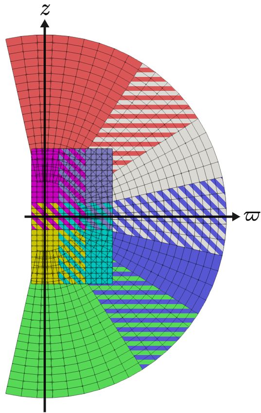
Figure 3. Percent error in the maximum density for the TOV star. Error is shown for grid
resolutions of 50 × 50, 100 × 100, and 200 × 200. The error for the 100 × 100 and 200 × 200
resolutions have been scaled up by the square of the change in resolution from the 50 × 50
case.
an EoS with nuclear physics-motivated cold component plus a simple thermal Gamma-law
component added on. In terms of baryonic number density n = ρ0 /mamu and internal energy
density u,
P (n, u) = Pc (n) + (Γth − 1)(u − uc ), (62)
where
d[Uc /n]
Pc (n) = n2 . (63)
dn
The first law gives
nT dS = −(u + P )dn + ndu. (64)
Combining the three above equations yields, after a short calculation,
nT dS = ρΓ0 th d (u − uc )ρ0 −Γth ,
(65)
so (u − uc )ρ0 −Γth advects for adiabatic change, indicating that this is an acceptable S variable.
For Gamma-law EoS, one can set uc = 0, yielding the standard auxiliary entropy variable (up
to a scaling factor) for this case.Axisymmetric Hydrodynamics in Numerical Relativity Using a Multipatch Method 17
0.000 ms 4.926 ms 14.778 ms
100 100 100
ρ (g cm−3 )
1015
z(km)
50 50 50 1013
1011
0 0 0
0 50 100 0 50 100 0 50 100
29.556 ms 44.334 ms 73.890 ms 109
100 100 100
107
z(km)
50 50 50
105
103
0 0 0
0 50 100 0 50 100 0 50 100
$(km) $(km) $(km)
Figure 4. Evolution of density profiles of the differentially rotating viscous star with mixing
length `mix = 147 m. The first panel shows the outlines of each of the overlapping subdomain
patches used to construct the computational domain.
3. Tests
3.1. TOV Star
Initial stability testing was performed using a TolmanOppenheimerVolkoff (TOV) star in a
stationary state. The star was created using a polytropic equation of state with polytropic
index Γ = 2, polytropic constant κ = 100G3 c−4 M 2 = 1.82 × 1010 cm5 g−1 s−2 , and a central
density of 7.72 × 10¹⁴ g cm−3 . This resulted in a gravitational mass of 1.38 M , a baryonic
rest mass of 1.49p M and a circumferencial radius of 14.22 km. The star was evolved for
2.46 ms = 20 R3 /(GM ) in 2D, using both axisymmetry and equatorial symmetry. The
computational domain was a square grid 14.7 km × 14.7 km in size, and was evolved using
four different resolutions with uniform grid spacing: 50 × 50, 100 × 100, and 200 × 200 grid
points. For this test, we evolve using the Cowling approximation, meaning the metric is held
fixed.
In Fig. 3 we plot the percent error in the maximum density of the star over time for each
resolution, rescaled . We see an initial spike in density at the center of the star. This is caused
by relaxation of the surface of the star, creating a disturbance that moves inward. Density
is continuous but not smooth at the surface, so this feature exhibits approximately first-order
convergence. After this initial peak settles, we see second-order convergence.Axisymmetric Hydrodynamics in Numerical Relativity Using a Multipatch Method 18
104
Ω (rad s−1 )
103.5 t = 0 ms
t = 0.4926 ms
t = 1.4778 ms
t = 7.3890 ms
t = 73.890 ms
103
100 101
$ (km)
Figure 5. Rotational velocity profile of the viscous differentially rotating star in the equatorial
plane at multiple times. We see the rotation profile begin to flatten as viscous effects
redistribute angular momentum inside the star.
3.2. Differentially Rotating Star
We choose a star with very similar profiles and global properties as the differentially rotating
star used in Shibata et al [33] and likewise use this star to test the evolution of a system under
the influence of an effective viscosity. We point out that this system is not only a useful test
of the effective viscosity code, but is designed to resemble the outcome of a binary neutron
star merger. Thus, the simulations in [33] indicate that the interior of the post-merger remnant
approaches uniform rotation on a timescale of milliseconds, with the outer layers expanding
to form a torus around the central star. Over the next ∼ 102 ms, viscous effects acting on the
outer star and torus drive an outflow of ∼ 10−2 M (for sufficiently strong viscosity). Below,
we demonstrate stable hydrodynamic evolution for 100ms, and we confirm the formation of
the envelope and massive torus structure able to give rise to outflows using an independent
code and different viscosity treatment than [33].
The star has an initial baryonic rest mass of 2.64 M and an equatorial radius Re = 10.2
km. We use a piecewise polytropic equation of state, in two pieces, of the form
(
κ1 ρΓ1 , ρ ≤ ρt
P = (66)
κ2 ρΓ2 , ρ ≥ ρt ,
where κ1 and κ2 are polytropic constants, Γ1 and Γ1 are the polytropic indices, and ρt is the
density at which we transition between the two pieces. For this star, we choose the polytropic
indices to be Γ1 = 4/3 and Γ2 = 11/4; we set the transition density between the two to beAxisymmetric Hydrodynamics in Numerical Relativity Using a Multipatch Method 19
ρt = 1.91 × 10¹⁴ g cm−3 and the low-density polytropic constant to κ1 = 0.15GM 2/3 .
The initial rotation profile for the star is given by ut uφ = Â(Ω0 − Ω) where Ω0 is the
angular velocity along the rotation axis and we choose  = 0.8Re . The initial equilibrium
state is supplied by the code of Cook, Shapiro, and Teukolsky [53].
In order to handle outflows that will occur when viscosity is enabled, we create a
computational grid better suited for resolving both the central star and low density outflowing
material. Since any outflows that occur will rapidly drop in density and are not expected to
have any small detail features of concern after they leave the region of the star, we leverage the
utility of the multipatch technique to apply differing grid structures to each zone of interest.
In the central region containing the star we employ the same rectangular grid structure as seen
in the previous TOV star test, with a resolution of 100×100 grid points. In the outflow region
we switch to a polar grid with constant latitude resolution (so that the proper spacing between
angularly adjacent points increases with distance from the star). The polar grid has 50 points
in the angular direction (covering 0 < θ < π/2) and 400 points in the radial direction. We
apply a map to the entire grid that allows us to reduce radial resolution at large distances:
R = r + 2e−γβ sinh(γr), (67)
where r is the radius in grid coordinates (the coordinates in which radial grid spacing is
uniform), and R is the radius in the original quasi-isotropic, asymptotically-Minkowski
coordinates. The map provides an approximately linear grid spacing for radii less than β,
which we have chosen to be at 25.85 km, and then switches to an exponential grid spacing
based on γ, which is chosen such that router = 73.5 km is mapped to Router = 2205 km. The
pseudospectral grid used for the evolution of Einstein’s equations is composed of an inner ball
at the center of the star surrounded by a series of spherical shells extending to a distance of
2940 km.
We impose a density floor outside of the star which is necessary to avoid division by
zero in our finite difference solver. At densities below the floor we recover temperature and
velocity using the prescription described in [54]. We recover the primitive variables from the
conservative variables using the auxiliary entropy variable in these areas using the process in
[29]. In this test, we have modified the density floor from our previous implementations to
use a floor dependent on radius:
A
ρ0 > + B, (68)
1 + R2
where we have chosen A = 1.62 × 10⁴ g cm−3 and B = 1.62 × 10⁻² g cm−3 .
For this test, we employ the viscosity treatment described in Section II. To make a
comparison with the results of the α-viscosity model used in [12], we devise a mixing length
`mix corresponding to the same kinematic viscosity as a constant α. The α-viscosity model is
generalized to differentially rotating stars in [12] by setting
αc2s
να = , (69)
Ωe
where cs is again the local sound speed and Ωe is the angular velocity of the star at the surface
on the equator. Equating this to Eq. 41, we can get an approximate relation between theAxisymmetric Hydrodynamics in Numerical Relativity Using a Multipatch Method 20
strength of a given mixing length to that of an α-viscosity parameter:
αcs
`mix = . (70)
Ωe
For the current test we set the viscous mixing length to `mix = 147 m, giving a comparable
viscous strength to α = 0.01. The timescale for viscous angular momentum transport is
approximately R2 /ν. Using Eq. 41 gives a timescale on the order of
r 2 ` −1
mix cs −1
tvisc ∼ 10 ms . (71)
10 km 147 m 0.3c
As evolution begins the star quickly begins to transport angular momentum outward
causing the rotational velocity profile to become flatter. Although the rotation profile does
flatten, we see from Fig. 5 that the profile never completely settles into a rigidly rotating state,
and retains some differential rotation. This is a feature of this viscosity method [49].
Qualitatively the outflow near the star produces the expected distribution of material
producing a short, low density burst of material as viscosity is enabled, and at later times as
more material leaves the star a disk begins to form. Other material blows farther outward,
indicating the beginnings of a viscous-driven outflow noted in [33] which we do not follow.
The density profiles in Fig. 4 are to be compared to Figure 4 in Shibata et al [33]. We note that
even the qualitative agreement we see in the density plots is nontrivial; it requires the correct
treatment of the energy equation described in Section 2.1.4. Subgrid momentum transport
is modeled in [33] via an Israel-Stewart-type formulation of the relativistic Navier-Stokes
equations, which is analytically quite different from our treatment. Our qualitative agreement
with this previous work gives confidence that its results will not prove very sensitive to details
of the momentum transport modeling.
3.3. Magnetized Disk
We evolve a standard axisymmetric MHD test problem: a magnetized torus around a Kerr
black hole. The initial conditions for this test are matched to the “fiducial model” of
McKinney and Gammie [55]. A black hole with dimensionless spin J/M 2 = 0.938 is
surrounded by a Fishbone-Moncrief torus [56] with inner edge at rBL = 6M and specific
angular momentum determined by ut uφ = 4.281. The torus has initial maximum density
ρ0 = 1 and a Γ = 4/3 equation of state. A confined poloidal seed field is introduced via
e = A0 max(ρ0 − 1, 0)dφ,
the initial vector potential 1-form A f with A0 chosen to make the
maximum ratio of magnetic to gas pressure be around 0.01. We evolve for 3000M on a
256×256 spherical-polar grid with inner radius at rBL = 1.32M and maximum radius at
60M .
The Kerr spacetime is written in in Kerr-Schild coordinates. We make the standard
change of variables for spherical-polar disk simulations:
√
r = x2 + z 2 = ex1 , (72)
1
θ = πx2 + (1 − h) sin(2πx2 ). (73)
2Axisymmetric Hydrodynamics in Numerical Relativity Using a Multipatch Method 21
ρ
100 100
20
50 10 10−1
z(km)
z(km)
0 0
10−2
−10
−50
10−3
−20
−100
10−4
0 50 100 150 200 250 0 10 20 30 40 50 60
$(km) $(km)
Figure 6. Magnetized disk with field lines at time t = 1500M , with M the mass of the
black hole (which we set equal to one). Note that the grid extends slightly to the left of the
axis because of the symmetry ghost zones. The right panel shows the region highlighted by
the white box in the left panel. Magnetic field and velocity fields are averaged over the time
1000 < t/M < 1500. The initial maximum density in the torus is chosen to be unity. Profiles
are plotted in Kerr-Schild coordinates. The longest velocity vector arrows close to the poles
far from the black hole correspond to speed very close to 1 = c.
Setting a uniform grid in x1 , x2 concentrates resolution near the black hole and on the equator.
We set h = 0.5. Finally, because r 6= rBL we compose with a final coordinate map to map the
coordinate spheres (x2 + z 2 )1/2 = C to surfaces of constant Kerr radius rBL = C. This allows
an excision inner boundary inside the horizon rBL = r+ that conforms better to the horizon
shape.
For this run, we use a position-dependent density floor ρ0 > 10−5 r−3/2 . We also increase
ρ0 and P in the magnetically-dominated region as needed to maintain b2 /ρ0 < 10 and
b2 /P < 500, which significantly improves the step size chosen by the adaptive timestepper.
We evolve both with hyperbolic divergence cleaning and vector potential evolution. For the
vector potential evolution, we use the generalized Lorentz gauge [39]. Simpler gauges, such
e = ~v · B
as the algebraic ∂t A e and advective ∂t A e = −Lv A e give the same evolution of gauge-
invariant quantities but, after a while, at a drastically reduced timestep, presumably because
the vector potential does not remain as smooth.
The vector potential evolution benefits from added explicit dissipation. We apply Kreiss-
Oliger dissipation [57] to the evolution of Ai and Φ with a coefficient of 0.001. (Our
dissipation operator is defined as a sum of fourth derivatives with respect to local coordinates
but applied to global components of the relevant evolved variables.) Without dissipation, grid-
scale ripples appear in the magnetic field atop an otherwise reasonable field structure. If the
coefficient is increased to 10−2 , the main difference is a slightly lower asymptotic speed in
the polar jets. Kreiss-Oliger dissipation is not needed for divergence cleaning runs; in fact,
it destabilizes the magnetic field evolution near the excision zone. Instead, extra dissipation
for divergence cleaning simulations is obtained by setting the maximum signal speeds in our
HLL Riemann solver for the evolution of B̃ and Ψ to the null speeds.Axisymmetric Hydrodynamics in Numerical Relativity Using a Multipatch Method 22
The qualitative expectations for this problem are well-known and are reproduced for our
runs for both types of B field evolution. Magnetic winding generates a toroidal magnetic field,
while the magnetorotational instability triggers turbulence in the disk. Matter falls into the
black hole at an average rate of about Ṁ ≈ 10−1 . The poles become magnetically dominated.
An outgoing Poynting flux can be found in this region, and gas accelerates to near the speed
of light on the poles away from the black hole. The magnetic field energy grows for the
first 1000M , then saturates, then begins to die away at a steady rate. This decrease of the
magnetic field is not physical but it is expected in any axisymmetric simulation (at least one
not enhanced by dynamo-modeling additions to the induction equation [58]) because of the
anti-dynamo theorem. Outside the region close to the poles, a mildly relativistic wind is seen.
The configuration of the system at t = 1500M is shown in figure 6.
None of this is newsworthy, although it is reassuring to confirm for the first time that
SpEC can produce magnetically-dominated jets when they are expected. For our purposes,
the main value of this test is that we can check, for a complex, astrophysically interesting
MHD problem, that our code produces no unphysical axis artifacts in any quantity we have
checked (ρ0 , v i , B i , b2 /P ). Of course, the axis actually is a special region in this problem,
which is clearly seen in the solution, but this can easily be distinguished from artifacts of the
coordinate singularity because the latter, when they appear (as they do not in this case), have
grid-spacing width. The absence of such glitches is, in fact, a nontrivial accomplishment. For
divergence cleaning evolutions without factoring of the evolution equations, grid-scale axis
artifacts in the velocity are easily seen, although they can be suppressed by using low-order
reconstruction (MC2 [59]) near the axis. For vector potential evolutions without factoring the
computation of B̃ from Ã, axis glitches become so severe that simulations crash shortly after
accretion onto the black hole begins.
Although the results are qualitatively similar, we consider the vector potential method
superior for this problem, at least with our current implementations. In divergence cleaning
methods, Ψ builds up at boundaries, particularly the excision boundary. The amount tends
to grow with time and we fear would eventually endanger the simulation. Because of it,
magnetic energy fluxes are not reliable in the inner layer of points (while in vector potential
evolutions, the inner layer shows no problems). Presumably the solution would be to improve
the treatment of the magnetic variables at boundaries.
3.4. Neutrino Radiation
3.4.1. Spherically Symmetric Collapse Profile Initial testing of the axisymmetric neutrino
code was performed by comparing the results obtained from the spherically symmetric post-
bounce supernova profile used in [44] in both 2D axisymmetry with equatorial symmetry and
in 3D using octant symmetry. In this test we evolve the moments of the neutrino distribution
function, fluid temperature, and fluid composition (the electron fraction Ye ) for a 1D profile
constructed as a spherical average of a 2D core collapse simulation 160 ms after bounce. The
velocity of the fluid is set to zero.
We perform this test in 2D on a square grid with length 300 km and a resolution ofYou can also read