BonZeb: open source, modular software tools for high resolution zebrafish tracking and analysis - Nature
←
→
Page content transcription
If your browser does not render page correctly, please read the page content below
www.nature.com/scientificreports
OPEN BonZeb: open‑source, modular
software tools for high‑resolution
zebrafish tracking and analysis
Nicholas C. Guilbeault1,2, Jordan Guerguiev1,2, Michael Martin1,2, Isabelle Tate1,2 &
Tod R. Thiele1,2*
We present BonZeb—a suite of modular Bonsai packages which allow high-resolution zebrafish
tracking with dynamic visual feedback. Bonsai is an increasingly popular software platform that is
accelerating the standardization of experimental protocols within the neurosciences due to its speed,
flexibility, and minimal programming overhead. BonZeb can be implemented into novel and existing
Bonsai workflows for online behavioral tracking and offline tracking with batch processing. We
demonstrate that BonZeb can run a variety of experimental configurations used for gaining insights
into the neural mechanisms of zebrafish behavior. BonZeb supports head-fixed closed-loop and free-
swimming virtual open-loop assays as well as multi-animal tracking, optogenetic stimulation, and
calcium imaging during behavior. The combined performance, ease of use and versatility of BonZeb
opens new experimental avenues for researchers seeking high-resolution behavioral tracking of larval
zebrafish.
The ability to precisely track animal movements is vital to the goal of relating the activity of the nervous system
to behavior. The combination of precision tracking with systems for behavioral feedback stimulus delivery can
provide valuable insights into the relationship between sensory inputs and behavioral o utputs1–3. Methods for
high-resolution behavioral tracking and dynamic sensory feedback can be combined with methods for moni-
toring or manipulating neural circuit activity to allow researchers to explore the neural circuitry underlying
sensorimotor behaviors. These assays can also increase the throughput of behavioral experiments through the
rapid and repeatable delivery of stimuli, and allow researchers to probe the sensorimotor loop by controlling
and perturbing sensory f eedback4–6.
Despite its significance, the use of behavioral feedback technology is not standard across laboratories inves-
tigating sensorimotor integration. A key challenge in developing behavioral feedback systems is synchronizing
high-throughput devices. Relatively few software implementations have succeeded in addressing this synchro-
nization problem and most rely on software configurations that require advanced levels of technical expertise.
Bonsai, an open-source visual programming language, has recently gained traction among the neuroscience
community as a powerful programming language designed for the rapid acquisition and processing of multiple
data streams7. Currently, there are no released Bonsai packages that allow for high-speed kinematic tracking of
small model organisms, such as the larval zebrafish, while providing behavior based stimulus feedback. Here,
we present BonZeb, an open-source, modular software package developed entirely in Bonsai for high-resolution
zebrafish behavioral tracking with virtual open-loop and closed-loop visual stimulation.
Results
Overview. BonZeb provides an open-source and approachable method to implement the functionalities of
extant behavioral feedback systems. Furthermore, BonZeb supplies a range of novel utilities that extend Bonsai’s
capabilities (Fig. 1). We developed packages for high-speed video acquisition, presentation of a visual stimu-
lus library, high-resolution behavioral tracking, and analysis. BonZeb inherits Bonsai’s reactive programming
framework for processing synchronous and asynchronous data streams (Fig. 2A). The reactive framework allows
users to process incoming streams of data, regardless of whether the data are coming from a finite source (e.g.
a saved video) or continuous source (e.g. streaming from a camera). There are four major classifications of
nodes—source nodes, transform nodes, sink nodes, and combinators—which generate or manipulate streams
of data called observable sequences (Fig. 2B). Figure 2B also provides a basic example of how BonZeb performs
online behavioral tracking. An online manual for BonZeb provides details for running the presented packages
1
Department of Biological Sciences, University of Toronto Scarborough, Toronto, Canada. 2Department of Cell and
Systems Biology, University of Toronto, Toronto, Canada. *email: tod.thiele@utoronto.ca
Scientific Reports | (2021) 11:8148 | https://doi.org/10.1038/s41598-021-85896-x 1
Vol.:(0123456789)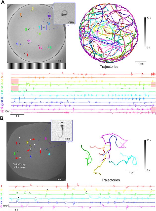
www.nature.com/scientificreports/
Figure 1. Overview of the behavioral feedback system. The behavioral feedback hardware consists of modular
components based on a previous design5. High-speed cameras convey live video of behaving larval zebrafish to
a workstation, which tracks the behavior of the fish and generates output signals to an external device to provide
sensory stimulation. The workstation processes incoming video frames with BonZeb’s customizable tracking
pipeline. This pipeline transforms behavioral data into virtual open-loop stimulation for free-swimming fish or
closed-loop stimulation for head-fixed fish. BonZeb can interface with Arduino boards, display devices, data
acquisition boards, etc., for receiving or sending data. BonZeb also includes a library of common visual stimuli
for closed-loop and open-loop visual stimulation. Components of the behavioral feedback system are not to
scale.
as well as a knowledge base for the development of new complex tracking assays (https://github.com/ncguilbeau
lt/BonZeb).
Free‑swimming behavior in virtual open‑loop. BonZeb can visually evoke and capture the core
behavioral repertoire of freely-swimming larval zebrafish using virtual open-loop assays4. To evoke predator
avoidance visual escapes, larval zebrafish were presented from below with an exponentially expanding looming
dot stimulus to either the left or right visual field at a 90° angle relative to the heading direction (Fig. 3A). Similar
to a previous s tudy8, we found that fish stimulated with a looming dot in virtual open-loop produced escape
responses characterized by a large initial turn away from the stimulus followed by high-frequency tail oscilla-
tions (Figs. 3A, 4A, Supplemental Video 1, Supplemental Video 2—700 Hz acquisition). These escape responses
were easily identified from other non-escape responses, as the max initial heading angle was consistently greater
than 50° and the max velocity exceeded 15 cm/s in all elicited escape responses (Fig. 4A, bottom left). The max
bending angle of the initial turn of the escape depended on the location of the looming stimulus such that the
initial turn consistently oriented the fish away from the stimulus (left loom escapes, n = 5, M = 100.7, SD = 27.3,
right loom escapes, n = 6, M = − 115.3, SD = 33.4, two-tailed t-test: t10 = 10.47, p < 0.001; Fig. 4A, bottom right).
Fish were stimulated to produce the optomotor response (OMR) under virtual open-loop conditions by
continually updating the orientation of a drifting black and white grating. In our open-loop OMR assay, fish
were presented with an OMR stimulus from below that was tuned to always drift in a constant direction relative
to the heading angle (90° left or right). Consistent with previous studies5, 9, we observed that fish continually
produced turns and swims to follow the direction of optic flow (Fig. 3B, Supplemental Video 3). Fish produced
significantly more clockwise turns when stimulated with rightward OMR (n = 10, M = 3.8, SD = 2.5) compared to
when stimulated with leftward OMR (n = 10, M = − 4.0, SD = 1.6, two-tailed t-test: t19 = 7.85, p < 0.001, Fig. 4B).
We also developed a novel virtual hunting assay where a small white spot is presented from below. Figure 3C
shows an example of a behavioral sequence from a fish stimulated with a virtual dot moving back and forth along
an arc of 120° positioned 5 mm away from the fish. This fish produced two J-turns when the stimulus was in a
lateral position followed by two approach swims as the stimulus moved toward the frontal field. In this example,
Scientific Reports | (2021) 11:8148 | https://doi.org/10.1038/s41598-021-85896-x 2
Vol:.(1234567890)
www.nature.com/scientificreports/

                                  Figure 2.  BonZeb inherits Bonsai’s reactive architecture for processing data streams. (A) A video source node generates images
                                  over time. The video source can either be a continuous stream of images from an online camera device or a previously acquired
                                  video with a fixed number of frames. A series of transformation nodes are then applied to the original source sequence. Each
                                  transformation node performs an operation on the upstream observable sequence that is then passed to downstream nodes. A
                                  typical pipeline consists of background subtraction, centroid calculation, tail point calculation, and finally, tail angle calculation.
                                  Nodes have a unique set of visualizers that provide the node’s output at each step. Each node has a set of properties associated with
                                  the output, such as a single coordinate, an array of coordinates, or an array of angles, which can be used for more sophisticated
                                  pipelines. (B) Bonsai workflow implementation of the above data processing pipeline. An additional node is attached at the end of
                                  the workflow to save the tail angles data to a csv file on disk. There are 4 different general classifications of nodes in Bonsai. Source
                                  nodes (green) generate new observable sequences and do not require inputs from upstream nodes. Transform nodes (blue) perform
                                  an operation on the elements of an upstream observable sequence to produce a new observable sequence that can be subscribed to
                                  by downstream nodes. Sink nodes (purple) perform side operations with the elements of the data stream, such as saving data to disk
                                  or triggering an external device. Sink nodes then pass along the upstream observable sequence to subscribed downstream nodes
                                  without modifying any of the elements of the upstream observable sequence. Combinator nodes (not shown here) are important for
                                  combining sequences and become crucial for more complex pipelines (see online manual for examples).

Scientific Reports |   (2021) 11:8148 |                    https://doi.org/10.1038/s41598-021-85896-x                                                                     3

                                                                                                                                                                    Vol.:(0123456789)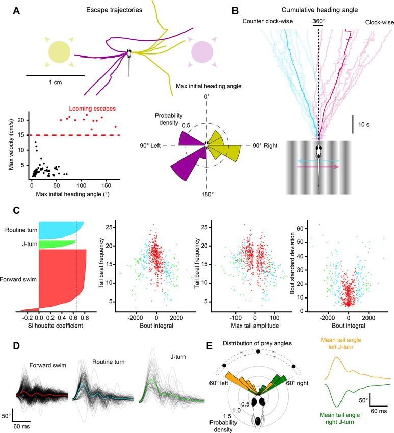
www.nature.com/scientificreports/

                                            Figure 3.  Free-swimming open-loop behavior. Individual freely-swimming zebrafish larva were presented
                                            with virtual open-loop visual stimuli while multiple behavioral metrics were recorded (332 Hz). The curvature
                                            along 14 tail segments, from the most rostral portion of the tail at the tail base to the most caudal portion of the
                                            tail at the tail tip, were calculated and averaged into 4 consecutive bins (cyan to magenta). The angle of the left
                                            (red) and right eye (green), the cumulative heading angle (yellow), the visual stimulus angle (black), tail beat
                                            frequency (orange), peak amplitudes (navy blue), and bout detection (gray) are displayed. (A) A looming dot
                                            stimulus (predator avoidance) produced a rapid escape turn followed by a burst swim and a marked divergence
                                            of the eyes (arrow). The location of the looming stimulus was fixed with respect to the heading direction and
                                            centroid position of the larvae such that the visual angle of the stimulus increased exponentially to a fixed size of
                                            the visual field. (B) During optomotor swimming, the direction of the OMR stimulus was fixed to the heading
                                            direction of the larvae and the point at which the OMR stimulus pivoted was fixed to the larva’s centroid. In
                                            this example, the OMR stimulus traversed 90° to the left of the heading direction of the fish, which consistently
                                            drove the fish to produce routine turns. (C) A small white dot on a black background was presented to larvae
                                            from below to create virtual prey stimuli. In this example, the prey stimulus moved along an arc with a fixed
                                            radius from the centroid. The velocity of the dot along the arc was defined by a sinusoidal function which
                                            reached a maximum of 100°/s directly in front of the larvae and reached a minimum of 0°/s at 60° to the left
                                            and to the right of the heading direction. Larvae displayed characteristic hunting behavior towards this stimulus
                                            by producing J-turns when the stimulus was presented to the lateral parts of the visual field and slow, approach
                                            swims when the stimulus was presented in the frontal field. These hunting episodes were also characterized by
                                            convergence of the eyes throughout the hunting episode (arrow). Images of larvae in (A–C) were adjusted so
                                            they stand out against the stimulus background.

                                            eye tracking was used to detect the characteristic eye convergence that is present in hunting larvae. Supplemen-
                                            tal Video 4 provides an example of a fish engaging in multiple hunting episodes using this stimulus paradigm.
                                            We also modified the stimulus such that the stimulus was fixed to one of the lateral extremes of the arc (60° left
                                            or right). When the prey stimulus was fixed to a lateral location in the fish’s visual field, fish often engaged in
                                            multiple J-turns with rapid succession. Supplemental Video 5 provides an example captured at a lower frame
                                            rate (168 Hz) where a fish performs 6 consecutive J-turns in pursuit of the stimulus.
                                                To determine whether virtual prey stimuli presented in the lateral visual field evoked J-turns, bouts captured
                                            during virtual prey stimulation (n = 688) were clustered based on four kinematics parameters (bout integral, max
                                            bout amplitude, mean tail beat frequency, and bout standard deviation) using hierarchical clustering (Fig. 4C). A
                                            maximum silhouette score was calculated at three clusters (silhouette score = 0.65). Three distinct clusters were
                                            detected that resembled the known kinematics of forward swims (n = 487), routine turns (n = 142), and J-turns
                                            (n = 59; Fig. 4D). We examined the location of the prey stimulus when J-turns were produced and observed that
                                            the location of the prey stimulus was not uniformly distributed, but highly skewed toward the lateral visual field
                                            (Fig. 4E). Further decomposition of the J-turn cluster into left vs right J-turns revealed that left J-turns (n = 34,
                                            Fig. 4E, top right) were produced when the prey was positioned in the far-left visual field whereas right J-turns

          Scientific Reports |   (2021) 11:8148 |                https://doi.org/10.1038/s41598-021-85896-x                                                     4

Vol:.(1234567890)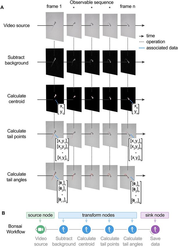
www.nature.com/scientificreports/

                                  Figure 4.  Visual stimulation drives specific behavioral kinematics. (A) Escape trajectories in the virtual open-loop
                                  looming dot assay when the looming dot was presented from the left (yellow) and from the right (magenta). Bottom left:
                                  max velocity (cm/s) with respect to the max initial heading angle (°) plotted for each bout. Bouts classified as escapes
                                  are colored red. Dashed red line represents the threshold value applied to the max velocity to select escape responses.
                                  Bottom right: probability density distribution for the max initial heading angle. (B) Cumulative heading angle over time
                                  in response to leftward (blue) and rightward (red) OMR stimulation. Spurious heading angle changes produced by fish
                                  interactions with the shallow edges of the watch glass have been removed. Rapid heading changes in the mean traces
                                  are due to the termination of shorter trials. (C) Hierarchical clustering applied to bouts in response to virtual open-loop
                                  prey stimulation. Four kinematics parameters were calculated for each bout (mean tail beat frequency, bout integral,
                                  max tail amplitude, bout standard deviation). Left: silhouette plot showing the results of hierarchical clustering with 3
                                  clusters. Dotted line represents silhouette index. Middle-left to right: kinematic parameters plotted for each bout color-
                                  coded by cluster. (D) Black lines: tail angle over time for every bout in each cluster. Colored lines represent the mean tail
                                  angle over time across all bouts in each cluster. Results from (C,D) were used to identify the three clusters as forward
                                  swims (red), routine turns (blue), and J-turns (green). (E) Bouts in the J-turn cluster were separated into left-biased and
                                  right-biased swims. Left: probability density distribution of prey yaw angles at the start of left-biased and right-biased
                                  swims in the J-turn cluster. Right: mean tail angle over time for left (yellow) and right (green) J-turns.

Scientific Reports |   (2021) 11:8148 |                  https://doi.org/10.1038/s41598-021-85896-x                                                           5

                                                                                                                                                        Vol.:(0123456789)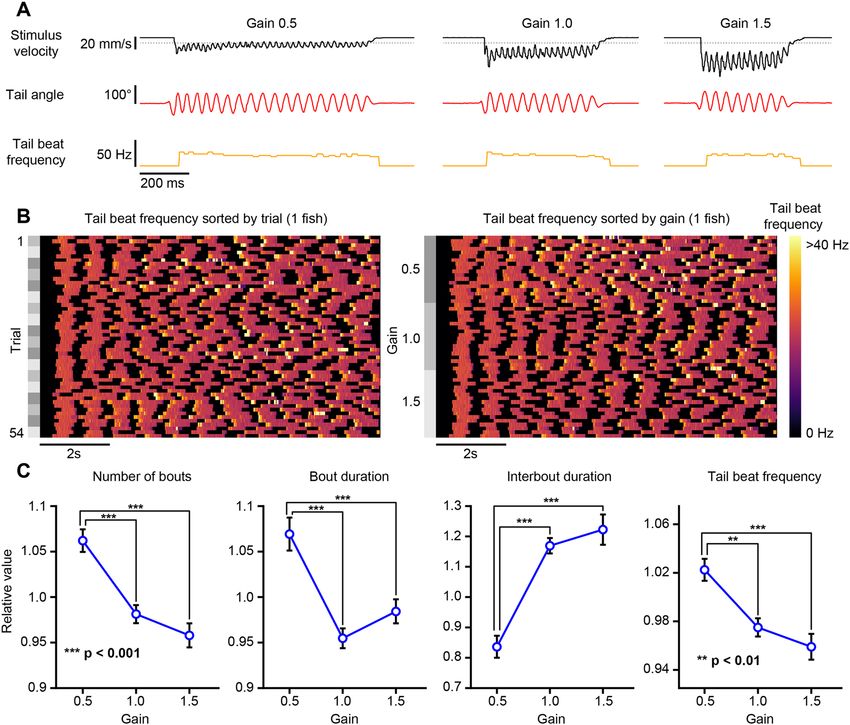
www.nature.com/scientificreports/
(n = 25, Fig. 4E, bottom right) were generated in response to prey stimuli located in the far-right visual field
(two-tailed t-test: t58 = 3.72, p < 0.001; Fig. 4E).
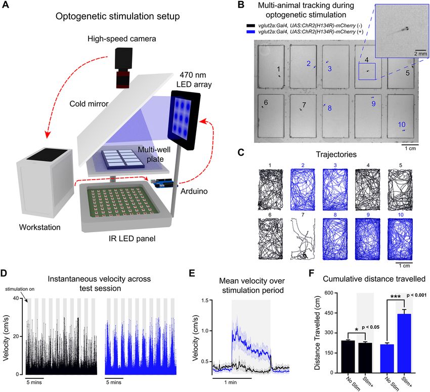
Multi‑animal tracking with visual stimulation. We created a BonZeb protocol to track multiple fish
during OMR stimulation. When the center of mass of the group crossed into the leftmost quarter of the arena,
the direction of the OMR stimulus updated to move rightwards and vice versa when the center of mass entered
the rightmost quarter of the arena. Robust optomotor swimming back and forth across the arena was observed
and real-time tracking resolved detailed tail kinematics across all individuals (n = 12); (Fig. 5A, Supplemental
Video 6 provides another example). We also developed a multi-animal hunting assay where larvae (n = 6) were
tracked while a group of moving virtual prey were projected from below. When presented with virtual prey,
larvae performed characteristic J-turns and slow approach swims (Fig. 5B).
We found that fish-to-fish contact, especially at the edges of the arena, led to sporadic swapped identities
and tracking errors. To help offset such errors, we automatically discarded regions of the dataset when larvae
physically contacted each other (Fig. 5A, red shaded regions). We calculated the percentage of tracking data
where no fish-to-fish contacts were detected and found that our method had reliably produced > 90% accuracy
with group sizes ranging from 5 to 20 (Supplemental Fig. 1C). We also sought to determine how the number of
fish tracked (centroid and tail kinematics) affected performance. The time between successive tracked frames
was normally distributed around the theoretical frame rate (3.01 ms) for a single animal tracked (M = 3.03,
SD = 0.58) and as the number of tracked fish increased, the average time between tracked frames also increased
(group size = 5, M = 3.27, SD = 1.54; group size = 10, M = 3.39, SD = 2.1; group size = 15, M = 3.55, SD = 2.25; group
size = 20, M = 3.49, SD = 2.77); (Supplemental Fig. 1B). Additionally, as the number of fish increased, we observed
a greater percentage of values in the range of 9 ms–23 ms (group size = 1, 0.08%; group size = 5, 0.91%; group
size = 10, 1.88%; group size = 15, 2.36%; group size = 20, 3.75%).
One‑dimensional closed‑loop optomotor swimming. We implemented an experimental protocol
that allowed us to present closed-loop optomotor gratings with varying feedback gain constants to head-fixed
fish. This experimental design was previously developed to investigate how optomotor swimming adapts to
altered visual feedback10. With our hardware configuration, the closed-loop round-trip stimulus delay averaged
64.1 ms with an average of 8.3 ms attributed to BonZeb processing and the remainder to stimulus delivery delays
imposed by the projector (frame buffering and refresh rate); (Supplemental Fig. 1A). Consistent with the previ-
ous study10, fish displayed stark behavioral differences between trials of different gain factors. Figure 6A shows
representative examples of bouts from the same fish under low (0.5), medium (1.0), and high (1.5) gain condi-
tions. Most notably, bouts were more frequent, longer, and had greater tail beat frequency with low gain condi-
tions compared to medium and high gain conditions (Fig. 6B,C, Supplemental Video 7). We found that fish pro-
duced a greater number of swim bouts in low gain, with bout numbers decreasing as the gain increased (n = 16,
one-way ANOVA: F2,45 = 20.76, p < 0.001; Fig. 6C, far-left). Bout duration decreased as gain factor increased
(n = 16, one-way ANOVA: F2,45 = 16.92, p < 0.001; Fig. 6C, middle left). Fish displayed shorter inter-bout inter-
vals in low gain compared to medium and high gain conditions (n = 16, one-way ANOVA: F2,45 = 29.5, p < 0.001;
Fig. 6C, middle right) and mean tail beat frequency decreased with increasing gain values (n = 16, one-way
ANOVA: F2,45 = 13.09, p < 0.001; Fig. 6C, far-right).
Multi‑animal two‑dimensional closed‑loop optomotor swimming. We designed a two-dimen-
sional closed-loop assay which provided both forward–backward, as well as angular visual feedback to multi-
ple head-fixed fish independently. This assay was inspired by a previous implementation of a two-dimensional
closed-loop optomotor assay11. We found that fish consistently responded to gratings of different orientations by
swimming in the direction of optic flow (Fig. 7A). The orientation of the gratings converged towards the head-
ing angle as trials progressed over 30 s (Fig. 7B). The probability that the final stimulus orientation converged
(P = 0.62) towards the heading angle was much greater than the probability that the orientation diverged (P = 0.28)
or remained unchanged (P = 0.11). At larger orientations, fish tended to produce turns over forward swims, as
indicated by the mean tail angle across swimming bouts. Bouts tended to transition from asymmetric turns in
the direction of the stimulus orientation to symmetric forward swims as trials progressed and the orientation
of the stimulus neared alignment with the heading angle (n = 4668, one-way ANOVA: F6,4661 = 224.01, p < 0.001;
Fig. 7C, left). The mean angular velocity of the stimulus showed a similar trend, albeit in the opposite direction,
such that the angular velocity produced by swimming bouts at large stimulus orientations was larger and tended
to align the stimulus orientation to the heading direction (n = 4668, one-way ANOVA: F6,4661 = 260.34, p < 0.001;
Fig. 7C, right). Tail beat frequency was significantly different for stimulus orientations between − 22.5° and 22.5°
compared to all other stimulus orientations. Tail beat frequency increased as the orientation of the stimulus
became aligned to the heading direction (n = 4668, one-way ANOVA: F6,4661 = 38.7, p < 0.001; Fig. 7C, middle).
Multi‑animal tracking with optogenetic stimulation. To demonstrate how BonZeb can be used for
high-throughput behavioral analysis with neural circuit manipulations, we developed a novel multi-animal
optogenetic stimulation assay (Fig. 8A). The setup allowed us to deliver stimulation to multiple fish simultane-
ously and track each fish’s trajectory over time (Fig. 8B,C). Experimental animals that expressed channelrhodo-
sin-2 in glutamatergic neurons displayed a marked increase in locomotor activity during periods of optogenetic
stimulation compared to control animals (Fig. 8D). We averaged across 2-min periods within an experiment,
starting 30 s before and ending 30 s after each stimulation period, and found the mean instantaneous velocity
of experimental animals to be greater than control animals during stimulation (Fig. 8E). We examined the total
distance travelled when stimulation was ON compared to when stimulation was OFF across the entire experi-
Scientific Reports | (2021) 11:8148 | https://doi.org/10.1038/s41598-021-85896-x 6
Vol:.(1234567890)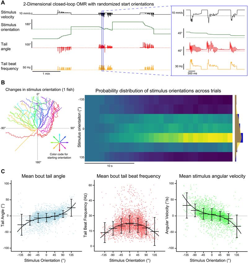
www.nature.com/scientificreports/

                                  Figure 5.  Multi-animal tracking during OMR and prey capture. (A) The position and tail curvature of 12 larvae
                                  tracked (332 Hz) during the presentation of an OMR stimulus. The direction of the OMR stimulus changed to
                                  traverse leftward or rightward depending on whether the center of mass of the group crossed into the rightmost
                                  quarter or leftmost quarter of the arena, respectively. Trajectories are individually color coded by fish and
                                  shaded by time. The tail curvature for each fish is represented as the average of the 3 most caudal tail segments.
                                  Post processing of the tail curvature data revealed sections of the data when fish physically contacted each other
                                  (red highlighted regions). The tail tracking results surrounding these encounters decreased in accuracy and
                                  occasionally produced tracking errors (arrow). (B) Freely swimming larvae in a group of 6 were tracked and
                                  presented with multi-prey stimuli projected from below. Virtual prey were programmed to produce paramecia-
                                  like behavior, defined as periods of forward movement, brief pauses, and changes in orientation. The linear
                                  velocity, distance, length of pause, angular velocity, and orientation were varied for each virtual prey. Larvae
                                  produced distinct J-turns in response to virtual prey (* = manually identified J-turn).

                                  ment for both experimental (n = 15) and control animals (n = 15). Using a mixed ANOVA, we found a significant
                                  effect for group (F1,28 = 27.42, p < 0.001), a significant effect for stimulation (F1,28 = 33.66, p < 0.001), and a sig-
                                  nificant interaction between group and stimulation (F1,28 = 45.84, p < 0.001). Pairwise comparisons using paired
                                  t-tests revealed that for the experimental animals, the total distance travelled for stimulation ON (M = 442.85,

Scientific Reports |   (2021) 11:8148 |                 https://doi.org/10.1038/s41598-021-85896-x                                                      7

                                                                                                                                                   Vol.:(0123456789)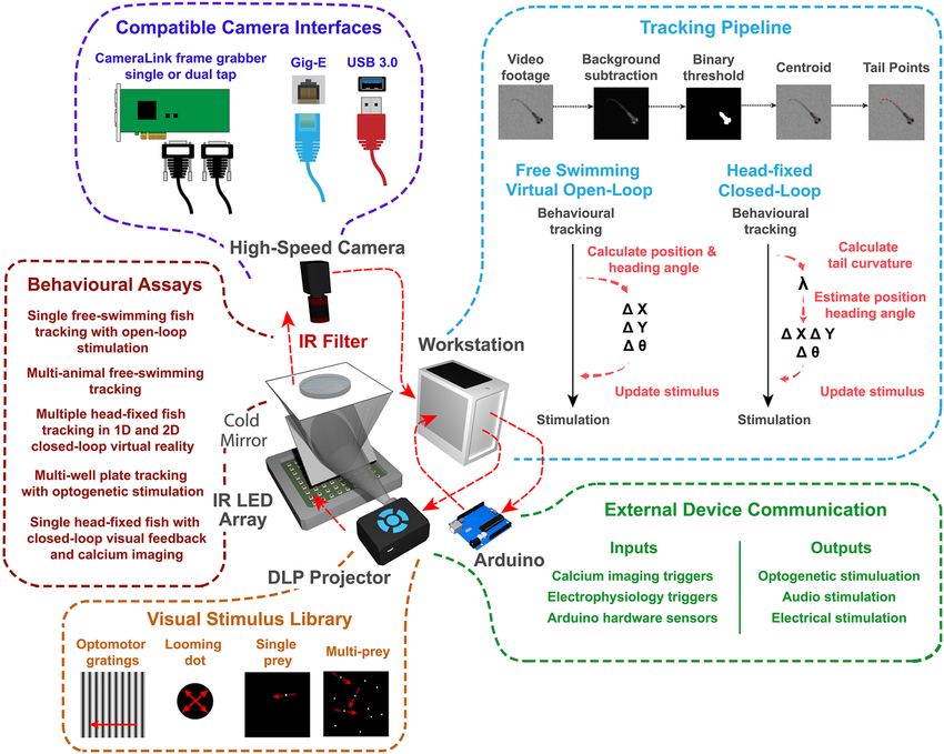
www.nature.com/scientificreports/
Figure 6. One-dimensional head-fixed closed-loop OMR. The tail of a head-fixed fish was tracked (332 Hz)
while presenting a closed-loop OMR stimulus with varying feedback gain values. (A) Example bouts taken
for each gain value for a single fish. Fish were tested on 3 different gain values. Left: gain 0.5. Middle: gain 1.0.
Right: gain 1.5. The stimulus velocity (black), tail angle (red), and tail beat frequency (orange) were recorded
continuously throughout the experiment. The stimulus velocity changed in proportion to the swim vigor
multiplied by the gain factor. Dotted lines indicate baseline value of 0. (B) An example of a single fish showing
the tail beat frequency across trials. Left: tail beat frequency sorted by trial number. Right: same data as left with
tail beat frequency sorted by gain. (C) Bout kinematics plotted as a function of gain factor.
SD = 127.31) was significantly higher compared to stimulation OFF (M = 214.73, SD = 43.53; t14 = 6.44, p < 0.001),
whereas the total distance travelled for the control animals during stimulation ON (M = 225.78, SD = 32.36) was
significantly less than stimulation OFF (M = 243.37, SD = 21, t14 = 2.2, p = 0.045; Fig. 8F).
Closed‑loop visual stimulation during calcium imaging. To demonstrate how BonZeb can be used
in combination with techniques for imaging neural activity, we implemented a one-dimensional closed-loop
OMR assay during two-photon calcium imaging. We performed volumetric calcium imaging in the hindbrain
(500 × 500 × 63 µm) of a fish expressing GCaMP6f throughout the brain during OMR s timulation12. We imaged
at 2.7 Hz using an objective piezo and resonant scanning (9 z-planes, 7 µm spacing). OMR stimulation was pre-
sented to one side of the fish using a projector (Fig. 9A). We found that fish consistently produced swims when
forward moving gratings were presented (Fig. 9B). We used an automated ROI extraction method, based on the
CaImAn analysis p ackage13, to find 25 neuronal ROIs in the hindbrain for each imaged z-plane (Fig. 9C). We
observed an increase in neuronal activity across planes during swim bouts, in agreement with previous studies
where hindbrain activity was shown to be highly correlated with swimming5, 14, 15 (Fig. 9D).
Discussion
Behavioral tracking systems for larval zebrafish have previously been developed using both commercial and open-
source programming languages. ZebraZoom, written in MATLAB, provides methods for high-speed tracking and
behavioral classification16. Additionally, the open-source Python program Stytra performs high-speed open-loop
and closed-loop tracking of larval zebrafish17. BonZeb provides a unique tracking solution for zebrafish in that
Scientific Reports | (2021) 11:8148 | https://doi.org/10.1038/s41598-021-85896-x 8
Vol:.(1234567890)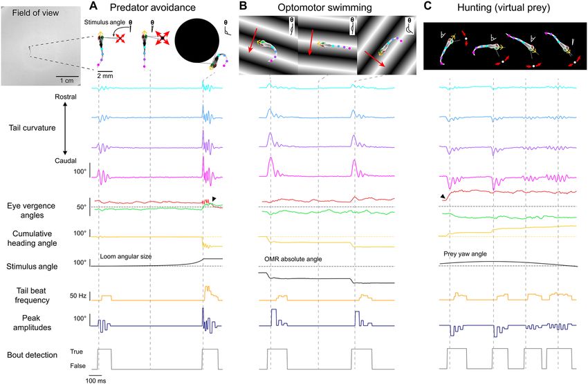
www.nature.com/scientificreports/
Figure 7. Multi-animal two-dimensional closed-loop OMR. The tails of four head-fixed fish were tracked
(332 Hz) while each fish was presented with a two-dimensional closed-loop OMR stimulus. (A) Data collected for
each fish included the stimulus velocity (black), stimulus orientation (green), tail angle (red) and tail beat frequency
(orange). The stimulus velocity changed in proportion to the tail beat frequency and current stimulus orientation.
The stimulus orientation changed with the tail angle. Trials were 30 s long and were preceded by a 1-min rest
period where only the stimulus velocity and stimulus orientation data were recorded. At the end of each trial, the
orientation of the stimulus was reset to one of the 8 randomized start orientations. (B) Stimulus orientation over
time. Left radial plot: stimulus orientation is plotted for all trials for a single fish. Trials are color-coded based on
initial starting orientation and extend outwards from the origin as a function of time. Right heatmap: normalized
histograms of stimulus orientations over time across fish (n = 16). Binning was 1 s for the x-axis and 45° for the
y-axis. Far right plot: histogram and kernel density estimate of the distribution of orientations at the end of trials
across all fish. (C) Bout kinematics and stimulus angular velocity are plotted for each bout as a function of stimulus
orientation at bout onset. Orientations were divided into 45° bins and the median and standard deviation for each
bin are plotted. A polynomial function was fit to each dataset. The mean bout tail angle and mean stimulus angular
velocity were fit with 3rd degree polynomials (R2 = 0.223 and R2 = 0.256, respectively) whereas the mean bout tail
beat frequency was fit with a 2nd degree polynomial ( R2 = 0.05).
Scientific Reports | (2021) 11:8148 | https://doi.org/10.1038/s41598-021-85896-x 9
Vol.:(0123456789)www.nature.com/scientificreports/
Figure 8. Free-swimming multi-animal tracking during optogenetic stimulation. Ten larvae were tracked
simultaneously (200 Hz) in a multi-well plate while being subjected to epochs of optogenetic stimulation. (A)
3D schematic of the optogenetic stimulation setup. Live video is processed by BonZeb, which sends commands
to an Arduino to generate a digital signal for triggering a 470 nm LED array (0.9 mW/mm2 at the plate).
Components of the optogenetic setup are not to scale. (B) Example of a single video frame. Data are color coded
based on genetic background. (C) Example of trajectories over an entire 20-min test session. (D) Instantaneous
velocities for all fish plotted across the entire test session. Shaded regions represent periods when optogenetic
stimulation occurred. 1-min intervals of stimulation and no stimulation repeated throughout the assay with
a 30 s no stimulation period occurring at the beginning and end of the assay. Left: instantaneous velocity of
control larvae (n = 15). Right: instantaneous velocity of experimental larvae (n = 15). (E) Mean instantaneous
velocity averaged across all fish and all stimulation periods. Instantaneous velocity across each stimulation
period was averaged for each fish and convolved with a box car filter over a 1s window. Bold line represents the
mean and shaded region represents SEM. (F) Cumulative distance travelled during periods of stimulation ON
(Stim +) and stimulation OFF (No stim).
it inherits Bonsai’s framework, uses a high-performance compiled programming language (C#), and operates
through a visual programming interface. BonZeb also provides a suite of fully developed visuomotor assays that
cover many existing needs for zebrafish researchers.
We demonstrate that BonZeb can perform high-speed online tracking during virtual open-loop predator
avoidance, OMR, and prey capture assays. Larvae produced characteristic J-turns, slow approach swims, and eye
convergence in response to a small prey-like stimulus in virtual open-loop, consistent with previous findings from
naturalistic and virtual prey capture s tudies18–20. In response to optomotor gratings, larvae continually produced
turns in the direction of the stimulus, similar to what has been described p reviously5, 9. In our predator avoidance
assay, larvae displayed rapid directional escape behavior when looming stimuli were presented to either side of
the fish in agreement with prior r esults8, 21. In the multi-animal OMR assay, we used group behavior to control
the direction of optic flow while performing simultaneous online tail tracking for each fish. In the multi-animal
Scientific Reports | (2021) 11:8148 | https://doi.org/10.1038/s41598-021-85896-x 10
Vol:.(1234567890)www.nature.com/scientificreports/
Figure 9. Calcium imaging during closed-loop OMR. One-dimensional closed-loop optomotor gratings were
presented to a head-fixed larva while simultaneously performing fast volumetric two-photon calcium imaging.
(A) Single frame obtained from the behavior camera showing the larva’s tail with the OMR stimulus represented
(stimulus spatial frequency was lower than depicted; 450 Hz tracking). The OMR stimulus was presented from
the side and travelled from caudal to rostral. (B) Tail angle and stimulus velocity across the entire 1-min trial.
Movement of the closed-loop OMR stimulus began at 15 s and continued for 30 s. (C) Maximum intensity
z-projection overlaid with neuronal ROIs found in the medial hindbrain. 25 ROIs were selected for each z-plane
and color-coded by depth. Automated ROI extraction was performed throughout the region enclosed in dotted
red line which helped minimize the detection of non-somatic ROIs. (D) Z-scored ROI responses across the trial.
prey capture experiment, numerous virtual prey stimuli, presented from below, elicited J-turns toward prey
targets across all individuals. As expected, fish displayed much tighter swimming trajectories in the prey assay
compared to the long swimming trajectories fish produced in the OMR assay.
The head-fixed assays we developed for BonZeb allow for closed-loop optomotor stimulation in one or
two dimensions. In our one-dimensional closed-loop assay, we found that fish produced more bouts more
frequently under low gain conditions, with individual bouts having longer durations and higher tail beat fre-
quency compared to bouts generated in high gain conditions. These results agree with previous research that
also investigated the effect of visual reafference mismatching on optomotor swimming10, 14. Our method for
head-fixed two-dimensional closed-loop visual feedback builds on the methods of previous research to provide
two-dimensional, closed-loop visual feedback to multiple animals simultaneously11, 22. When presented with
randomized initial starting orientations, larvae consistently responded to the OMR stimulus by swimming in
the direction of optic flow. Swim bouts were found to align the stimulus orientation toward the animal’s heading
direction, in agreement with previous results11. We also found that larvae increased their tail beat frequency as
the stimulus orientation neared the heading angle.
Bonsai provides a convenient framework for BonZeb to integrate with external devices. We demonstrate this
feature with a novel optogenetics assay as well as closed-loop OMR stimulation during calcium imaging. BonZeb’s
flexibility in creating tracking pipelines and support of hardware integration allows new users to rapidly develop
and implement complex behavioral assays. An exciting future direction is the incorporation of BonZeb’s video
acquisition, behavioral tracking, and stimulation capabilities with more complicated 3D visual rendering pipe-
lines using the recently developed BonVision package. This combination would allow the creation of complex
immersive environments for virtual open and closed-loop approaches23. In summary, BonZeb provides users
Scientific Reports | (2021) 11:8148 | https://doi.org/10.1038/s41598-021-85896-x 11
Vol.:(0123456789)www.nature.com/scientificreports/
with a suite of fast, adaptable and intuitive software packages for high-resolution larval zebrafish tracking and
provides a diverse set of visuomotor assays to investigate the neural basis of zebrafish behavior.
Methods
BonZeb installation and setup. A detailed manual for installation, setup and programming in BonZeb
can be found on GitHub (https://github.com/ncguilbeault/BonZeb). Briefly, users will need to download and
install Bonsai (https://bonsai-rx.org/docs/installation) and the packages required to run BonZeb workflows.
Bonsai Video and Bonsai Vision packages are used for video acquisition and video analysis, Bonsai Shaders is
used for OpenGL graphics rendering, and Bonsai Arduino is used for communication with Arduino microcon-
trollers. Packages for BonZeb can be downloaded from Bonsai’s built-in package manager.
Video acquisition. BonZeb can be used with a variety of cameras already supported by Bonsai. The Fly-
Capture package integrates FLIR cameras and the PylonCapture package integrates Basler cameras. As well,
the Bonsai Vision package offers access to DirectShow driver-based cameras, such as USB webcams. We have
developed packages to incorporate Allied Vision Technologies (AVT) USB 3.0 cameras, Teledyne DALSA GigE
cameras, and CameraLink cameras that use Euresys frame grabber boards. Bonsai uses OpenCV for video acqui-
sition and video processing. Thus, our packages use the same implementation of OpenCV structures, formats,
and data types. These packages are written in the native C#/.NET language underlying Bonsai’s framework. Our
Allied Vision, Teledyne DALSA, and Euresys packages utilize the software development kits (SDK) and .NET
libraries (DLLs) provided by the manufacturers to acquire, process, and display frames in Bonsai. Each of our
video capture packages offers unique properties for controlling the connected camera’s features. For example,
the VimbaCapture module from the Allied Vision package allows users to control features of an AVT camera
such as frame rate, exposure, black level, gain, and gamma. The output is a VimbaDataFrame, containing
the image, a timestamp, and a frame ID associated with each image. Similarly, the SaperaCapture module
performs the same control and output functions for Teledyne DALSA GigE cameras. The properties of each
module can be changed dynamically. The ability to modify the camera’s specific features on the fly enables users
to quickly optimize the camera’s acquisition properties with respect to their specific imaging requirements. The
MultiCamFrameGrabber module from the Euresys Frame Grabber package allows users to specify prop-
erties such as the ConnectionType, BoardTopology, and CameraFile. While this module does not
support dynamic changes to the specific camera’s acquisition features, users can modify the camera file for their
camera prior to running Bonsai to adjust the camera’s acquisition settings. The MultiCamFrameGrabber
module should be compatible with any CameraLink camera that is supported by a Euresys frame grabber board.
Behavioral tracking. BonZeb’s package for behavioral tracking is written in C#/.NET and utilizes OpenCV
data types for efficient image processing and analysis. We built a CalculateBackground module that com-
putes the background as the darkest or lightest image over time (Algorithm 1). This operation works by compar-
ing each individual pixel value of the gray scale input image with the pixel values of a background image con-
tained in memory. The module updates the internal background image only if the pixel value of the input image
is greater than the corresponding pixel value of the background image. In this way, if the subject for tracking
is darker than the background and the subject has moved, the output of the CalculateBackground node
will consist of a background image that has successfully removed the subject. By changing the PixelSearch
property, users can set the module to maintain either the darkest or lightest pixel values in the input image. The
optional NoiseThreshold parameter can be set to modify the background calculation such that the pixel
value of the input image must be greater than or less than the pixel value of the background and some additional
noise value. This background calculation method offers advantages over Bonsai’s pre-existing methods for back-
ground calculation because it enables rapid background subtraction and only requires a small amount of move-
ment from the animal to obtain a reliable background image.
Scientific Reports | (2021) 11:8148 | https://doi.org/10.1038/s41598-021-85896-x 12
Vol:.(1234567890)www.nature.com/scientificreports/
We also provide a module for performing efficient centroid calculation using the CalculateCentroid
module. This module takes an image as input (usually represented as the background subtracted image) and
finds an animal’s centroid using the raw image moments or by finding the largest binary region following a binary
region analysis. The method for centroid calculation is set by the CentroidTrackingMethod property.
The ThresholdValue and ThresholdType properties set the value of the pixel threshold and the type of
threshold applied (binary threshold or inverted binary threshold). If RawImageMoments is used, Calcu-
lateCentroid calculates the centroid using the center of mass of the entire binary thresholded image. The
LargestBinaryRegion method performs a contour analysis on the thresholded image to find the contour
with the largest overall area. This method utilizes the MinArea and MaxArea properties to discard contours
whose area lies outside of the defined range. The result of the CalculateCentroid operation using the
largest binary region method is the centroid of the contour whose area is the largest within the allowed range of
possible areas. In most experiments, the LargestBinaryRegion method will be more robust against image
noise than the RawImageMoments method.
The centroid and the image can then be combined and passed onto the CalculateTailPoints mod-
ule, which fits points along the tail using an iterative point-to-point contrast detection algorithm seeded by the
centroid. Two pre-defined arrays are calculated containing the points along the circumference of a circle with
a given radius centered around the origin. The first array consists of points along a circle whose radius is equal
to the DistTailBase property. When the HeadingDirection property is negative, the most rostral tail
point is found by searching the first array, whose points have been shifted such that the origin is at the centroid.
If the HeadingDirection is positive, the first tail point is taken as the point in the array whose angle from
the centroid corresponds to the angle in the opposite direction provided by the HeadingDirection. For
Scientific Reports | (2021) 11:8148 | https://doi.org/10.1038/s41598-021-85896-x 13
Vol.:(0123456789)www.nature.com/scientificreports/
subsequent tail points, a second array is used that contains points along the circumference of a circle with a
radius equal to the DistTailPoints property. A subset of points in this array are calculated and searched
for subsequent tail points. This subset of points corresponds to an arc with length determined by the Rang-
eTailPointAngles property. The midpoint of the arch is determined by the point in the array where the
angle is closest to the angle calculated between the previous two tail points.
Three different contrast-based point detection algorithms can be selected for calculating tail points in the
CalculateTailPoints module specified by the TailPointCalculationMethod property. The
PixelSearch option is the simplest of the three algorithms and works by taking the darkest or lightest pixel
within the array of points. The WeightedMedian method involves taking the median of the points whose
pixel values are weighted by the difference from the darkest or lightest pixel value. The CenterOfMass method
calculates the center of mass using the difference of each pixel value from the darkest or lightest pixel value and
taking the point in the array that is closest to the center of mass. All three algorithms can calculate the corre-
sponding tail points of the fish efficiently, however, differences between each algorithm will make one or another
more desirable depending on the specific needs of the application. While the PixelSearch method is faster
than the other two methods, the calculated tail points tend to fluctuate more between successive frames. The
WeightedMedian and CenterOfMass methods tend to reduce the amount of frame-to-frame fluctuations
but take longer to compute. Despite the minor differences in computational speed, all three algorithms can reli-
ably process images with 1 MP resolution acquired at 332 Hz. Changing the PixelSearchMethod property
of the CalculateTailPoints function will determine whether the algorithm searches for the lightest or
darkest pixel values in the image. How many tail points are included in the output depends on the value given to
the NumTailSegments property, such that the number of points in the output array is the NumTailSeg-
ments value plus 2. The array is ordered along the rostral-caudal axis, from the centroid to the tip of the tail.
Lastly, the CalculateTailPoints function contains the optional OffsetX and OffsetY properties which
allows users to offset the final x and y coordinates of the calculated tail points.
The output of the CalculateTailPoints is used to extract information about the tail curvature using
the CalculateTailCurvature module. This function converts an array of points along the tail, P = [(x0,
y0), …, (xn, yn)] (ordered from the most rostral to the most caudal), into an array of values Θ = [θ1, …, θn]. The
values in the output array correspond to the angles between successive points in the input array normalized to
the heading direction. The heading direction (θh) is given as the angle between the second point in the array (the
most rostral tail point) and the first point (the centroid):
θh = −atan2 y1 − y0 , x1 − x0
where (xi, yi) is the ith point along the tail and atan2 is an inverse tangent function that constrains θh such
that −π < θh ≤ π. Each point in the array is translated by an amount that is equivalent to translating the centroid
to the origin. The heading angle is used to rotate each point in the translated array such that the first angle in
the output array is always 0:
xi∗ = (xi − x0 ) cos θh − yi − y0
sin θh
yi∗ = (xi − x0 ) sin θh + yi −
y0 cos θh
θi = atan2 yi∗ − y0 , xi∗ − x0 for i ∈ [1, . . . , n]
The length of the output array is equivalent to the length of the input array (number of tail points) minus 1.
One final computation is performed to normalize the angles. This involves iterating through the entire array and
offsetting an angle in the array by 2π if the absolute difference between the current angle and the previous angle
is greater than π. This ensures that the angles across all tail segments are continuous and removes disparities
between successive angles when relative angles change from − π to π.
The output of the CalculateTailCurvature module can then be passed onto the DetectTail-
BeatKinematics module which outputs a TailKinematics data structure containing peak amplitude,
tail beat frequency, and bout instance. The algorithm used by the DetectTailBeatKinematics module
(Algorithm 2) works by comparing the current tail angle to an internal memory of the minimum and maximum
tail angle over a running window. The difference between the current tail angle and either the maximum or
minimum tail angle is used to compare the current tail angle to a threshold, specified by the BoutThreshold
property.
If the difference exceeds this threshold, then the algorithm sets the bout detected value to true and begins
searching for inflection points in the stream of input data. The time window, specified by the FrameWindow
property, determines how many tail angle values to maintain in memory and how many times the counter vari-
able, initialized at the start of a bout and incremented by 1 for each frame a bout is detected, should increment
while continuing to search for successive points in the input stream. When a bout is detected, if the difference
between the current tail curvature and the maximum or minimum value is less than or greater than the threshold
value set by the PeakThreshold, then the algorithm begins searching for inflection points in the opposite
direction and the peak amplitude is set to the maximum or minimum value. If more than one inflection point
has been detected within a single bout, then the tail beat frequency is calculated by dividing the FrameR-
ate property by the number of frames between successive peaks in the input data. When the counter variable
exceeds the specified FrameWindow, the counter variable resets, the bout instance is set to false, and the peak
amplitudes and tail beat frequency are set to 0.
Scientific Reports | (2021) 11:8148 | https://doi.org/10.1038/s41598-021-85896-x 14
Vol:.(1234567890)www.nature.com/scientificreports/
The output of the CalculateTailPoints function can be used to find the coordinates of the eyes using
the FindEyeContours module. The FindEyeContours module takes a combination of the array of tail
points and a binary image. It processes the image using the output of the CalculateTailPoints function
to calculate the binary regions corresponding to the eyes. To maintain consistency across our package and the
Bonsai Vision package, the output of the FindEyeContours module is a ConnectedComponentCol-
lection, the same output type as the BinaryRegionAnalysis module, which consists of a collection
of non-contacting binary regions called “connected components”. The algorithm for finding the eyes starts by
performing a contour analysis on the input image, the parameters of which can be specified using the Mode
and Method properties to optimize the contour retrieval and contour approximation methods, respectively.
Once all of the contours in the image are acquired, contours whose area lie outside the range of areas provided
by the MinArea and MaxArea properties and whose distance from the centroid of the tracking points lies
outside the range of distances given by the MinDistance and MaxDistance properties, are discarded from
further analysis. The remaining contours are then ordered by centering their position around the centroid of the
tail tracking points, rotating each contour to face forward with respect to the heading angle, and calculating the
absolute difference between the heading angle and the angle between the centroid and the contours’ centroid.
The array of contours is ordered in ascending order with respect to the difference between the angle to the
centroid and the heading angle. The algorithm continues to discard regions that do not correspond to the eyes
by discarding regions that lie outside the AngleRangeForEyeSearch property, which is centered around
the heading angle. The contours are then ordered by their angles once more, such that the final Connected-
ComponentCollection consists of the left eye and right eye, respectively. The algorithm also provides the
additional FitEllipsesToEyes property to allow users to fit ellipses to the eyes.
The output of the FindEyeContours module can be combined with the output of the Calculate-
TailPoints function and provided as input to the CalculateEyeAngles function to calculate the con-
vergence angles of the left and right eye with respect to the heading angle. For each eye, the function calculates
the point p = (x, y) whose distance from the origin is equal to the length of the binary region’s major axis, lM, and
whose angle from the origin corresponds to the orientation of the major axis, θM:
Scientific Reports | (2021) 11:8148 | https://doi.org/10.1038/s41598-021-85896-x 15
Vol.:(0123456789)www.nature.com/scientificreports/
x = lM cos θM
y = lM sin θM
The point is then rotated with respect to the heading angle and the new angle between the point and the
origin, θ * , is calculated:
x ∗ = x cos θh − y sin θh
y ∗ = x sin θ h + y cos
θh
θ∗ = atan2 y ∗ , x ∗
The orientation of the binary region’s major axis orientation is always between 0 and π. This poses a problem
for calculating the orientation of the eyes with respect to the heading direction, which is between 0 and 2π,
because the orientation of the eyes needs to be in a consistent direction with respect to the heading angle. The
CalculateEyeAngles module accounts for this by checking which direction the angle of the eye faces
with respect to the heading direction and then offsets the angle by π if the eye angle is initially calculated in the
opposite direction. Alternatively, the heading angle, derived from the CalculateHeadingAngle module,
can be substituted for the array of tail points as input into the CalculateEyeAngles function to determine
the angles of the eyes with respect to the heading angle if only the centroid and heading angle data are available.
A combination of the array of tail points, generated by the CalculateTailPoints operation, and the eye
contours, generated by the FindEyeContours function, can be passed as input to the CalculateHead-
ingAngle module to calculate a more accurate representation of the heading angle using the angle between the
centroid and the midpoint between the centroids of the two eyes. The CalculateHeadingAngle module,
which tracks the cumulative heading angle over time, also has an option to initialize the heading angle to 0 at the
start of recording, which can be set with the InitializeHeadingAngleToZero property.
Visual stimulus library. We used the Bonsai Shader package and OpenGL to compile a library of vis-
ual stimuli that can be used for closed-loop and virtual open-loop assays. Virtual open-loop visual stimuli are
updated based on the position and heading direction of the animal. The library contains the following stimuli:
looming dot, optomotor gratings, phototaxic stimuli, optokinetic gratings, single or multiple prey-like small
dots, and whole field luminance changes (black and white flashes). Additionally, we have developed a method
for closed-loop stimulation of head-restrained animals using methods we have developed for analyzing the tail
curvature of head-restrained larval zebrafish to estimate changes in position and heading direction. We demon-
strate how to use this method to provide head-fixed larval zebrafish with one-dimensional or two-dimensional
closed-loop OMR stimulation. Our method for closed-loop OMR stimulation in head-fixed animals can be eas-
ily extended to work with other stimuli such as the looming dot stimulus, prey stimulus, and multi prey stimulus.
Calibrating the display device to the camera involves identifying the areas of the display that correspond to
the camera’s field of view (FOV). To do so, users need to align the edges of a projected box onto the edges of
the camera’s FOV. Users can either remove the IR filter on the camera to allow the image from the display to
show up on the camera, or use an object, such as a translucent ruler, as a common reference to align the edges
of the projected box to the edges of the camera’s FOV. We developed a fast and reliable method to map this area
using the DrawRectangle module, which allows users to draw a rectangle onto an input image and outputs
a CalibrationParameters construct. The outputs of the CalibrationParameters can then be
mapped directly onto a stimulus to modify the area the stimulus is presented to. By drawing a simple rectangle
shader onto a specific area of the display, the user can then determine the area of the projector that corresponds
to the camera’s FOV.
Virtual open‑loop and closed‑loop setup. We implemented an established optomechanical configu-
ration to record behavior of fish and project computer generated stimuli from b elow5, 8, 9. This setup included
a projector for visual stimulation, an infrared backlight for fish illumination, a cold mirror and a high-speed
camera equipped with a long-pass filter. A Sentech STC-CMB200PCL CameraLink camera (Aegis Electronic
Group, Inc.) was used. The camera was integrated using a GrabLink Full XR Frame Grabber (Euresys Inc.). This
configuration allowed us to acquire 1088 × 1088 resolution frames at 332 Hz. We also used the same configura-
tion to acquire 640 × 480 resolution frames at 700 Hz. We used a fixed focal length (30 mm) lens (Schneider-
Kreuznach) equipped with a long-pass filter (Edmund Optics) to block out the visible light from back-projected
stimuli presented from below the camera. A high-definition, 1920 × 1080, 60 Hz, DLP pico projector (P7, AAXA
Technologies Inc.) was used for visual stimulation and a 25 × 20 cm cold mirror (Knight Optical) reflected vis-
ible light from the projector upwards to the bottom of the platform. An 850 nm LED array (Smart Vision Lights)
provided tracking light and was placed underneath the cold mirror. The platform consisted of a 6 mm thick
transparent polycarbonate sheet (20 cm × 22 cm), with mylar diffusion paper placed on top for back projection.
The workstation computer was equipped with an Intel Core i9-9900 K processor, an ASUS ROG GeForce GTX
1060 graphics card, and 64 GB of RAM.
Virtual open‑loop looming stimulation. Fish were placed in a 6 cm watch glass inside a 10 cm petri
dish. Both the petri dish and watch glass were filled with filtered system. The water was 5 mm in depth. Looming
stimulation trials were 20 s long. The angular size to speed ratio (l/v) of the looming stimulus was 90 ms. At the
start of the trial, the looming stimulus was shown for 10 s without expansion. After 10 s, the looming stimulus
began to expand after which the size was truncated at 120° ~ 13 s into the trial. Looming stimuli were positioned
90° to the left or right of the fish and 1 cm away from the centroid. The position of the looming dot was calcu-
lated using the position and heading angle of the fish. Escapes were automatically detected by selecting the bouts
Scientific Reports | (2021) 11:8148 | https://doi.org/10.1038/s41598-021-85896-x 16
Vol:.(1234567890)You can also read