Cascaded Shadow Maps Rouslan Dimitrov - NVIDIA Corporation
←
→
Page content transcription
If your browser does not render page correctly, please read the page content below
Cascaded Shadow
              Maps

              Rouslan Dimitrov

              NVIDIA Corporation

August 2007                        1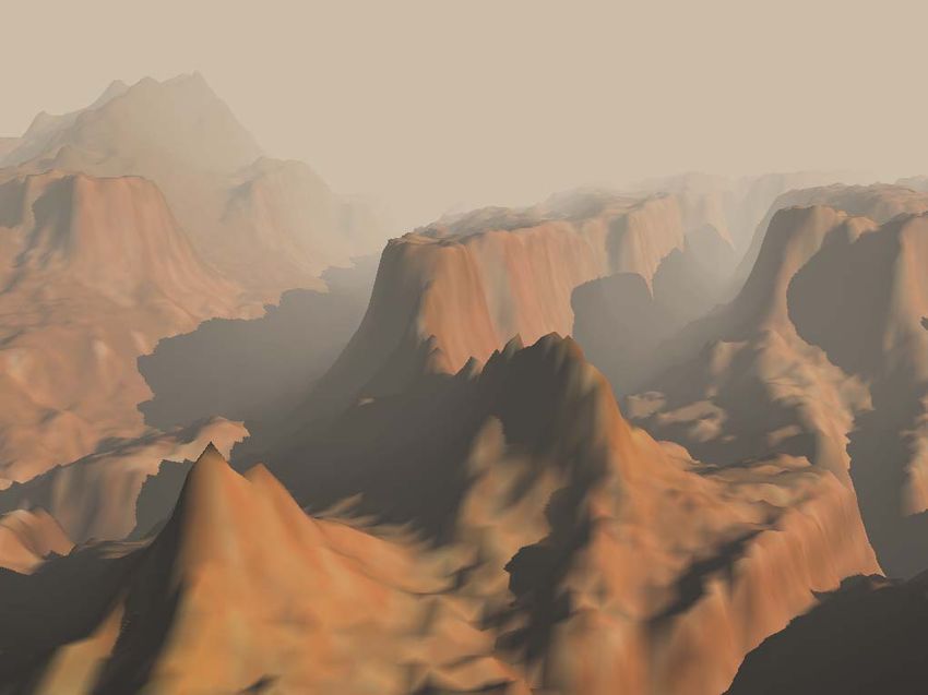
Cascaded Shadow Maps

                                    Document Change History

Version   Date   Responsible          Reason for Change
1.0              Rouslan Dimitrov     Initial release
1.1              Miguel Sainz         Figures and minor editorial fixes
Cascaded Shadow Maps

Shadow maps are a very popular technique to obtain realistic shadows in game engines.
When trying to use them for large spaces, shadow maps get harder to tune and will be more
prone to exhibit surface acne and aliasing. Cascaded Shadow maps (CSM) is a know
approach that helps to fix the aliasing problem by providing higher resolution of the depth
texture near the viewer and lower resolution far away. This is done by splitting the camera
                                                          view frustum and creating a
                                                          separate depth-map for each
                                                          partition in an attempt to make
                                                          the screen error constant.
                                                          CSM are usually used for
                                                          shadows cast by the sun over a
                                                          large       terrain.      Capturing
                                                          everything in a single shadow
                                                          map would require very high and
                                                          impractical resolution. Thus,
                                                          several shadow maps are used - a
                                                          shadow map that covers only
                                                          nearby objects so that each casts
                                                          a detailed shadow; another
                                                          shadow map that captures
                                                          everything in the distance with
                                                          coarse resolution and optionally
                                                          some more shadow maps in
                                                          between. This partitioning is
                                                          reasonable because objects that
                                                          are far away cast shadows that in
                                                          screen space occupy just a few
pixels and close-by objects might cast shadows that occupy a significant part of the screen.

Figure 1-1 shows a schematic of parallel split CSM, where the splits are planes parallel to the
near and far planes and each slice is a frustum itself. The sun is a directional light, so the
associated light frusta are boxes (shown in red and blue).
The algorithm proceeds as follows:
        •   For every light’s frustum, render the scene depth from the lights point of view.
        •   Render the scene from the camera’s point of view. Depending on the
            fragment’s z-value, pick an appropriate shadow map to the lookup into.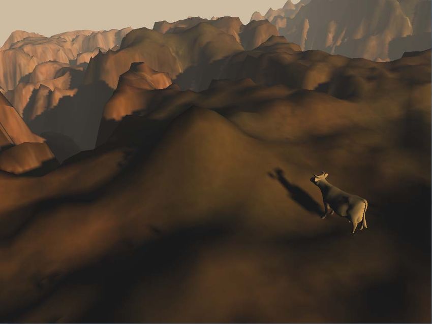
Cascaded Shadow Maps

 Figure 1-1. The right-most tree is captured in the near shadow-map and the other two are in the
 left. As seen from a viewer on the side, the left shadows are blocky, however, the camera would
                   perceive all 3 shadows with approximately the same aliasing.

Related Work
        There are several other popular approaches try to improve the screen-space aliasing
        error. The ones mentioned here traditionally work on the whole view frustum. Although
        these techniques can be applied to every frustum slice of CSM, this would not improve
        significantly the visual quality and comes with the expense of much greater algorithm
        complexity. In fact, CSM can be thought of a discretization of Perspective Shadow
        Maps.
        Perspective Shadow Maps (PSM) [2] – Figure 1-1 shows that part of the light’s frustum
        doesn’t contain potential occluders and is outside of the camera view frustum and this
        part of the shadow map is wasted. The idea behind PSM is to wrap the light frustum to
        exactly coincide with the view frustum. Roughly, this is achieved by applying standard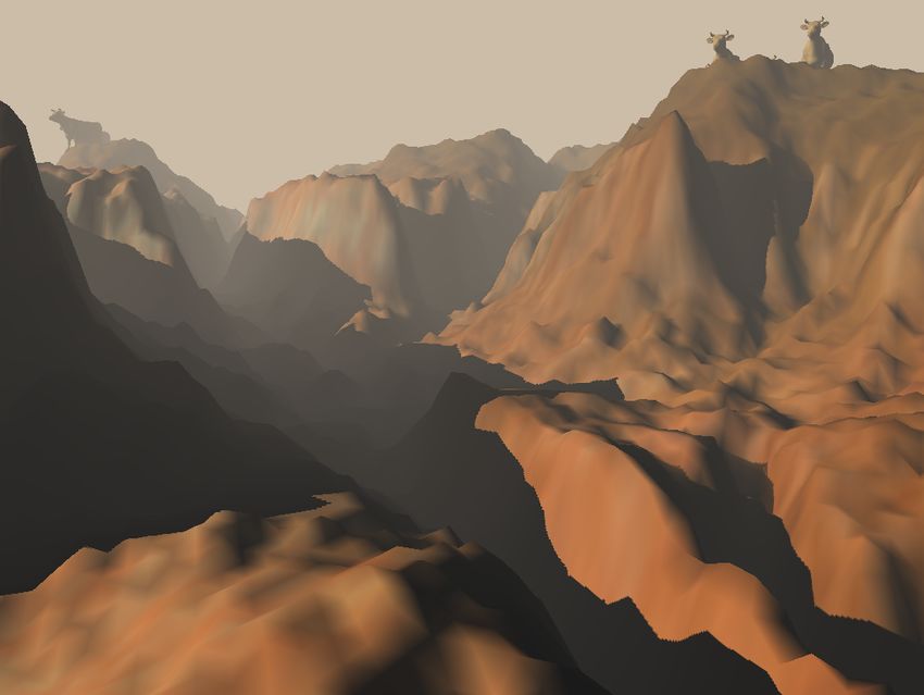
Cascaded Shadow Maps

       shadow mapping in post-perspective space of the current camera. A drawback of this
       method is that position and type of the light sources changes not intuitively and thus this
       method is not very common in computer games.
       Light Space Perspective Shadow Maps (LiPSM) [4] wrap the camera frustum in a way
       that doesn’t change the directions of light sources. A new light frustum is built that has a
       viewing ray perpendicular to the light’s direction (parallel to the shadow map). The
       frustum is sized appropriately to inclue the camera frustum and potential shadow
       casters. Compared to PSM, LiPSM doesn’t have as many special cases, but doesn’t use
       the shadow map texture fully.
       Trapezoidal Shadow Maps (TSM) [5] build a bounding trapezoid (instead of the frustum
       in LiPSM) of the camera frustum as seen from the light. The algorithm proceeds
       similarly to the other approaches.

Detailed Overview
       The following discussion is based on the OpenGL SDK demo on cascaded shadow
       maps and will explain the steps taken in detail.
       The shadow maps are best stored in texture arrays with each layer holding a separate
       shadow map. This allows for efficient addressing in the pixel shader and is reasonable
       since all layers are treated essentially in the same way.

Shadow-map generation
   By looking at figure 1-1, it can be noticed that everything outside the current light frustum
   (box) should not be rendered, provided that all shadow casters and the camera frustum slice
   are contained within it. In a way, the light’s frustum is a bounding box of the camera frustum
   slice, with near side extended enough to capture all possible occluders. If there were an
   occluder B (a bird, for example) above the trees, the boxes should be extended appropriately,
   or B wouldn’t cast a shadow.

                                 Figure 2-1. Camera frustum splits
   The first step of the algorithm is to compute the z-values of the splits of the view frustum in
   camera eye space. Assume a pixel of the shadow map has a side length ds. The shadow it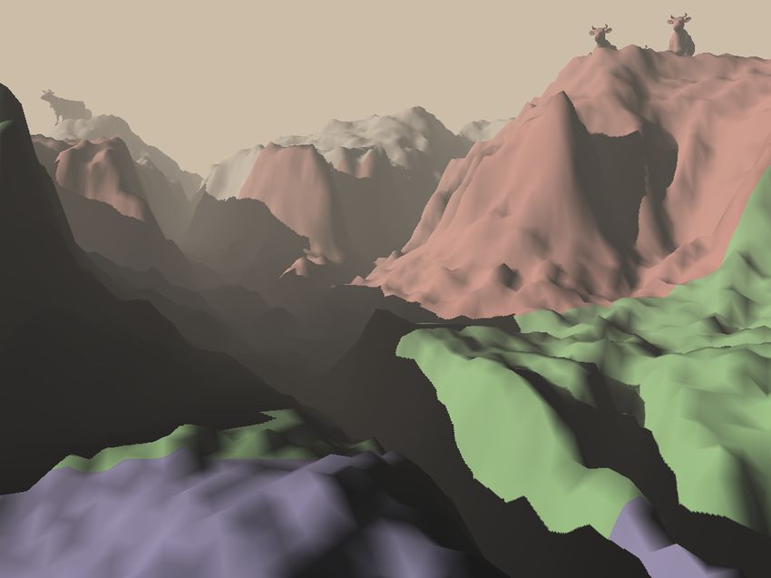
Cascaded Shadow Maps

casts occupies a fraction dp of the screen which depends on the normal and position of the
object being shadowed. Referring to diagram 2-1,
                                      dp    dz cos ϕ
                                         =n
                                      ds    zds cos θ
where n is the near distance of the view frustum.
In theory, to provide exactly the same error on the screen, dp/ds should be constant. In
addition, we can treat the cosine dependent factor also as a constant because we minimize
only the perspective errors and it is responsible for projection errors. Thus,
                             dz
                                 = ρ,                    ρ = ln( f / n)
                             zds
where the value of ρ is enforced by the constraint s ∈ [0;1] .
Solving the above equation for z and discretizing, (assuming the number of splits N is large),
the split points should be exponentially distributed, with:
                                        z i = n( f / n ) i / N
where N is the total number of splits. Please refer to [1] for a more detailed derivation.

                     Figure 2-2. Light frusta from light directly above the viewer

However, since typically N is between 1 and 4, the equation makes the split points visible
because the shadow resolution changes sharply. Figure 2-2 shows the reason for the
discrepancy: the area outside the view frustum, but inside the light frusta is wasted because it
is not visible; however as N → ∞ this area goes to 0.
Cascaded Shadow Maps
To counter this effect, a linear term in i is added and the difference is hardly visible anymore:
z i = λn( f / n) i / N + (1 − λ )(n + (i / N )( f − n) )
where λ controls the strength of the correction.
After the splits in z are known, the corner points of the current frustum slice are computed
from the field of view and aspect ratio of the screen. Refer to [3] for details.
Figure 2-3. Effect of the crop matrix and z-bounds change
Meanwhile, the modelview matrix M of the light is set to look into the light’s direction and a
generic orthogonal projection matrix P=I is set. Then, each corner point p of the camera’s
frustum slice is projected into ph = PMp in the light’s homogeneous space. The minimum
mi and maximum Mi values in each direction form a bounding box, aligned with the light
frustum (box), from which we determine a scaling and offset to make the generic light
frustum exactly coincide with it. This in effect makes sure that we get the best precision in z
and loose as little as possible in x and y and is achieved by building a crop matrix C. Finally,
the projection matrix P of the light is modified to P=CPz, with Pz an orthogonal matrix with
near and far planes at mz and Mz and
2
Sx =
Sx 0 0 Ox M x − mx
0 Sy 0 Oy 2
C = , Sy =
0 0 1 0 M y − my
O x = −0.5( M x + m x ) S x
0 0 0 1
O y = −0.5( M y + m y ) S y
Note that we can make the light’s frustum exactly coincide with the frustum slice, but this
changes the light’s direction and type as in perspective shadow mapsCascaded Shadow Maps
The scene is also frustum culled for each frustum slice i and everything is rendered into a
depth layer using (CPfM)i as modelview and projection matrices and the whole procedure is
repeated for every frustum partition.
Final scene rendering
In the previous step, the shadow maps 1…N were generated and are now used to determine
if an object is in shadow. For every pixel rendered, its z-value should be compared to the N
z-ranges computed before. For the following, assume it falls into the i-th range. Note that
the pixel shader receives this value in post-projection space, while it was originally computed
in eye space.
Then, the fragment’s position is transformed into world space, using the camera inverse
modelview matrix Mc-1 (which need not be a full inverse – the top 3x3 portion could be
transposed only if scaling is not used). Afterwards, it is multiplied by the matrices of the light
for slice i. The transformation is captured in the following composite matrix (CPfM)i Mc-1 .
Finally, the projected point is linearly scaled from [-1; 1] to [0; 1]. After all this transforms,
the fragment’s (x,y) position is actually a texture coordinate of the i-th depth map and the z-
coordinate tells the distance from the light to the particle. By doing the lookup we see the
distance from the light to the nearest occluder in the same direction. Comparing these two
values tells whether the fragment is in shadow.Cascaded Shadow Maps
Figure 2-4. A triangle casting a shadow in multiple depth maps
Code Overview
The accompanying OpenGL SDK sample contains the following source files:
• terrain.cpp – contains function definitions for loading and rendering the
environment. The only method needed for the shadow mapping algorithm is
Draw(), while Load() and GetDim() are called during initialization to load and
set the bounding box of the world properly.
• utility.cpp – contains many helper functions in order to make the main code
more readable. These include a shader loader; camera handling; menu, keyboard
and mouse handling, etc.
• shadowmapping.cpp – this file contains the main core code of the presented
algorithm and contains all code for creating and drawing the shadow maps and
the final image to the screen.
Roughly, terrain.cpp and utility.cpp provide the framework needed to run the sample
which in real games is provided by the game engine. In this analogy, display() is a part of
the rendering loop, which in this sample calls makeShadowMap() and renderScene().Cascaded Shadow Maps
Listing 3-1. An excerpt from makeShadowMap() (Slightly modified)
void makeShadowMap()
{
/* ... */
// set the light’s direction
gluLookAt(0, 0, 0,
light_dir[0], light_dir[1], light_dir[2],
1.0f, 0.0f, 0.0f);
/* ... */
// compute the z-distances for each split as seen in camera space
updateSplitDist(f, 1.0f, FAR_DIST);
// for all shadow maps:
for(int i=0; iDraw(minZ);
/* ... */
}
/* ... */
}
renderScene() sets the shader uniforms (see listing 3-2) and then renders the scene as it
would do without CSM. The important for CSM piece of code is in the pixel shader that
is applied during this pass.Cascaded Shadow Maps
Listing 3-2. shadow_single_fragment.glsl (Slightly modified)
uniform sampler2D tex; // terrain texture
uniform vec4 far_d; // far distances of
// every split
varying vec4 vPos; // fragment’s position in
// view space
uniform sampler2DArrayShadow stex; // depth textures
float shadowCoef()
{
int index = 3;
// find the appropriate depth map to look up in
// based on the depth of this fragment
if(gl_FragCoord.z < far_d.x)
index = 0;
else if(gl_FragCoord.z < far_d.y)
index = 1;
else if(gl_FragCoord.z < far_d.z)
index = 2;
// transform this fragment's position from view space to
// scaled light clip space such that the xy coordinates
// lie in [0;1]. Note that there is no need to divide by w
// for othogonal light sources
vec4 shadow_coord = gl_TextureMatrix[index]*vPos;
// set the current depth to compare with
shadow_coord.w = shadow_coord.z;
// tell glsl in which layer to do the look up
shadow_coord.z = float(index);
// let the hardware do the comparison for us
return shadow2DArray(stex, shadow_coord).x;
}
void main()
{
vec4 color_tex = texture2D(tex, gl_TexCoord[0].st);
float shadow_coef = shadowCoef();
float fog_coef = clamp(gl_Fog.scale*(gl_Fog.end + vPos.z),
0.0, 1.0);
gl_FragColor = mix(gl_Fog.color, (0.9 * shadow_coef *
gl_Color * color_tex + 0.1), fog_coef);
}
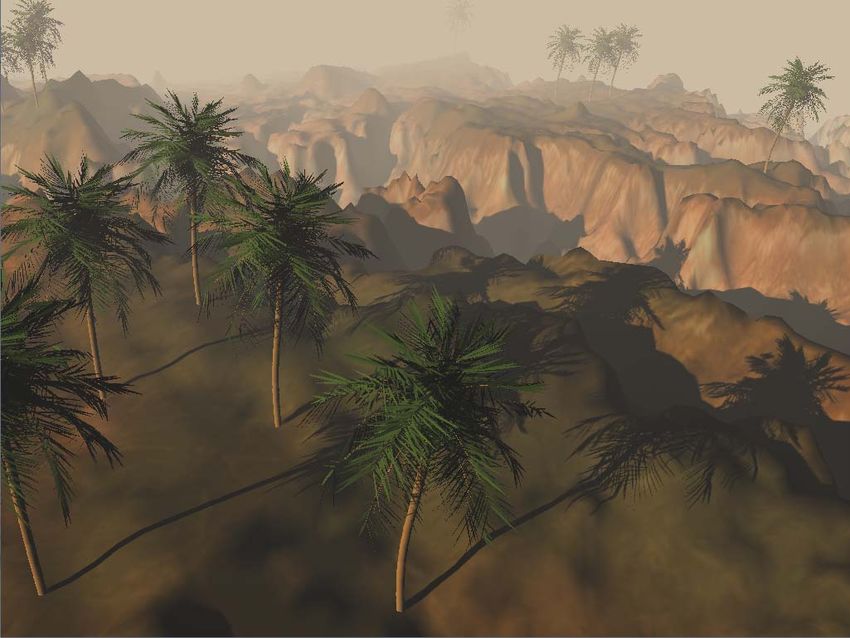
Results
This sections shows a few screenshots of large scale terrain rendering with 4-splits CSM,
where each shadow map is 1024x1024.Cascaded Shadow Maps
Figure 3-1. Large scale terrain rendering with 4-splits CSM
Figure 3-2. Texture look ups from different shadow maps are highlightedCascaded Shadow Maps
Figure 3-3. CSM with 1 split (note that CSM with 1 split provides better resolution than
standard shadow mapping because of the ‘zooming in’ by the crop matrix as explained
above)
Figure 3-4. CSM with 3 splits of the same sceneCascaded Shadow Maps
Figure 3-5. Another screenshot of the demo
Conclusion
Cascaded Shadow Maps are a promising approach for large scale environment shadows.
They do not suffer from many special cases and difficulties in treatment compared to other
warping methods and provide relatively uniform under-sampling error in screen space. Thus,
just by increasing the shadow map resolution, the jagged edges of shadows can be
significantly reduced for all objects in the scene, almost independent from their distance to
the viewer.Cascaded Shadow Maps
References
[1] Fan Zhang , Hanqiu Sun , Leilei Xu , Lee Kit Lun, Parallel-split shadow maps for large-scale
virtual environments, Proceedings of the 2006 ACM international conference, June 14-April 17,
2006, Hong Kong, China
[2] Marc Stamminger , George Drettakis, Perspective shadow maps, Proceedings of the 29th
annual conference on Computer graphics and interactive techniques, July 23-26, 2002, San
Antonio, Texas
[3] António Ramires Fernandes, View Frustum Culling Tutorial,
http://www.lighthouse3d.com/opengl/viewfrustum/
[4] Michael Wimmer, Daniel Scherzer, Werner Purgathofer. Light Space Perspective Shadow
Maps. Eurographics Symposium on Rendering 2004
[5] Tobias Martin, Tiow-Seng Tan. Anti-Aliasing and Continuity with Trapezoidal Shadow Maps.
Proceedings of Eurographics Symposium on Rendering, 21-23 June 2004, Norrköping,
Sweden
Terrain Reference
http://www.cc.gatech.edu/projects/large_models/gcanyon.html
Palm Tree Reference
http://telias.free.fr/zipsz/models_3ds/plants/palm1.zipNotice
ALL NVIDIA DESIGN SPECIFICATIONS, REFERENCE BOARDS, FILES, DRAWINGS, DIAGNOSTICS, LISTS, AND
OTHER DOCUMENTS (TOGETHER AND SEPARATELY, “MATERIALS”) ARE BEING PROVIDED “AS IS.” NVIDIA
MAKES NO WARRANTIES, EXPRESSED, IMPLIED, STATUTORY, OR OTHERWISE WITH RESPECT TO THE
MATERIALS, AND EXPRESSLY DISCLAIMS ALL IMPLIED WARRANTIES OF NONINFRINGEMENT,
MERCHANTABILITY, AND FITNESS FOR A PARTICULAR PURPOSE.
Information furnished is believed to be accurate and reliable. However, NVIDIA Corporation assumes no
responsibility for the consequences of use of such information or for any infringement of patents or other
rights of third parties that may result from its use. No license is granted by implication or otherwise under any
patent or patent rights of NVIDIA Corporation. Specifications mentioned in this publication are subject to
change without notice. This publication supersedes and replaces all information previously supplied. NVIDIA
Corporation products are not authorized for use as critical components in life support devices or systems
without express written approval of NVIDIA Corporation.
Trademarks
NVIDIA, the NVIDIA logo, GeForce, NVIDIA Quadro, and NVIDIA CUDA are trademarks or
registered trademarks of NVIDIA Corporation in the United States and other countries. Other
company and product names may be trademarks of the respective companies with which they
are associated.
Copyright
© 2007 NVIDIA Corporation. All rights reserved.
NVIDIA Corporation
2701 San Tomas Expressway
Santa Clara, CA 95050
www.nvidia.comYou can also read