Catching the Earworm: Understanding Streaming Music Popularity Using Machine Learning Models

E3S Web of Conferences 253, 03024 (2021) https://doi.org/10.1051/e3sconf/202125303024
EEM 2021

 Catching the Earworm: Understanding Streaming Music
 Popularity Using Machine Learning Models
 Andrea Gao1
 1Shanghai High School International Division Shanghai, China

 Abstract—The digitization of music has fundamentally changed the consumption patterns of music, such
 that the music popularity has been redefined in the streaming era. Still, production of hit music that capture
 the lion’s share of music consumption remains the central focus of business operations in music industry. This
 paper investigates the underlying mechanism that drives music popularity on a popular streaming platform.
 This research uses machine learning models to examine the predictability of music popularity in terms of its
 embedded information: audio features and artists. This paper further complements the predictive model by
 introducing interpretable model to identify what features significantly affect popularity. Results find that
 machine learning models are capable of making highly accurate predictions, suggesting opportunities in music
 production that could largely increase possibility of success within streaming era. The findings have important
 economic implications for music industry to produce and promote the music using controllable and
 predictable features tailored to the consumer’s preferences.

 store music in hard disks such as MP3 or iPods. The
 1 INTRODUCTION increasing prevalence of smart phones and the digitization
 of music prompted the establishment and wide usage of
 In the past century music production was mainly in the numerous music-listening apps such as Spotify, Google
 form of physical albums such as cassette tape and CDs. Play Music and Apple Music, among others, that gradually
 Singers and music producers record a list of song tracks to replaced CDs. Such switch of music consumptions, from
 sell as a whole set of physical album. As such, artists and purchasing physical albums to purchasing the single track,
 music industry heavily focus on maximizing album sales, not only changed the customer experience, but also
 which was one of the most critical measures of artists’ fundamentally changed the economics of the music
 popularity and business success [1]. Economically industry. For example, Apple pioneered the sales channel
 speaking, music can be considered as very similar type of through its iTunes store since 2001, a digital platform that
 goods like foods, movies, books. As an experience good, sells all tracks at $0.99. Consumers become much free to
 consumers don’t know the value and quality of the music choose which track to listen rather than purchasing an
 before purchasing. To resolve the uncertainty associated, album with the whole set of tracks, which is now
 consumers need to rely on other information – such as the independent of the price effect.
 music’s genre, fame of the artist, the album’s total sales Due to such a music industry evolution, Chris Anderson
 volume, and the music chart – as reference to make one’s (2004) proposed the long tail theory to characterize the
 choice. At the same time, consumers have to pay a high music consumption in digital era, in which a large portion
 search cost for the track they actually want since one album of tracks that were once unknown have gained certain level
 typically contains a curated list of tracks. To make the best of popularity altogether to form a long tail of the
 utilization of money, consumers tend to rely even more consumption distribution. This implies that the popularity
 heavily on the “other information” e.g., to leverage critic’s of the music and artists may spread within a larger range,
 rating and word-of-mouth popularity of the album, taking increasing sales of less known tracks from nearly zero to
 wisdom of the crowd when selecting music to purchase. few.
 Therefore, hit albums that have already accrued high sales More recently, the emergence of streaming platform
 figures will receive further more sales. In other words, the designs such as Netease Music, QQ Music, Pandora,
 sales of new music albums from popular artists may be Spotify, as well as the utilization of Artificial Intelligence
 amplified by the indirect information, but not the quality of into music recommendations have gradually exhibited a
 the music. This leads to a significant divide between artists spill-over effect [2] – music listened by other users with
 who may produce the music about the same level but end similar histories are recommended, thus increasing the
 up with vastly different levels of success. music popularity as it spreads from several users to a larger
 The 21th century has witnessed the technological group. This pushed a short list of tracks to become uniquely
 advancement in music industry that allowed consumers to popular. In 2018, Professor Serguei Netessine from

© The Authors, published by EDP Sciences. This is an open access article distributed under the terms of the Creative Commons Attribution
License 4.0 (http://creativecommons.org/licenses/by/4.0/).

E3S Web of Conferences 253, 03024 (2021) https://doi.org/10.1051/e3sconf/202125303024
EEM 2021

 Wharton University of Pennsylvania stated in his podcast controllable element in music production – composition.
 that, “We found that, if anything, you see more and more The results of this paper hope to give implications upon
 concentration of demand at the top”. Although the podcast how music in the current digital age, which popularity is
 focused on movie sales, experiences goods like theater and measured by streaming volume, can be composed to gain
 music sales occur in a similar fashion as shown in data the large volumes and thereby create economic value.
 distribution demonstrated in Section 3B. In the book “All Whether music in current ages have become more
 you need to know about the music industry” by Passman, predictable due to platform economics or the hope of
 he highlighted key differences between music business in producing an earworm is an important economic topic of
 the streaming era and record sales. [3] In the days of record interest that may cause large changes in the music
 sales, artists get paid the same money for each record sold, production industry.
 regardless of whether a buyer listened to it once or a In this paper, we aim to predict the popularity of tracks
 thousand times. But today, the more listens the music based on acoustic features, together with historic
 tracks have, the more money the artists make. Meanwhile, performance of artist. In particular, this paper includes
 records sales do not have strong spillover effects as fans of several state-of-the-art machine learning models that give
 different artists/genres will purchase what they like anyway. relatively implications of what features to what extent
 In fact, a hit album would bring a lot of people into record could make tracks become popular. Using a large-scale
 stores, and that increased the chances of selling other dataset, which incorporates more than 130,000 tracks from
 records. But in the streaming world, that’s no longer true. a world-leading music streaming platform Spotify, we
 The more listens one artist gets, the less money other artists adopted various advanced machine learning models to
 would make. In other words, the music consumption is intelligently classify which song tracks would have high
 undertaking a radical shift which may affect the definition popularity based on comprehensive audio features derived
 of popularity in the streaming era, however, it is yet from each track. This adds to the recent works that tried to
 severely underexplored. predict the music genres with audio features [9], in which
 Inspired by the evolution of music industry in the recent the machine learning models are used to categorize music
 decades and the recent debunk of long tail theory given a genres. In particular, we further introduced an explainable
 high concentration of popularity for a short list of tracks, AI tool as SHAP [10] to capture how these audio features
 this paper aims to investigate the popularity of music tracks have differential impact on the track popularity. As such,
 on streaming platform, largely different and not the presented results may provide strong implications to
 extensively explored about compared to that measured by understanding the popularity in the streaming music
 album sales, when it is impacted by the consumer choices platform and mechanism of essential audio features that
 and prevalent recommendation features. In particular, music industry may consider for production.
 rather than considering the level of advertisement, the The paper is presented as the following. The second
 inclusion in playlists of Billboard Hot 100 as Luis Aguiar section discusses previous works that analyzed the
 and Joel Waldfogel have noted, this paper focuses on economics of music industry and determinants of music
 leveraging music tracks’ inherent audio features – such as popularity. The third section introduces the Spotify dataset
 the key, loudness, tempo or measure of emotions to such as its features, categorical data assignments, and
 discover the underlying patterns that drive the popularity. general explorative data analysis demonstrations. The
 [4] Based on the concept of earworms [5] – catchy pieces fourth section explains several machine learning models
 of music that repeats through a person’s mind – come from used in this work in detail, – including Multiple Linear
 these tracks with uniquely high popularity, we hypothesize Regression, Logistic Regression, Decision Tree, Random
 that audio features may play an important role in Forest, and Boosting tree, and Neural Networks – the
 determining popularity. According to Seabrook (2016), the mechanism of the models, as well as the hyper-parameters
 music industry has transformed the business to produce used. Next, the fifth section presents the prediction results,
 tracks that have everyone hooked, through various means evaluates model performances, and interprets feature
 including marketing, technology and even the way the importance. Last, we discuss the implications of the
 human brains work.1 [6] For example, Jakubowski et al. research and conclude.
 discussed whether earworms have certain common-
 grounds or are composed according to certain formulas in
 a psychological lens, which gives inspirations of this paper 2 RELATED WORKS
 to study the similar subject matter from the lens of machine
 learning. [7] As streaming, or the number of listens, 2.1 Economics of Music
 becomes the main measure method of popularity, the cost
 of listening to music further decreases from individual In 2005, Marie Connolly and Alan B. Krueger, two
 songs to nearly none on some platforms as long as researchers from Princeton University, investigated the
 consumers have gained premier. Consumer’s freedom economics of the rock and roll industry. [11] They were of
 further increases and may listen to a song due to interest the first researchers who implemented economic
 and curiosity, and many todays believe that popularity is knowledge to study the subject matter of music. Connoly
 gained from information in social media [8]. Although and Krueger observed changes in the rock and roll concert
 many of other factors such as social media play a role in industry during 1990s, and explained how these changes
 determining music popularity, this paper provides an have contributed to factors like concentration of revenue
 additional perspective to the existing psychological or among performers and copyright protection. [1] As the
 platform studies, and provides suggestions for the most research was mostly descriptive and lies on the social
 Seabrook (2016) showed some anecdotal evidences that a company
 named Hit Song Science used a computer-based method of hit prediction
 that purported to analyze the acoustic properties and underlying
 mathematical patterns of the past hits.

 2

E3S Web of Conferences 253, 03024 (2021) https://doi.org/10.1051/e3sconf/202125303024
EEM 2021

 science research by concluding from massive survey 2.2 Determinants of Music Popularity
 results, the results, in the form of analysis, were valuable
 for studies but were neither numerical nor quantifiable. Some research in the more recent years have been
 In the more recent decade, an article named “Digital exploring similar topics – music popularity. Matthew J.
 music consumption on the Internet: Evidence from Salganik, Peter Sheridan Dodds, and Duncan J. Watts
 clickstream data” by Aguiar et al. [12] focused on the effect investigated the predictability of songs, stating that most
 of digital era and streaming on digital music sales. The successful are of high quality, most of the low-quality
 authors stated the “stimulating effect of music streaming on songs are unpopular, leaving the rest in between to be
 digital music sales” and that purchasing behaviors of unpredictable. [15] Moreover, Kelsey McKinney discussed
 customers have changed since 2000s due to the digital the history of track lengths’ changes in the recent decade,
 music platforms, largely statistical and economic. Music and concluded that song lengths between 3 to 5 minutes are
 industry revolution was also discussed in Hubert Léveillé more likely to become hit songs. [16]
 Gauvin that studied the compositional practices of popular Several papers have used machine learning models to
 music (number of words in title, main tempo, time before explain popularity by features. Askin et al. utilized
 the voice enters, time before the title is mentioned, and self- computer science tools to analyze the musical features of
 focus in lyrical content) and its changes with hundreds of nearly 27,000 tracks – including those in Hot 100 – and
 songs from U.S. top-10 singles in 1986~2015. [13] It shows concluded that tracks that are less similar to their peers are
 that popular music composition indeed evolves toward more likely to succeed, to some extent disproving the claim
 grabbing listeners’ attention, consistent with the “attention that popular music all sound alike and that earworms can
 economy” it proposes that the music industry has already be composed through certain formula. [17] This gives some
 transformed into. implication to the modeling process in this paper that linear
 In this paper, we build upon Aguiar and Martens’s models between features and popularity may not fit well,
 conclusion about the effects of digitization on platforms may require more complex models that capture the non-
 and investigate to what extent has this phenomenon caused linearity. Herremans et al. used basic musical features and
 people to have similar interests in music by looking several classification models to gain insight in how to
 specifically at most popular music. [12] This allows us to produce dance hit track, aiming to provide benefits towards
 testify some of the previous works, about whether music the music industry. While their work gives some insights
 interests have been converging due to music platforms’ to how popularity can be predicted and to what extent hit
 changes. Furthermore, instead of statistical analysis as in tracks can be produced, the models used in their work (ie.
 previous works, we utilize machine learning models Logistic Regression, C4.5 Tree, Support Vector Machine
 (logistic regression, random forest, neural networks, etc.) Classifiers) were relatively simple and basic, in which the
 to investigate trends in a large collection of diverse music features are not clearly explained. [14]
 tracks. Furthermore, Araujo et al., built upon the work by
 In the article “Platforms, Promotion, and Product Herremans, et al to predict whether a song would enter
 Discovery: Evidence from Spotify Playlists”, Aguiar and Spotify’s Top 50 Global ranking using classification
 Waldfogel analyzed streaming platform and promotion models. [14,19] It takes the platform’s previous Top 50
 techniques’ effects on music sales. [4] They specifically Global ranking as well as acoustic features into account and
 compared the difference in streaming volumes of tracks built upon several models, including Ada Boost and
 before and after they were added to global playlists as well Random Forests, probabilistic models with Bernoulli and
 as when tracks just entered and just left the top 50 popular Gaussian Naive Bayes, and multiple kernels for the
 list. They also aggregated the streaming volumes to Support Vector Machine classifier. Likewise, Interiano et
 observe effects of playlists on tracks’ popularity. The al. analyzed more than 500,000 songs released in UK
 effects were large and significant: adding the track to a between 1985 and 2015 to understand the dynamics of
 popular list called “Today’s Top Hits” may increase the success, by correlating acoustic features and the successes
 stream volumes of tracks by “almost 20 million that worth in terms of official chart top 100. [14] Their work also
 between $116,000 and $163,000”. Furthermore, inclusion showed the acoustic features has high predictability of the
 in “New Music Friday lists” generally raised possibility of success.
 success for tracks, regardless of the artist’s original
 popularity. Therefore, not only showing how platform 3 DATA
 economics such as streaming and playlists might have
 caused large effects on music popularity, this research
 further implies the huge economic value of successful 3.1 Spotify Dataset
 tracks, which increases the value of this paper’s purpose
 and results. In an economic lens, the predictability of music In the Spotify dataset, there are 130,663 tracks in total that
 popularity in terms of audio features, the most fundamental was collected in 2018 and 2019, respectively. For each
 and controllable elements of a song, is highly valuable for track, there are 14 numerical values in addition to the
 the industry. [14] track’s name and the artist. 13 of the numerical values are
 audio features, and the other is the label in this paper,
 popularity.

 3

E3S Web of Conferences 253, 03024 (2021) https://doi.org/10.1051/e3sconf/202125303024
EEM 2021

 3.1.1 Feature Explanation

 TABLE I. SPOTIFY DATASET FEATURE EXPLANATION

 Variable Description Mean Std.
 Dependent Var.
 popularity Overall estimated amount of streaming 24.209 19.713
 Audio Features

 duration_ms Duration of the track in milliseconds. 212633.1 123155.1

 Estimated overall key of the track using standard Pitch Class
 key 5.232 3.603
 notation. E.g. 0 = C, 1 = C♯/D♭, 2 = D, and so on.

 Modality (major or minor) of a track. Major is marked as 1, and
 Mode 0.608 0.488
 minor is marked as 0.
 Estimated overall time signature (notational convention about
 time_signature 3.879 0.514
 how many beats in each bar).
 Confidence measure of whether the track is acoustic. 1.0
 acousticness 0.343 0.346
 represents high confidence the track is acoustic.

 Suitability of a track for dancing based on a combination of
 musical elements including tempo, rhythm stability, beat
 danceability 0.581 0.190
 strength, and overall regularity. A value of 0.0 is least danceable
 and 1.0 is most danceable.

 Perceptual measure of intensity and activity. Typically,
 energetic tracks feel fast, loud, and noisy. For example, death
 metal has high energy, while a Bach prelude scores low on the
 energy 0.569 0.260
 scale. Perceptual features contributing to this attribute include
 dynamic range, perceived loudness, timbre, onset rate, and
 general entropy.

 Measure of whether a track contains no vocals. “Ooh” and “aah”
 sounds are treated as instrumental in this context. Rap or spoken
 word tracks are clearly “vocal”. The closer the instrumentalness
 instrumentalness 0.224 0.360
 value is to 1.0, the greater likelihood the track contains no vocal
 content. Values above 0.5 are intended to represent instrumental
 tracks, but confidence is higher as the value approaches 1.0.

 Measure in 0~1 of presence of an audience. Higher liveness
 liveness values represent an increased probability that the track was 0.195 0.168
 performed live.
 loudness Measure of average loudness of a track in decibels (dB). -9.974 6.544

 Measure of presence of spoken words in a track. The more
 speechiness exclusively speech-like the recording (e.g. talk show, audio 0.112 0.124
 book, poetry), the closer to 1.0 the attribute value.

 Measure of musical positiveness (ie. happy) in 0~1. Tracks with
 high valence sound more positive (e.g. happy, cheerful,
 valence 0.440 0.259
 euphoric), while low valence means tracks are more negative
 (e.g. sad, depressed, angry).

 tempo Estimated tempo of a track in beats per minute. 119.473 30.160
 Total Observations 130663
 Notes: In this table, “duration_ms”, “key”, “mode”, “time_signature”, “loudness”, and “tempo” are information directly extracted from the tracks. Also,
 “acousticness”, “danceability”, “energy”, “instrumentalness”, “liveness”, “speechiness”, and “valence” are values defined and calculated by Spotify
 according to certain internal algorithm.
 Source: Spotify Dataset2
 In other words, the popularity is based on both the volume
 3.1.2 Measurement of Popularity and regency of the streams.
 Generally speaking, tracks that are being played a lot
 According to Spotify’s website for developers, the
 recently will have a higher popularity than tracks that were
 popularity of a track is a value between 0 and 100, with 100
 played a lot in the past. Duplicate tracks (e.g. the same track
 being the most popular. The popularity is calculated by
 from a single and an album) are rated independently. Artist
 Spotify’s internal algorithm and is based on the total
 number of plays of the track and how recent those plays are.

 4

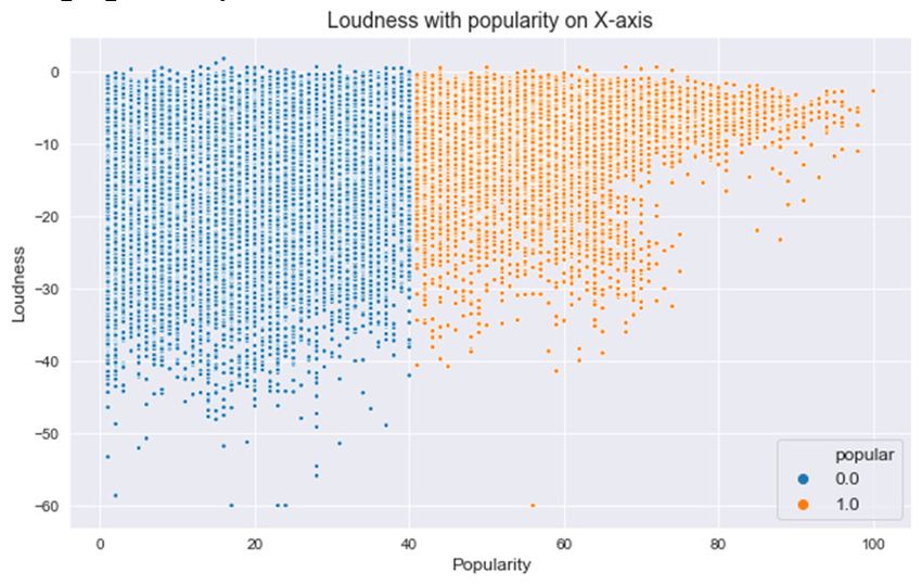
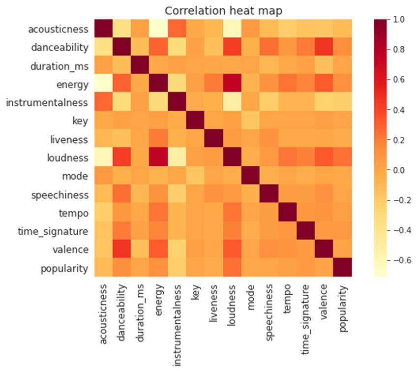
E3S Web of Conferences 253, 03024 (2021) https://doi.org/10.1051/e3sconf/202125303024
EEM 2021

 and album popularity are derived mathematically from increasing number of songs with increasing popularity,
 track popularity. called a chasm.
 Given that track popularity can be directly measured at As we acknowledge that there is a large range of tracks
 the streaming platform as the function of number of listens, that have extremely low popularity, even zero according to
 in comparison to the past times, when music was sold as Spotify’s calculation algorithm, it is not sensible to study
 physical albums. For example, the presence of pirated this as a regression problem and predict specific popularity
 albums as well as the unknown number of listens makes the of songs. As seen in this Figure, the chasms serve as
 official number of album sales inaccurate for the real thresholds, above which the number of tracks with higher
 popularity. This is one significant advantage of digitization popularity continuously decreases. Most songs that cannot
 which provides much more accurate measurements of pass such a threshold and enter the decreasing trend can
 popularity than the old days. rarely be successful. Therefore, rather than predicting
 specific popularities of songs, we can classify the songs
 into popular and unpopular. An interesting fact is that the
 3.2 Explorative Data Analysis and Data
 lowest point of the chasm at around popularity of 25 marks
 Standardization
 exactly 50% of all songs. In other words, exactly 50% of
 In explorative data analysis, we used histograms of features, songs have either passed or have popularity below 25.
 a correlation heat map of all features included, as well as Therefore, as we hope to focus solely on those songs that
 bar graphs and scatter plots with simple regression lines of have succeeded and passed through such threshold that
 several features with popularity. become successful, the labels for classification models in
 this investigation are set such that the tracks with top 25%
 in popularity are classified as popular, and the remaining
 75% are unpopular. The reason to set 25% as the
 classification boundary is to ensure that tracks above this
 level are really those that have succeeded, having passed
 the chasm with a large extent. The tracks with popularity
 of zero are removed before classification since they do not
 receive any interaction with the users. The benchmark was
 calculated to be at 41, as 25% of the non-zero-popularity
 tracks have popularity larger or equal to 41. The popular
 tracks are marked as 1 while the unpopular are marked as
 0.

 Figure 1. Visualizer Popularity Distribution Before Scaling

 This appears to support the long tail theory on first
 glance, as a large majority of the tracks have extremely low
 popularities at about zero and a nearly unseen portion of
 tracks have high popularity between 80 and 100. To make
 the results more valuable, we include only songs that are at
 least listened to an accountable number of times, we
 excluded the songs with popularity of 0.

 Figure 3. Correlation Heat Map of Spotify Features

 The figure above shows a heat map that demonstrates
 the correlation between features pairwise. The larger direct
 correlation, the darker colors, or larger heat, of the small
 square. From this figure, we can grasp a general trend of
 Figure 2. Popularity Distribution, After Removal of Zero
 Popularity Tracks which features may be correlated. For example, loudness,
 or the average decibel of a piece, has a close correlation
 After excluding tracks with popularity of 0, the tracks’ with energy as denoted by the dark red square, while
 popularity distribution visually differs from what is stated energy and acousticness don’t have as strong a correlation
 by long tail theory, or a strictly inverse relationship as shown by the light-yellow colored squares that is close
 between popularity and the number of songs with that to white. Note that for loudness, if a piece has occasional
 popularity. In this graph, there are instances where there are large volume or largely fluctuating volume as seen often in
 symphonic music, which has large dynamics in volume,

 2
 More information of Spotify Dataset can be found on this website:
 https://developer.spotify.com/documentation/web-
 api/reference/tracks/get-audio-features/

 5

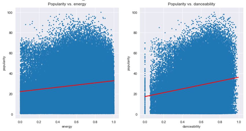
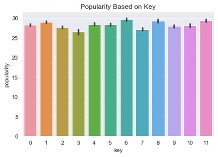
E3S Web of Conferences 253, 03024 (2021) https://doi.org/10.1051/e3sconf/202125303024
EEM 2021

 then its loudness would be relatively low as Spotify time signatures might naturally sound not as attractive,
 calculates it as an averaged value; if a song is of consistent implying that tracks with time signature of 4 may generally
 high volume, then its loudness would be relatively higher. have higher popularity and possibility to succeed.
 Focusing on popularity, we can see that the features’
 correlations with popularity are generally moderate, while
 instrumentalness has the weakest and loudness has the
 strongest correlation. This serves as a reference when
 evaluating models as we have in mind what features may
 affect popularity more.

 Figure 6. Bar Plot of Average Popularity Based on Key

 In the graph above, we see the bar graph of average
 popularity for tracks with each key. Key is one of the most
 Figure 4. Scatter Plot of Popularity and Loudness
 basic features within the composition of a piece of music.
 As one of the most fundamental features that can be
 Using the classification method of popular and changed for a track easily by modulating from one key to
 unpopular tracks in the previous sub-section, the tracks are another, one may expect average popularity of tracks from
 colored accordingly with orange and blue representing each key to be on a relatively similar level if they are really
 popular and unpopular tracks respectively. According to unaffecting popularity. However, in this plot, we observe
 this graph with popularity on the x-axis and loudness on the some relatively considerable differences in the average
 y-axis, there is a clear trend that the orange popular data popularities. For example, average popularities of key 6, 8,
 points generally have higher loudness, suggesting possible and 11 are higher than those of keys 3 and 7. This might
 relationships between the two factors that popular tracks imply that keys do have certain effects on popularity, which
 generally are louder overall. According to loudness’s would be further explored later in the Results section.
 definition and its implications, this shows that tracks with
 large dynamics in loudness might not be as popular as those
 with more stable and large volume.

 Figure 7. Bar Plot of Average Popularity Based on Key

 In the plots of popularity against energy and
 danceability respectively, both plots suggest that a
 moderately higher energy and danceability have the highest
 popularity values, while this trend is clearer between
 Figure 5. Bar Plot of Average Popularity Based on Time popularity and danceability as low danceability barely has
 Signature any popular tracks, which is not seen in the plot for
 popularity and energy. When specifically observing values
 Above is the graph of the average popularity for tracks of energy and danceability of those songs with especially
 with certain time signature, or the number of beats at each high popularity, larger values of these two features appear
 bar in a certain piece of music. This bar graph shows that to be the majority.
 the average popularity of tracks with time signature of 4 is Other than explorative data analysis, we also wanted to
 generally higher than tracks of other time signatures. 4 is a use artists’ names as a categorical feature. It is normal to
 very ordinary and commonly used signature used in all recognize that some tracks are famous due to the singer’s
 kinds of music. On the other hand, only rarely are 5 beats popularity, while the internal features of the tracks are not
 per bar used in popular music because it generally produces as important. Therefore, we divided all singers into 4
 an awkward rhythm for listeners. From Figure 5 we can see groups, according to the number of songs they have in the
 that the most common and popular 4 beat per bar might be dataset. Artists of the least 25% number of tracks is labeled
 more preferred by music consumers, while those unusual

 6

E3S Web of Conferences 253, 03024 (2021) https://doi.org/10.1051/e3sconf/202125303024
EEM 2021

 “first”, 25% to 50% labeled “second”, 50% to 75% labeled 4 MACHINE LEARNING MODELS
 “third”, and the rest labeled “fourth”. Thereby, we have a
 quartile variable that measures whether certain artists are After preparing the dataset with comparable features and
 experienced. certain noticeable correlations, the next step is to train high
 We noticed that the number of tracks of artists cannot quality models and continuously improving upon them
 directly tell the artists’ popularity while we expect an through hyper-parameter tuning and Principle Component
 artist’s popularity to large affect the songs this artist Analysis (PCA) to create the model that produces the best
 produces in the future. Therefore, we brought in a similar results.
 dataset as the Spotify dataset we are mainly using, but from In this paper, multi-variate linear regression, logistic
 an earlier time – the main dataset is from April 2019, while regression, and decision tree are the baseline models on
 this similar dataset is collected in November 2018. Note which we hope to utilize different methodologies to
 that the Spotify internal algorithm take only streaming in a improve upon and distinguish the most influential features
 short time frame into account, these two datasets have that make music popularity predictable.
 tracks with largely different popularity. The number of
 popular tracks in this similar November 2018 dataset, 4.1 List of models used in this work
 calculated with similar methods as detailed in previous
 sections, is counted for each artist, and all artists with at
 least one popular track are classified into quartiles with an 4.1.1 Multi-variate linear Regression
 additional category for those artists without any popular
 tracks. This additional feature marks tracks in the main Multi-variate linear regression is one of our baseline
 dataset with artists without any popular songs in the models in this paper. It is a simple regression machine
 November 2018 dataset as “first”, the tracks with artists of learning model that predicts numerical values by giving
 bottom 25% in number of popular tracks as “second”, etc. each feature a weight that denotes how it affects the
 until “fifth” for tracks with the artists with top 25% number dependent variable, which is popularity in this case.
 of popular tracks in the November 2018 dataset. Least-squares regression sums the squares of the
 Other than the plots shown above, the explorative data residuals and finds the coefficients minimize the sum. It
 analysis results as well as visualizations of all features are prevents the errors with opposite signs from cancelling out,
 given in Appendix A. thus creating fairer regression results. [2] For this linear
 Finally, for more comparable results and to ensure one regression, the total sum of squares of the vertical distance
 feature doesn’t affect the dependent variable too much, we between the line and each data point is called the cost
 scaled all features including popularity to a scale of 0~1. function, or least-square error (LSE) function, which is
 hoped to be minimized. The equation is � � � ∙ , in
 which � is a vector of all predicted values; � is the
 3.3 Training and Testing Data transpose of the vector of coefficients in the multivariate
 regression equation, which is a row vector; and is a
 After explored some information implied in the data such
 matrix of all data, including values of all features for each
 as correlation between different features and added
 data point. [20] The cost function is
 potentially helpful categorical features, it is important to
 � � � ��� � ∑� �
 ���� ∙ 
 ���
 � ��� �� (1)
 prepare data to be used in models.
 First, as our classification method separates tracks into To find the vector that minimizes this cost function
 popular and unpopular ones, the former includes 25% � �, we used the normal equation method to do this work.
 while the later includes 75% of all tracks. This causes the [20]
 two classes to be unevenly distributed. To solve this Since the value outputs are continuous, we used a
 problem, we used undersampling to balance the two classes consistent classification method as detailed in section 3.
 by randomly selecting the same number of samples from Popularity of larger than or equal to 0.41 (scaled) is popular.
 negative class as that in positive class. After undersampling,
 there are 32983 samples in each of the positive and 4.1.2 Logistic Regression
 negative classes.
 Furthermore, each model is trained on a training set and Logistic regression is another baseline model used in this
 tested on a testing set. From the 65966 samples in total, 80% paper. It is a simple classification model that predicts the
 are randomly chosen as the training set and the remaining possibility of some instance falling into binary classes of 0
 20% of samples are the testing set. This allows the test the or 1, defined in this paper as unpopular or popular tracks.
 generalizability of models by observing whether the model If the possibility calculated is larger than 50%, then the
 predicts the label, popularity in this case, successfully as instance is classified as 1; if not, it is classified as 0.
 measured by the evaluation metrics. As generalizability is To fit the continuous output values (as in linear
 one of the most crucial factors considered in the model, the regression) within the range of 0~1, the sigmoid function
 �
 split of data into training and testing subsets evaluates ℎ� � � � �� � � � ���� ��
 is used. This transfer
 ���
 whether models predict successfully, thereby implying function bounds the output to a “S” shape curve within 0~1
 whether models can accurately and realistically show the as shown in the following figure. We interpret the output
 determinants of tracks being popular. as a probability predicted from a range of input values
 represented by � .

 7

E3S Web of Conferences 253, 03024 (2021) https://doi.org/10.1051/e3sconf/202125303024
EEM 2021

 prediction that allows humans to interpret how the results
 are predicted, which is one of its advantages.
 We directly used Decision tree method in ski-learn,
 which implements the Classification and Regression Trees
 (CART) algorithm, the latest version until now.
 The cost function of decision tree is utilized at every
 level within the model. The set at each node is split into
 ����� ������
 two subsets using � , � � � � ���� � � ����� ,
 where left/right denote each of the two subsets, ����/�����
 measures the impurity of the corresponding subset, is
 the number of total samples, and ����/����� is the number
 of samples within the corresponding subset. Once the set is
 split into two after minimizing this cost function, the
 algorithm continues until the maximum depth is reached,
 which is a hyper-parameter, or when it cannot continue
 splitting to reduce impurities. [20]
 Figure 8. Sigmoid Function3
 Note that the decision tree algorithm is a greedy
 algorithm, meaning that it splits the current set to minimize
 Similar as linear regression, logistic regression also has the current level’s impurities but does not consider the
 a cost function that is minimized to find the coefficients . impurities several levels down. This may imply that
 In logistic regression, the method is called Maximum Decision tree is not being the optimal model.
 Likelihood Estimation. [20] The log loss function is
 �
 1
 � � � � � ��� � � ��� � 4.1.4 Random Forest
 
 ���
 ���
 ��1 � �log �1 � � � ��� �� (2) Random forest is a model that uses bagging on multiple
 ��� CART Decision trees. In other words, random forest builds
 in which is the real label value. The loss function
 multiple Decision tree models in parallel and uses
 serves its role by increasing in value if the predicted value
 “majority votes” to get a more generalizable, more accurate,
 ℎ� � ��� � is largely different from ��� . By repeatedly and more stable model.
 calculating the partial derivative of the loss function, � is First, the bootstrap method randomly selects training
 updated after each iteration, denoting the current subsets with replacement from the entire dataset. Those not
 integration. selected, taking about 1/3 of total samples, are “out of bag”
 � � (OOB) samples that are called out by the OOB method in
 � � �
 � ski-learn. Since they are never used in training, they readily
 � �
 � ∑���� � � � � � � ��� ��� ���
 (3) test the model, and the method of reserving a subset for
 �
 � testing is no longer needed.
 � � ��� � ∑� � � ��� � � ��� � � ��� (4) On each sample, random forest builds a decision tree
 � ��� �
 in which represents the learning rate hyper-parameter. If using only a subset of all features. This increases the
 the partial derivative is positive, the loss function is randomness within the model, which leads to more robust
 increasing, then next � is reduced; if negative, then overall predictions. The individual models work in a
 increasing the next set of parameters would possibly result similar recursive mechanism as detailed for Decision tree.
 in lower loss. This process is repeated until convergence. At last, after results are produced for each sample, the
 In scikit-learn, we utilize the built-in Logistic Regression “majority votes” method is used to vote out the final
 model to employ such a process. prediction by aggregating all predictions from the decision
 L2 Regularization is used to eliminate outlier weights trees. Each decision tree gives the probability that the
 which may occur during the training process. An additional instance is a popular track, and the “majority votes” method
 �
 ∑� � is added to the loss function called the averages this probability to give final classification results.
 term
 �� ��� � [20]
 penalty term. This term increases the cost when there are As a whole, random forest is more preferred compared
 outlier weights, thereby forcing the outlier weights lower to decision tree due to its larger diversity and randomness
 to an average level. [20] This increases generalizability of that prevents the problem of over-fitting and increases
 the model. model accuracy by voting, which disregards instances of
 bad predictions. Very uncorrelated trees will grow from
 4.1.3 Decision Tree each sample and adds to the diversity of the forest.
 However, its interpretability is lower as affected by its
 Decision tree is a supervised machine learning model for complexity.
 classification or regression usage. In our paper, we use the
 Decision tree classifier model for consistency. Decision
 tree, as its name implies, allows the prediction of certain
 values by following the decisions throughout the tree from
 the root to the leaf nodes. This stepwise and white box
 3
 Picture come from
 hvidberrrg.github.io/deep_learning/activation_functions
 /sigmoid_function_and_derivative.htm

 8

E3S Web of Conferences 253, 03024 (2021) https://doi.org/10.1051/e3sconf/202125303024
EEM 2021

 4.1.5 Boosting Tree models that do not solely fit linear relationships may be a
 better for this investigation.
 Boosting Tree Explanation: Boosting tree is a Neural network includes layers of “artificial neurons”
 classification model similar with random forest such that that originated from the structure of biological neurons and
 they both utilize Decision trees. However, boosting tree were extended to methods of machine learning. In a Multi-
 doesn’t run trees in parallel and there is no voting process. layer Perceptron (MLP) model, one single neuron from one
 Boosting tree is a sequential tree model that each learner in layer accepts input from other neurons from the previous
 the sequence improves upon the previous training results layer, processes it, and passes to another on the next layer.
 by increasing the weight of errors and thereby trying to This creates a feedforward artificial neural network.4
 learn these errors within each iteration. In each single neuron, input values are weighted, and
 Each model is trained sequentially first, starting with a the sum passes through an activation function. The hidden
 model having equal weights and then adding weights to layer’s neurons obtain the results from the previous layer,
 errors from the previous model. After each classifier is and passes on until meeting the end of all layers. Two other
 trained, each is assigned a weight such that more accurate layers – input layer and output layer – don’t do any
 classifiers are assigned larger weights. The weight is calculation work but simply pass the data in and out of the
 � ���
 calculated by � � ln � ��, in which � is the weights system. By MLP, neural networks are able to predict
 � ��
 of the �� classifier and � is the weighed sum error for linearly inseparable relationships.
 misclassified points, based on the classifier’s error rate. As In our model, we implemented the ReLU (Rectified
 a result, the final classifier model is just a linear Linear Unit) activation function in inner layers, which is
 combination of all the individual classifiers’ output times currently the most used activation function throughout the
 weight of each classifier. world right now. ReLU creates a threshold such that all
 � � � ∑���� � ℎ� � � (5) input values below it will output 0, which allows the
 in which ℎ� � � is the output of the �� classifier (XGBoost network to converge must faster and creates a more
 practically and computationally efficient model. The final
 Documentation).
 layer utilizes a Softmax function that assigns probabilities
 Boosting Tree and PCA: With the boosting tree model, � ��
 we used PCA, or Principle Component Analysis, to reduce to each class by �� � ��� � � � � � �� in which �
 ∑� �
 features of the model and project it to a lower dimensional
 represent that value of the �� instance in the previous layer.
 space. Sometimes, overfitting is caused by high dimensions,
 In addition, in the input and hidden layers, a bias node is
 or in other words large number of features, and the fact that
 added to shift the activation function to the right or left to
 they are intercorrelated, which makes the weight of certain
 fit the data. As a whole, the output is calculated with the
 features diverge from their real contribution to the model.
 formula ��� � � � � � ∑� � � � � ∑� � �� � �� �, such
 PCA prevents these interrelationships between features.
 PCA works by first identifying a hyperplane. The data are that ∑� � �� is the summation at one node in �� for its
 normalized, and PCA calculates the covariance matrix of inputs times weight, �� is the weight connecting layer 
 the features involved. Eigenvalues and eigenvectors of the and , � is the activation function for this �� layer, is
 covariance matrix is then calculated, and the original data the bias term in each layer, � is the activation function for
 is multiplied with the eigen vectors which suggests the output layer, or the �� layer. By such a computation fed-
 directions of the new axes. Then, the calculation results are forward layer by layer, the final output is calculated.
 plotted, which demonstrates how closely related the data The cost function of neural networks uses the sum of
 are. square errors, which is calculated at the end of the model.
 As a model using PCA is relatively unexplainable since Similar as previous models, we hope to find the optimizing
 the principle components don’t have real world meaning as set of weights and bias in each layer that minimize
 the original data do, the performance of the classification ����� � ∑��� � � � � � .
 �
 model using PCA components can be visualized by using To minimize the error, we use gradient descent to
 TCSEVisualizer. The visualizer and PCA decrease reduce error iteratively. New weights are obtained through
 dimensions of the data and show how well the test samples moving the original weights along the multi-dimensional
 are predicted by using colors to denote popular or ��
 space with the formula �� ��� � �� ��� � � . A
 unpopular tracks, thereby showing how well the two ����
 groups are discriminated. The results give suggestions for negative gradient increases weights and moves towards
 whether predictability exists within music’s popularity, a possible lower loss; a positive gradient decreases weights
 largely intangible measurement. and also move towards the global minimum.
 To find the optimizing set of weights, neural system
 uses backpropagation algorithm. This algorithm starts with
 4.1.6 Neural networks
 the output layer , and then to , , and so on, which back-
 Neural networks are a model that is theoretically best used propagates the error to previous layers and calculates the
 for highly nonlinear systems, but also easily overfits. As error at each output node including the hidden layers. The
 mentioned in Section 2, listeners nowadays tend to prefer following calculates the partial derivative of error function
 music of higher diversity, so we hypothesize that there is with respect to parameters between layers � 1 and .
 ��
 hardly a linear trend between each feature and popularity � ��� � (6)
 �����,�
 since very popular music may have largely diverse audio
 features. In this case, neural network and some previous

 9

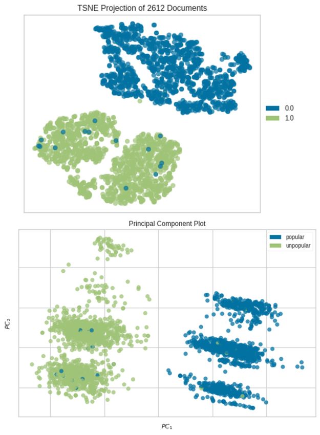
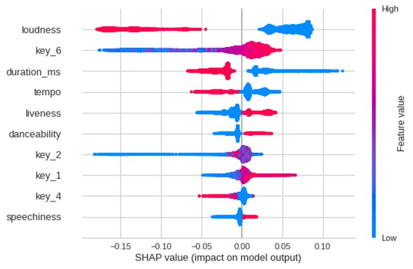
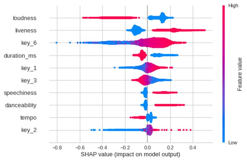
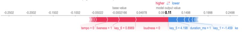
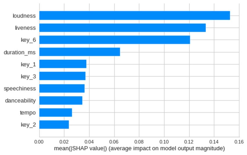
E3S Web of Conferences 253, 03024 (2021) https://doi.org/10.1051/e3sconf/202125303024
EEM 2021

 In the equation, � represents the back-propagated error evaluation metrics are derived from the confusion matrix,
 term on node , and ��� represents the output on node � while F1 is a combined score of precision and recall. Given
 1, which is the previous node. Thereby, parameters are that our labels are highly imbalanced, the commonly used
 updated until the final output’s loss converges. [21] accuracy measure may yield misleading interpretations.
 Therefore, we decide not to include accuracy as the
 evaluate metrics of all models.
 4.2 Hyper-parameters Tuning
 TABLE II. CONFUSION MATRIX
 For tuning hyper-parameters, we used GridSearchCV from
 ski-learn to evaluate different combinations of the values Predicted Positive Predicted Negative
 for these three hyper-parameters through cross validation Actual Positive True positive (TP) False negative
 and derive the best one that yields best evaluation results. (FN)
 GridSearchCV is a function that splits the training set into Actual Negative False positive (FP) True negative (TN)
 5, and each set of hyper-parameters is used to train the set
 on four of the subsets and tested on the other. The average
 4.3.1 Accuracy
 score of five fitting results for each combination of hyper-
 parameters are compared, and the best combination is Accuracy �
 �����
 (7)
 chosen. The cross-validation method prevents over-fitting �����
 and bias due to smaller datasets since the model is trained Accuracy denotes the proportion of number of correct
 on different subsets and averaged. predictions out of total predictions. This is one of the most
 After using GridSearchCV and fitting the training sets, straightforward measurements of a model’s performance
 we call “best_params_” that gives the set of hyper- by assessing the general correctness of the model’s
 parameters that created best-performing models. [20] predictive results. In fact, accuracy doesn’t vary much
 In Logistic Regression, we tuned the hyper-parameter across all models. Furthermore, we only want to focus on
 “C” which denotes the “inverse of regularization strength”, the tracks that are popular and according to what features
 or a measure of the inverse of constant within the cost the models assign the tracks as popular is what interests us.
 function. The larger “C” the stronger regularization. This Therefore, other metrics are relied on more to effectively
 parameter helps eliminate outlier weights and thereby evaluate the models’ prediction results.
 increases generalizability of the model.
 Decision Tree has a few hyper-parameters, including 4.3.2 Accuracy
 “max_depth”, which is the maximum iterations that can
 ��
 occur or the maximum layers the decision tree has; Precision � (8)
 �����
 “min_samples_split”, or the minimum samples required to Precision measures the proportion of real positive instances
 split an internal node; as well as “min_samples_split”, the that are successfully predicted out of all predictions of
 minimum number of samples required at one node after positive instances. In this paper, precision denotes the
 each split. An overly large maximum depth may make the proportion of actually popular tracks within all tracks that
 model overfit the data and reduce its generalizability, while are predicted as popular. Since what we want to focus on
 overly low minimum splits may lead to meaningless levels. are the features that lead to high popularity of tracks, this
 [20] precision score is very important as a higher precision score
 In Random Forest, first, “max_depth” and shows that the model has found the characteristics of
 “min_samples_leaf” are also used; “n_estimators” is the popular tracks that allows it to correctly predict what tracks
 number of trees in the forest. In general, the larger are popular.
 “n_estinators” means that there are more trees within the ��
 Recall � (9)
 forest, implying that the majority voting strategy would �����
 help eliminate more errors occurring in some of the Recall measures the proportion of predicted positive
 individual tree models. [20] instances out of all positive instances, meaning the
 In Boosting Tree, considering the complexity of proportion of popular tracks that are successfully predicted
 boosting tree which takes a long running time, “max_depth” as popular out of all popular tracks. A higher recall score
 and “n_estimators” are two main hyper-parameters that are in this paper means that the model is able to fetch a large
 tuned carefully. Learning rate is set to 0.005 as a typical number of tracks as popular out of the entire pool, meaning
 value. “subsample” is the proportion-wise sample size of that the traits of tracks that the model finds that determine
 the entire sample used during each iteration, which is tracks to be popular are can be applied to many of those
 typically set to 0.5. [20] popular tracks. Therefore, the model can recognize a wider
 Different from other models, neural networks require range of popular tracks, possibly of different types. This
 manually creating the model parameters including learning makes the model more comprehensive and therefore
 rate, the number of nodes in each layer, the number of valuable.
 layers, as well as the activation function.
 4.3.3 F1 score
 4.3 Evaluation metrics ����������������
 F1 score � 2 � ���������������� (10)
 The evaluation metrics used in this paper include the While there is usually a tradeoff between the precision and
 following: precision, recall, and F1 score. The former three recall scores, the F1 score provides a combined score of the
 4
 Basheer, Imad & Hajmeer, M.N. Artificial Neural Networks:
 Fundamentals, Computing, Design, and Application. Journal of
 microbiological methods. 43. 3-31. 10.1016/S0167-7012(00)00201-3.
 [22]

 10

E3S Web of Conferences 253, 03024 (2021) https://doi.org/10.1051/e3sconf/202125303024
EEM 2021

 harmonic mean for the two, and gives a suggestion for what explain in what direction and magnitude each feature
 combination of precision and recall may create a best affects the prediction, thereby transforming numerical
 model. This F1 score allows us to choose from a range of values into real-world meanings, specifically explaining
 models that have different levels of precision and recall that what features in what direction and how strongly affect
 none of the models have absolute advantage over others in popularity of tracks. All of this information is summarized
 both of the evaluation scores. [20] This is also especially in the SHAP Summary Plot. In the plots, red and blue
 useful when both recall and precision are important in our means high and low feature values respectively. The
 model and models with different combinations of the two horizontal axis means negative or positive SHAP values
 score are difficult to compare. from left to right, denoting negative or positive influence
 of certain feature values on the label value, or popularity.
 We also created force plots built within SHAP in python.
 4.4 Model Interpretation Tools – SHAP
 The force plots show how strongly each feature affects a
 certain predicted value. This implies each feature’s
 4.4.1 SHAP value importance in predicting the label that models real world
 instances, thereby showing whether there are and what
 Once we have trained the best performing models, features are deterministic in making tracks popular.
 interpretability is an important problem since we hope to
 understand what the model suggests as the important
 features that make popularity predictable. This is also a 4.5 Classification Visualization
 problem that currently occurs throughout most models –
 To visualize the effectiveness of using machine learning
 more accurate models are usually more complex, which
 and models to classify tracks, we used TSNEVisualizer to
 creates a crucial and unescapable tradeoff between
 effectively and simply do so. It is a useful tool that
 interpretability and model performance.
 decreases the dimension of data from high dimensions to
 We used SHAP to explain the models and how label
 low or just 2 dimensions. This helps create a graph that
 values are affected by features. [20] SHAP is a widely use
 clearly demonstrates how accurately tracks are classified
 in machine learning model interpretation. SHAP value is a
 based on PCA.
 measure of the contribution of each feature on prediction,
 which gives an important reference for the model’s real-life
 implications. 5 RESULTS
 In this paper, SHAP calculates and visualizes the
 contribution of each audio feature on track popularity.
 Through classification models, we readily observe what 5.1 Best Hyper-parameters for Models
 features in what directions cause tracks to be popular. This Logistic regression.— � � 0.05 , _ � � 100 ,
 gives economic implications for music production
 � � � � ′ 2′, � � 0.0001
 industries and hints on specific leans during the production
 Decision tree.— max_depth � 3 , min _samples_leaf �
 process that may create music that are more likely to
 3, min_samples_split � 5, criterion � 'gini'
 succeed.
 Random forest.— max_depth � 40 ,
 In a simple version of explanation, SHAP “takes the
 min _samples_leaf � 3, n_estimators � 70, criterion �
 base value for the dataset”, in this case popularity of 0.38
 'gini'
 (scaled) above which is classified as popular tracks. Then,
 Boosting tree with PCA.—eta � 0.002, max_depth � 60,
 SHAP “goes through the input data row-by-row and
 objective � 'binary: logistic', subsample � 0.25 ,
 feature-by-feature varying its values to detect how it
 changes the base prediction holding all-else-equal for that early_stopping_rounds � 20 , verbose_eval � 1000 ,
 row”. Though such a process, SHAP is building a “mini n_components � 20
 explainer model for a single row-prediction pair to explain Neural networks.— Weight for class 0 � 0.67 ,
 how this prediction was reached” (Evgeny 2019). This Weight for class 1 � 1.98 ,
 model measures the extent to which the prediction is kernel_initializer � ′he_normal′, activation � ′relu′,
 altered through changing features, thereby gives a 1 � �16, �� � � � � " "� , 2 �
 reference for each feature’s importance on popularity, �8, �� � � � � " "� , 3 � �1, �� � � � �
 which explains the model with higher clarity. " "�

 4.4.2 SHAP model 5.2 Best Hyper-parameters for Models

 After computing feature importance, we are able to
 5.2.1 Metrics Summary
 produce a summary plot for the most significant features in
 this model. By visualizations and SHAP values, we can
 TABLE III. EVALUATION METRICS SUMMARY

 Accuracy Precision Recall F1 Score
 MLR (NE) 0.803 0.764 0.882 0.819
 Logistic Regression 0.809 0.787 0.853 0.818
 Decision Tree 0.793 0.737 0.918 0.818

 11