Cetacean Strandings in the US Pacific Northwest 2000-2019 Reveal Potential Linkages to Oceanographic Variability
←
→
Page content transcription
If your browser does not render page correctly, please read the page content below
ORIGINAL RESEARCH
                                                                                                                                            published: 02 March 2022
                                                                                                                                     doi: 10.3389/fmars.2022.758812

                                            Cetacean Strandings in the US
                                            Pacific Northwest 2000–2019 Reveal
                                            Potential Linkages to Oceanographic
                                            Variability
                                            Amanda J. Warlick 1* , Jessica L. Huggins 2 , Dyanna M. Lambourn 3 , Deborah A. Duffield 4 ,
                           Edited by:       Dalin N. D’Alessandro 4 , James M. Rice 5 , John Calambokidis 2 , M. Bradley Hanson 6 ,
                        Vitor H. Paiva,     Joseph K. Gaydos 7 , Steven J. Jeffries 3 , Jennifer K. Olson 8 , Jonathan J. Scordino 9 ,
       University of Coimbra, Portugal      Adrianne M. Akmajian 9 , Matthew Klope 10 , Susan Berta 10 , Sandy Dubpernell 10 ,
                         Reviewed by:       Betsy Carlson 11 , Susan Riemer 12 , Jan Hodder 13 , Victoria Souze 14 , Alysha Elsby 14 ,
                    Andrew M. Fischer,      Cathy King 15 , Kristin Wilkinson 16 , Tiffany Boothe 17 and Stephanie A. Norman 18
      University of Tasmania, Australia
                                            1
                             Wen-Ta Li,      School of Aquatic and Fishery Sciences, University of Washington, Seattle, WA, United States, 2 Cascadia Research
     Pangolin International Biomedical      Collective, Olympia, WA, United States, 3 Washington Department of Fish and Wildlife, Marine Mammal Investigations,
               Consultant Ltd., Taiwan      Lakewood, WA, United States, 4 Biology Department, Portland State University, Portland, OR, United States, 5 Marine
                          Helene Peltier,   Mammal Institute, Oregon State University, Newport, OR, United States, 6 Conservation Biology Division, Northwest
 UMS 3462 Systèmes d’Observation            Fisheries Science Center, National Marine Fisheries Service, National Oceanic & Atmospheric Administration, Seattle, WA,
pour la Conservation des Mammifères         United States, 7 The SeaDoc Society, UC Davis School of Veterinary Medicine, Karen C. Drayer Wildlife Health Center –
            et Oiseaux Marins, France       Orcas Island Office, Eastsound, WA, United States, 8 The Whale Museum, Friday Harbor, WA, United States, 9 Makah
          Lemnuel De Vera Aragones,         Fisheries Management, Makah Tribe, Neah Bay, WA, United States, 10 Orca Network, Central Puget Sound Marine Mammal
  University of the Philippines Diliman,    Stranding Network, Freeland, WA, United States, 11 Port Townsend Marine Science Center, Port Townsend, WA,
                             Philippines    United States, 12 Oregon Department of Fish and Wildlife, Salem, OR, United States, 13 Oregon Institute of Marine Biology,
                                            University of Oregon, Charleston, OR, United States, 14 Whatcom Marine Mammal Stranding Network, Lummi Island, WA,
                 *Correspondence:           United States, 15 World Vets, Gig Harbor, WA, United States, 16 NOAA Fisheries, Protected Resources Division, West Coast
                  Amanda J. Warlick         Region, Seattle, WA, United States, 17 Seaside Aquarium, Seaside, OR, United States, 18 Marine-Med: Marine Research,
           amandajwarlick@gmail.com         Epidemiology, and Veterinary Medicine, Bothell, WA, United States

                    Specialty section:
          This article was submitted to     Studying patterns in marine mammal stranding cases can provide insight into changes in
                   Marine Conservation
                                            population health, abundance, and distribution. Cetaceans along the United States West
                      and Sustainability,
                a section of the journal    coast strand for a wide variety of reasons, including disease, injury, and poor nutritional
           Frontiers in Marine Science      status, all of which may be caused by both natural and anthropogenic factors. Examining
          Received: 15 August 2021          the potential drivers of these stranding cases can reveal how populations respond to
         Accepted: 27 January 2022
          Published: 02 March 2022
                                            changes in their habitat, notably oceanographic variability and anthropogenic activities.
                                Citation:
                                            In this study, we aim to synthesize recent patterns in 1,819 cetacean strandings
                Warlick AJ, Huggins JL,     across 26 species in the Pacific Northwest from 2000 to 2019 to compare with
            Lambourn DM, Duffield DA,
                                            previous findings. Additionally, we aim to quantify the effects of localized and basin-
            D’Alessandro DN, Rice JM,
          Calambokidis J, Hanson MB,        scale oceanographic conditions on monthly stranding cases for five focal species
    Gaydos JK, Jeffries SJ, Olson JK,       using generalized additive models in order to explore potential relationships between
 Scordino JJ, Akmajian AM, Klope M,
    Berta S, Dubpernell S, Carlson B,
                                            strandings and changes in biophysical features that could affect foraging conditions
         Riemer S, Hodder J, Souze V,       or other important physiological cues. Our results suggest that strandings of harbor
          Elsby A, King C, Wilkinson K,
                                            porpoises, gray whales, humpback whales, Dall’s porpoises, and striped dolphins
     Boothe T and Norman SA (2022)
Cetacean Strandings in the US Pacific       are correlated with certain environmental variables, including sea surface temperature,
         Northwest 2000–2019 Reveal         chlorophyll concentration, and the Pacific Decadal Oscillation depending on the species.
 Potential Linkages to Oceanographic
 Variability. Front. Mar. Sci. 9:758812.
                                            While it remains challenging to identify the causal mechanisms that underlie these
    doi: 10.3389/fmars.2022.758812          relationships for a given species or population based on its utilization of such a

Frontiers in Marine Science | www.frontiersin.org                                  1                                           March 2022 | Volume 9 | Article 758812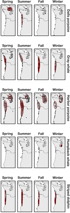
Warlick et al.                                                                                               Cetacean Strandings and Oceanographic Variability

                                            complex ecosystem, improving our understanding of periods of increased strandings
                                            can enhance our knowledge of how these species interact with their environment and
                                            assist conservation and management efforts. This study enhances the utility of stranding
                                            records over time beyond simply reporting trends and has broader applicability to other
                                            geographic regions amid global climate change.
                                            Keywords: cetacean, marine mammal, harbor porpoise, strandings, oceanographic variability, climate variability,
                                            generalized additive model (GAM)

INTRODUCTION                                                                       environmental change are complex, variable, species-dependent,
                                                                                   and often poorly understood, oceanographic features should be
Over the past several decades, marine mammal stranding records                     studied over varying scales (local, continental, and temporal),
have been used as an indicator of ocean and cetacean health                        ecotypes, and cetacean species (Laidre et al., 2008; Evans and
(Gulland and Hall, 2007; Bogomolni et al., 2010; Bossart, 2011).                   Bjørge, 2013; Truchon et al., 2013). Large-scale climate processes
Examining where, when, and how often marine mammals                                such as the El Niño–Southern Oscillation (ENSO) and Pacific
strand can provide insight into ecological behaviors, reproductive                 Decadal Oscillation (PDO) have decade-scale effects on the
success (Norman et al., 2004; Pikesley et al., 2012), health status,               biophysical conditions and food webs of the California Current
the impacts of human activities (Warlick et al., 2018), and                        and Salish Sea ecosystems (Newton, 1995; Mantua and Hare,
local species distribution and abundance (Evans et al., 2005;                      2002; Chavez et al., 2003; Hickey and Banas, 2003). During
MacLeod et al., 2005). The presence of cetaceans is strongly                       the zonal wind phase after the 1970’s, decreased upwelling
influenced by changes in the marine environment via diverse                        and warming waters were observed in the California Current
and dynamic mechanisms, including changes in sea surface                           (McGowan et al., 1998), resulting in a simultaneous decline in
temperature, winds, or large-scale oceanographic oscillations                      primary productivity, zooplankton, pelagic fish, and seabirds.
that can, among other factors, shift the balance of nutrients                      After 2000, sea surface temperatures cooled (Oviatt et al.,
and prey species abundance and distribution (Ballance et al.,                      2015), suggesting that enhanced upwelling and productivity likely
2006). These changes can be amplified through the food web                         occurred, with increased zooplankton abundance noticed since
and may be exacerbated by bioaccumulation of pollutants or                         the late 1990s (Lavaniegos and Ohman, 2007). In recent years, the
toxins from algal blooms, ultimately having noticeable effects                     California Current ecosystem experienced an “extreme marine
on top predators. Here we investigated the possible effects of                     heat wave” that became known as “the Blob”, where above average
oceanographic variability on cetacean strandings by evaluating                     water temperatures persisted from 2014 to 2016, causing a wide
stranding records collected consistently and systematically from                   range of changes in primary productivity, fish spawning, larval
2000 to 2019 in the Pacific Northwest.                                             abundance, and marine wildlife health (Bond et al., 2015; Di
   As top predators, marine mammals may be particularly                            Lorenzo and Mantua, 2016; Auth et al., 2017).
sensitive to alterations in oceanographic and climatic patterns                        These anomalous oceanographic conditions along the
(Moore, 2008; Evans et al., 2010). Recent studies have found                       United States West Coast, along with increasing ocean
correlations between long-term stranding trends and several                        acidification and harmful algal blooms in the Pacific Northwest
indices of climatic variability, demonstrating how strandings                      (Mote and Salathé, 2010; Mauger et al., 2015) can negatively
may be used as bio-indicators of prevailing environmental                          impact marine mammal population dynamics through changes
conditions. Evans et al. (2005) observed that cetacean strandings                  in the abundance and distribution of their prey, among
in southeast Australia exhibited a periodicity coincident with                     other effects (McCabe et al., 2016; Santora et al., 2020). The
regional wind patterns. Factors such as sea ice and the North                      United States Pacific Northwest encompasses coastal, inland, and
Atlantic Oscillation have been found to correlate with strandings                  estuarine waters extending from northern California through
and mortality of certain pinniped and cetacean species in the Gulf                 British Columbia, including the Salish Sea and the mouth of
of St. Lawrence, Canada (Johnston et al., 2012; Soulen et al., 2013;               the Columbia River. It is an ecosystem that contains important
Truchon et al., 2013). El Niño conditions have corresponded with                   feeding and breeding habitat for numerous marine mammal
increased California sea lion (Zalophus californianus) strandings                  species in the eastern north Pacific and beyond, including gray
and fisheries interactions along the California coast (Keledjian                   whales (Eschrichtius robustus), humpback whales (Megaptera
and Mesnick, 2013). Berini et al. (2015) noted that pygmy sperm                    novaeangliae), endangered southern resident killer whales
whale (Kogia breviceps) strandings in the southeast United States                  (Orcinus orca), and numerous smaller odontocete species
were positively correlated with sea surface temperatures, wind,                    (Calambokidis et al., 2015; Norman et al., 2018).
and barometric pressure.                                                               Studying the mechanisms that give rise to patterns in marine
   Environmental changes are acknowledged to be occurring                          mammal strandings is complicated by numerous factors, one of
on a global scale (IPCC, 2014), though the local realization                       which is that observed strandings are not necessarily a direct
of these changes is patchy and difficult to predict due to                         reflection of changes in actual mortality rates. While actual
ecosystem complexity and spatial heterogeneity (Moore, 2008;                       mortality rates may be changing over a given time period,
Evans and Bjørge, 2013; Jacox et al., 2016). Because responses to                  observed changes in stranding cases may be more a product

Frontiers in Marine Science | www.frontiersin.org                              2                                        March 2022 | Volume 9 | Article 758812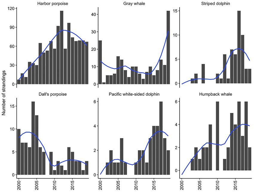
Warlick et al.                                                                                      Cetacean Strandings and Oceanographic Variability

of seasonal changes in abundance and distribution (e.g., for               incidents of HI could hypothetically be exacerbated by certain
migratory species such as large whales), interannual changes               oceanographic conditions as has been documented for pinnipeds
in abundance and distribution (e.g., population recovery or                (Keledjian and Mesnick, 2013).
recolonization), changes in reporting protocols and capacity                  Approximately 15 percent of all cases during the study period
(e.g., less reporting in winter or inaccessible coastal areas),            were observed in a state of advanced decomposition and 6 percent
and changes in oceanographic conditions or the cause of                    of cases were missing this information. These cases were retained
strandings that may affect the likelihood of an individual                 to maximize sample size and document total strandings over
washing onshore versus sinking at sea (Moore et al., 2020).                the study period, though this could introduce a small degree of
Despite these caveats, examining changes in strandings over                bias in our results with respect to the seasonality of strandings
time provides important information for monitoring cetacean                (largely for harbor porpoise and gray whales, as they comprise
populations, tracking distribution or abundance trends, and                approximately 50% and 25% of these more decomposed or
examining emerging health or disease conditions, particularly              unknown decomposition state cases, respectively.
in light of recently documented changes in oceanographic                      Stranding records were aggregated by year, month, geographic
conditions on both local and regional scales (Pierce et al., 2007;         state (OR/WA), and stranding region (inland Washington
Truchon et al., 2013; Sprogis et al., 2017). The goals of this study       waters east of the western entrance to the Strait of Juan de
were to compare recent cetacean stranding patterns in the Pacific          Fuca versus the outer coast), similar to Warlick et al. (2018).
Northwest to those previously reported for 1930–2002 (Norman               This study region has a diverse coastline ranging from rocky
et al., 2004); examine strandings as a proxy for the changing              intertidal zones to estuarine embayments and variable degrees of
prevalence of cetacean species within certain geographic areas;            public access and development (e.g., residential and commercial
and to investigate possible relationships between spatiotemporal           districts, ports, fishing activity, shipping and ferry channels,
variation in cetacean strandings and oceanographic conditions.             and ecotourism). Seasons were defined as Spring: March-
Understanding the complex mechanisms that affect marine                    May; Summer: June-August; Fall: September-November; Winter:
mammal strandings with respect to changes in environmental                 December-February. Strandings for all species were qualitatively
conditions can provide useful insights into the health of cetacean         summarized, though only five focal species were explored using
populations and has broad applicability to other geographic                statistical analyses.
regions amid global climate change.
                                                                           Environmental Data
                                                                           Local Oceanographic Conditions
MATERIALS AND METHODS                                                      Variables representing local oceanographic conditions were
                                                                           obtained from satellite data and reanalysis products using
Study Area and Stranding Data                                              NOAA data server ERDDAP (Simons, 2019), and Copernicus
We compiled all available Level A records of cetacean                      Marine Environment Monitoring Service, spanning an area
strandings (2000–2019) that are maintained by the U. S.                    off the coasts of Oregon and Washington (42.0◦ N/123.0◦ W
NOAA Fisheries and its stranding response network members                  to 48.3◦ N/127.3◦ W; Figure 1). The spatio-temporal scope for
in Oregon and Washington. Strandings are detected by                       environmental covariates was selected with the aim of being
dedicated beach survey efforts (Huggins et al., 2015a) or                  localized and relevant to the cetaceans and yet large enough to
reports from the public or field researchers, which are then               encompass likely foraging habitat and smooth over fine-scale
verified by stranding network partners. Stranding reports                  anomalies. Sea surface temperature (SST, ◦ C) and chlorophyll
are submitted regularly to NOAA’s national stranding                       concentration were obtained from Aqua MODIS satellite sensor
database by network members and include basic data such                    data (NOAA Southwest Fisheries Science Center Environmental
as observation date, stranding location, and when determinable,            Research Division (SWFSC ERD), 2019) and aggregated for
age class, sex, status (dead or alive), species, evidence of               monthly values for each year 2000–2019 across the study region.
injury or human interaction (HI), and level of postmortem                  Data on mixed layer depth, sea surface height (an atmospheric
condition. Level A data do not include the cause of the                    index of climate that represents the average of variations in
stranding event or mortality. Reports containing ambiguous                 the highs and lows of the ocean’s surface; Oviatt et al., 2015),
species identification, regardless of source, were included in             and meridional (north-south longitudinally-directed) and zonal
one of several ‘Unknown’ categories based on the level of                  (east-west latitudinally directed) winds were derived from the
information known.                                                         ARMOR3D L4 reanalysis data product (Mertz et al., 2019) and
   With the exception of live free-swimming entangled animals,             also aggregated at the monthly level. Changes in SST can be
cases noted as involving human interactions were included in the           indicative of El Niño conditions that can also be associated with
total stranding counts reported in this study. Documented HI               changing prey availability. Chlorophyll, mixed layer depth, and
findings within this dataset included those that were unrelated            indices of wind velocity can be measures of the degree and
to any apparent cause of stranding or mortality (e.g., healed              strength of upwelling and primary production, which both affect
entanglement wound), and determination of HI can be hindered               the timing, amount, type, and diversity of available copepods and,
by decomposition or inability to conduct a thorough external               after a certain amount of lag time, forage fish and other prey items
and internal examination. Though the inclusion of cases where              (Peterson and Keister, 2003; Tian et al., 2004; Ainsworth et al.,
HI likely contributed to the stranding could complicate the                2011; Oviatt et al., 2015; Santora et al., 2017). Sea surface height
interpretation of correlations with environmental variables,               can be a measure of eddy strength, general ocean circulation,

Frontiers in Marine Science | www.frontiersin.org                      3                                       March 2022 | Volume 9 | Article 758812
Warlick et al. Cetacean Strandings and Oceanographic Variability
we hypothesized that changes in these dynamic landscape
features could affect the distribution, abundance, and, availability
of prey species or other factors that could directly affect survival,
reproduction, or the probability of individuals washing onshore.
Statistical Analysis
To examine seasonal and interannual patterns in stranding cases
and whether variability in monthly strandings correlated with
oceanographic conditions, we fit generalized additive models
(GAM; Hastie and Tibshirani, 1990),
ys,m,t ∼ Poisson(µs,m,t ) (1)
log(µs,m,t ) = β0s + f1 (Yeart ) + f2 (Monthm ) + fb (xm,t )
(2)
where the number of stranding cases y for each species s in each
month m and year t were assumed to be Poisson-distributed with
the natural log of mean monthly cases µs,m,t being a function
of intercept β0 and smooth functions f for year, month, and b
number of environmental covariates x (Equations 1-2).
To account for the fact that the larger migratory species are
only seasonally present in the study region, additional models
examining strandings and environmental covariates at the annual
level were conducted for gray and humpback whales, though only
a limited number of covariates could be included simultaneously
due to the smaller sample size. Additionally, models for harbor
porpoises were conducted at the regional level (e.g., inland versus
outer coast strandings) to account for potential differences in
habitat use among the different ecosystems and harbor porpoise
FIGURE 1 | Map of the study area indicating Oregon and Washington in populations. Results, however, are largely reported for aggregate
darker gray with the black rectangle representing the spatial extent from which harbor porpoise strandings.
localized and satellite data for oceanographic covariates were gathered. The GAM framework enables the examination of potentially
non-linear relationships between strandings and oceanographic
storm activity, and changes in atmospheric pressure, which can conditions (e.g., if there was an ideal temperature range for a
all alter the aforementioned prey indices. given species below and/or above which strandings increased).
The effective degrees of freedom (edf) is a measure of the
Large-Scale Oceanographic Oscillations degree of ‘wiggliness’ in that non-linear relationship, where
Variables used to assess the effect of large-scale, climatic factors an edf close to 1.0 would indicate that the relationship is
on strandings included the Multivariate El Niño Southern in fact linear (values < 1.0 indicate shrinkage due to the
Oscillation index (MEI), the PDO, and the North Pacific null space penalization). The GAMs were fit with a Poisson
Gyre Oscillation (NPGO), all of which were obtained from distribution and a cyclic cubic spline to estimate the effect
the California Current Integrated Ecosystem Assessment (IEA) of month and a thin plate spline for all other variables
project data portal at the monthly level (NOAA Integrated using restricted maximum likelihood (REML) using the mgcv
Ecosystem Assessment (IEA), 2019). The MEI describes El package (Wood, 2011) in the R statistical programming language
Niño conditions since it combines six meteorological measures (R Development Core Team, 2019).
over portions of the Pacific Ocean (Wolter and Timlin, Variable selection with respect to oceanographic covariates
1993). Large positive MEI values indicate the occurrence was conducted using null space penalization and removing
of El Niño conditions, while large negative MEI values variables with an edf less than 0.4. The final model was
indicate La Niña conditions. The PDO represents a recurring selected by minimizing the Akaike’s Information Criterion (AIC)
pattern of climate variability (Mantua and Hare, 2002) with (Akaike, 1973) in conjunction with biological relevance. Because
historical records strongly suggesting an association with many of the oceanographic variables are inter-related, we tested
salmon production (Beamish et al., 1999; Hare et al., 1999) for collinearity between variables using a Pearson’s correlation
and zooplankton production in the eastern North Pacific coefficient and did not include highly correlated variables in
Ocean (Francis et al., 2003). The NPGO is largely associated the same models. The best models that included oceanographic
with variation in sea surface height, salinity, and nutrient variables were compared to null models and models with only
concentrations (Di Lorenzo et al., 2008). These local and basin- year and month effects. P-values of smooth terms are largely
scale variables were included in this exploratory analysis because approximate due to the challenge of comparing degrees of
Frontiers in Marine Science | www.frontiersin.org 4 March 2022 | Volume 9 | Article 758812Warlick et al. Cetacean Strandings and Oceanographic Variability freedom between GAM models (Wood, 2011). Environmental be limited due to lack of this information for most strandings. conditions were considered in both real-time and one- to This study also has the added complexity of not being able three-month lags. Longer lag times that may be ecologically to define the relationship between environmental conditions realistic were not explored due to the constraints of examining and health of the animal, nor how the environmental indices a reasonable number of possible models. To qualitatively relate to habitat use, distribution patterns, or the likelihood of a examine spatio-temporal stranding patterns across seasons and carcass washing ashore. regions, hotspot maps were generated with a kernel density estimation (Gatrell et al., 1996) (‘geom_density2d’ function in the ggplot2 R package). RESULTS Methodological Limitations Over the study period (2000–2019), 1,819 cetacean strandings All stranded animals, regardless of cause of death, were included were recorded in Oregon (n = 613) and Washington (n = 1,206) in the analysis, though the cause of death was not included in (Tables 1, 2) across 26 species and a hybrid combination GAM models. Although it could be illuminating to formally (Phocoena phocoena/Phocoenoides dalli). The number of include cause of death in the analysis, the sample size would strandings in Washington was further broken down by outer TABLE 1 | Cetacean stranding cases in Oregon (OR) and Washington (WA) from 2000 to 2019 by species and sex. Species Total OR WA Inland Outer Male Female Undetermined Balaenopteridae Balaenoptera musculus 1 1 0 0 0 1 0 0 Balaenoptera physalus 13 2 11 8 3 9 2 2 Balaenoptera borealis 1 0 1 1 0 1 0 0 Balaenoptera edeni 2 0 2 2 0 2 0 0 Balaenoptera acutorostrata 6 3 3 2 1 2 4 0 Megaptera novaeangliae 47 20 27 6 21 18 16 13 Eschrichtiidae Eschrichtius robustus 208 61 147 41 106 78 69 61 Physeteridae Physeter macrocephalus 24 15 9 0 9 7 8 9 Kogia breviceps 7 4 3 0 3 2 3 2 Ziphiidae Berardius bairdii 5 2 3 0 3 1 3 1 Mesoplodon carlhubbsi 1 0 1 0 1 0 1 0 Mesoplodon densirostris 1 0 1 0 1 0 1 0 Mesoplodon stejnegeri 6 3 3 0 3 1 4 1 Ziphius cavirostris 9 9 0 0 0 8 0 1 Delphinidae Delphinus capensis 9 2 7 2 5 7 2 0 Delphinus delphis 16 12 4 0 4 6 9 1 Globicephala macrorhynchus 2 1 1 0 1 0 1 1 Grampus griseus 7 6 1 1 0 5 2 0 Sagmatias obliquidens 37 26 11 1 10 14 16 7 Lissodelphis borealis 11 8 3 0 3 5 4 2 Orcinus orca 19 4 15 9 6 5 10 4 Stenella attenuata 1 1 0 0 0 0 1 0 Stenella coeruleoalba 61 48 13 0 13 33 19 9 Tursiops truncatus 4 1 3 3 0 1 3 0 Phocoenidae Phocoena phocoena 1136 322 814 437 377 414 366 356 Phocoenoides dalli 103 17 86 58 28 40 18 45 Phocoenidae hybrid 2 0 2 2 0 1 1 0 Unidentified Species Unidentified 80 45 35 18 17 4 2 74 Total 1819 613 1206 591 615 665 565 589 Inland and Outer refer to inland waters and outer coast of Washington State, respectively. Frontiers in Marine Science | www.frontiersin.org 5 March 2022 | Volume 9 | Article 758812
Warlick et al.                                                                                                    Cetacean Strandings and Oceanographic Variability

TABLE 2 | Cetacean strandings in Oregon/Washington by species and year, 2000–2019.

Species               2000 2001 2002 2003 2004 2005 2006 2007 2008 2009 2010 2011                    2012   2013 2014 2015 2016 2017 2018 2019               Total

Balaenopterid
Balaenoptera           0     0     0      0         0    0     0     0     0     0        0     0     0      0      0     1/0      0      0     0      0      1/0
musculus
Balaenoptera           0     0    1/3     0         0    0     0/2   0     0     1/1     0/1   0/1    0     0/2     0     0        0     0/1    0      0      2/11
physalus
Balaenoptera           0     0     0     0/1        0    0     0     0     0     0        0     0     0      0      0     0        0      0     0      0      0/1
borealis
Balaenoptera edeni     0     0     0      0         0    0     0     0     0     0       0/2    0     0      0      0     0        0      0     0      0      0/2
Balaenoptera           0     0     0     1/0    1/0      0     0/1   0     0     0       1/0    0     0      0     0/1    0        0     0/1    0      0      3/3
acutorostrata
Megaptera              0     0     0     1/0    1/1     1/0    1/1   2/0   0/4   0       6/0    0    1/0    0/2    2/3    1/3     3/3    0/3   0/6    1/1    20/27
novaeangliae
Eschrichtiidae
Eschrichtius          2/23 0/1    3/2    2/3    3/2     4/11   4/9   4/4   2/2   3/7     3/7   2/4   0/3    3/4    5/5    2/3     4/4    7/8   1/10 7/35    61/147
robustus
Physeteridae
Physeter              0/1    0    2/2    1/0    1/0     1/0    0     2/1   1/2   1/0     1/0    0    0/2    1/0    1/0     0      0/1    2/0   1/1    0/0    15/10
macrocephalus
Kogia breviceps        0     0     0      0         0   0/2    1/0   0     0     0        0     0     0      0      0     0       1/0    1/0    0     1/0     4/2
Ziphiidae
Berardius bairdii      0     0     0     1/1        0    0     0     0     0     0       1/0    0     0      0      0     0/1      0     0/1    0      0      2/3
Mesoplodon             0     0     0      0         0    0     0     0     0     0       0/1    0     0      0      0     0        0      0     0      0      0/1
carlhubbsi
Mesoplodon             0     0     0      0         0    0     0     0     0     0        0     0     0      0      0     0       0/1     0     0      0      0/1
densirostris
Mesoplodon             0    1/1    0     1/0        0    0     0     0     0     0        0     0     0      0      0     1/1      0      0    0/1     0      3/3
stejnegeri
Ziphius cavirostris    0    1/0   1/0     0         0   1/0    2/0   1/0   2/0   0        0     0     0     1/0     0     0        0      0     0      0      9/0
Delphinidae
Delphinus capensis     0     0     0      0         0    0     0     0     0     0       0/1    0    0/1     0      0     0/1     1/1    1/1   0/1    0/1     2/7
Delphinus delphis      0     0     0      0         0    0     1/1   1/0   0     1/0      0    1/0    0     2/0    1/2    2/0      0     1/0   2/1     0      12/4
Globicephala           0     0    0/1     0         0    0     0     1/0   0     0        0     0     0      0      0     0        0      0     0      0      1/1
macrorhynchus
Grampus griseus       1/0    0     0      0         0    0     0     0     0     0        0     0     0     4/0    1/0    0/1      0      0     0      0      6/1
Lissodelphis           0     0     0     0/1    1/0      0     0     0/1   1/0   0        0     0    1/0     0      0     1/0     1/1    1/0   1/0    1/0     8/3
borealis
Orcinus orca          1/0    0    0/3     0     1/0      0     0     0/1   0/1   0       0/2   1/1   0/1    0/1     0     0/1     0/2    1/0   0/2    0/0     4/15
Sagmatias              0     0    0/1    2/0    1/0     0/1    2/1   1/0   0     0       1/0   2/0   2/0    1/0    2/1    3/1     2/2    4/2   2/1    1/1    26/11
obliquidens
Stenella attenuata     0     0     0      0         0    0     0     0     0     0        0     0     0      0     1/0    0        0      0     0     0/0     1/0
Stenella               0     0     0     1/0    2/0      0     4/0   0     0     0       2/0   0/1   4/2    1/0    5/2    5/1    10/5 10/0     2/1    2/1    48/13
coeruleoalba
Tursiops truncatus     0     0     0      0     0/1      0     0     0     0     0       0/1   0/1   1/0     0      0     0        0      0     0     0/0     1/3
Phocoenidae
Phocoena              1/6 2/17    2/9    9/26 21/12 6/24 15/50 21/29 20/33 22/46 16/40 25/67 27/89 18/38 22/75 19/56 18/50 18/51 23/46 17/50 322/814
phocoena
Phocoenoides dalli 0/10 1/6       0/7    1/5    1/15 2/11      1/5   2/3   0     1/4     0/1   0/3   1/1    0/1    3/3    2/3     1/2    1/2   0/1    0/3    17/86
Phocoenidae            0     0     0      0         0    0     0     0/1   0     0        0    0/1    0      0      0     0        0      0     0     0/0     0/2
hybrid
Unidentified
Species
Unidentified          4/2   1/1   2/1    3/2    4/5     0/2    4/1   4/3   3/1   4/1     0/2   3/2   0/1    1/1    1/1    2/2     4/0    3/3   1/4    1/0    45/35
Total                 9/42 6/26 11/29 23/39 37/36 15/51 35/71 39/43 29/43 33/59 31/58 34/81 37/100 32/49 44/93 39/74 45/72 50/73 33/75 31/92 613/1206

coast (n = 615) and inland waters (n = 591). Nearly all                                over the study period for harbor porpoises, gray whales, and
cases (96%) were identified to species level. The five most                            Dall’s porpoise were 56, 10.4, and 5.5 cases per year, respectively,
commonly stranded species were harbor porpoise, gray whale,                            and combined represented approximately 79% of total strandings
Dall’s porpoise (Phocoenoides dalli), striped dolphin (Stenella                        (Table 1). Striped dolphins were the most commonly stranded
coeruleoalba), and humpback whales. Mean annual strandings                             delphinid species (annual mean = 4.7; 3% of all total strandings),

Frontiers in Marine Science | www.frontiersin.org                                6                                             March 2022 | Volume 9 | Article 758812
Warlick et al. Cetacean Strandings and Oceanographic Variability
with 79% of reports in Oregon. Mean annual strandings for in the fall and winter (mean of 12–15 per year per season)
humpback whales, 3 per year, represented 2.5% of total stranding compared with the spring and summer (mean of 28–36 per
cases. Though sex could not be determined for approximately year per season). The effect of month in GAMs models was
one-third of strandings, there was no significant difference significant for four of the five focal species, indicating seasonal
between the number of males and females over the study period peaks in strandings between June-August for harbor porpoises
for any of the five most commonly stranded species. Greater and humpback whales, and an earlier peak in May for Dall’s
than one-third (n = 437; 38%) of all harbor porpoise strandings porpoises and gray whales, though these patterns depended on
were reported in the inland waters of Washington State, 33% the region (Figure 3).
(n = 377) along Washington’s outer coast, and the remainder
(n = 322) in Oregon.
Spatial Distribution
Overall, the number of strandings reported in inland Washington
Temporal Distribution waters was higher than that reported along the coasts, though
Over the study period, combined strandings have increased over this was largely driven by harbor porpoise strandings. Other
time, though this pattern has varied across species (Table 2). frequently stranded species exhibited different spatial trends, with
Harbor porpoise strandings increased throughout the 2000s and a higher number of striped dolphins stranding in Oregon, Dall’s
then peaked in 2012. Reports of stranded humpback whales and porpoise strandings clustering in inland Washington waters, and
striped dolphins in the study area have increased since 2003 gray whales along the outer Washington coast (Figure 4). At
while Dall’s porpoise strandings have decreased and gray whale the seasonal level, gray and humpback whale strandings were
strandings have fluctuated interannually with little apparent concentrated further south in Oregon on the outer coast during
directional trend during the study period (Figure 2). fall compared with other months when more strandings occurred
Overall, there were notable differences in the number of in Washington (Figure 4). For harbor porpoises, cases were more
strandings per season, with fewer strandings across all species frequently reported on the outer coast at their peak in the summer
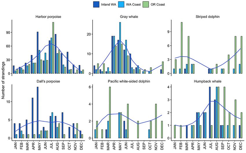
FIGURE 2 | Total annual stranding cases and smoothed loess line for the six most commonly stranding species from 2000 to 2019 in Oregon and Washington. Note
difference in scale of y-axes.
Frontiers in Marine Science | www.frontiersin.org 7 March 2022 | Volume 9 | Article 758812Warlick et al. Cetacean Strandings and Oceanographic Variability
FIGURE 3 | Total monthly regional stranding cases (bars) and smoothed loess line for total combined cases across regions (blue) for the six most commonly
stranding species from 2000 to 2019 in Oregon and inland and coastal Washington.
compared to being relatively more concentrated in inland waters These environmental indices explained 71% of deviance for outer
the rest of the year. coast strandings, but only 42% of deviance for strandings that
occurred in inland waters.
Oceanographic Conditions Monthly gray whale strandings were best explained by a model
To examine the effect of ocean conditions and interannual and that included smooth terms for year (edf = 5.9, p < 0.01),
seasonal patterns of stranding cases, GAMs were fit for the five month (edf = 5.4, p < 0.01), sea surface temperature (edf = 1.0,
most commonly stranded focal species: harbor porpoise, gray and p < 0.1), chlorophyll (edf = 3.3, p < 0.05), and one-month
humpback whales, Dall’s porpoise, and striped dolphin. For all lagged PDO (edf = 2.2, p < 0.01). This model would predict
five focal species, including environmental covariates improved decreased strandings in conditions with lower temperatures,
model fit as evidenced by lower AIC values and higher deviance higher chlorophyll concentration, and negative phase PDO, with
explained (Table 3). a seasonal peak in May (Figure 5). The addition of environmental
For harbor porpoise, the best model of aggregate region- covariates to the model contributed less to model fit compared to
wide strandings included smooth effects of year (edf = 5.1, the other species (56% versus 60% deviance explained, Table 3).
p < 0.01), month (edf = 5.6, p < 0.01), chlorophyll (edf = 4.7, At the annual level, the best-fit model included smooth terms for
p < 0.01), and one-month lagged PDO (edf = 1.1, p < 0.1) MEI (edf = 6.5, p < 0.01) and year (edf = 1.9, p < 0.01), which
and mixed layer depth (edf = 5.8, p < 0.01) (Figure 5). explained 58% of deviance. Gray whale strandings were notably
This model would predict increased strandings in late summer higher in 2000 and 2019 compared to all the years in between.
and under conditions with lower chlorophyll concentrations, Striped dolphin strandings have exhibited an increasing trend
smaller mixed layer depths, and positive phase PDO. Though (edf = 1.1, p < 0.01) and the best-fit model included smooth
not included in the best-fit model due to being correlated effects of month (edf = 3.2, p < 0.01), sea surface height (edf = 3.9,
with chlorophyll concentration, meridional and zonal wind p < 0.01), chlorophyll (edf = 1.7, p < 0.01), and lagged sea
velocities were also strong predictors of monthly stranding surface temperature (edf = 1.4, p < 0.1) (Figure 3). This model
cases. This best model with environmental covariates explained would predict a higher number of cases in late winter-early spring
69% deviance, higher than the other focal species most or during months with increased sea surface height and lower
likely due to the higher sample size rather than a tighter temperatures and chlorophyll concentrations (Figure 5). This
association between strandings and oceanographic conditions. model with covariates explained more of the deviance (49%) and
Frontiers in Marine Science | www.frontiersin.org 8 March 2022 | Volume 9 | Article 758812Warlick et al. Cetacean Strandings and Oceanographic Variability
TABLE 3 | Best models for monthly stranding counts for harbor porpoise, gray
whale, Dall’s porpoise, and striped dolphin over the study period compared to null
models and models without environmental covariates, including the effective
degrees of freedom (edf) and p-values for smooth effect terms, Akaike Information
Criterion (AIC) values, and deviance explained.
Species Model AIC δAIC Dev. expl
Harbor porpoise ∼1 (null) 1892.3 792.1 –
∼ s(year) + s(month) 1139.7 39.5 63%
∼ s(year) + s(month)+ 1100.1 0.0 69%
s(mld, lag) + s(chl) +
s(PDO, lag)
Gray whale ∼1 (null) 766.2 273.2 –
∼ s(year) + s(month) 499.2 6.3 56%
∼ s(year) + s(month) + 492.9 0.0 60%
s(sst) + s(chl) + s(PDO,
lag)
Striped dolphin ∼1 (null) 339.8 109.6 –
∼ s(year) + s(month) 261.0 30.9 38%
∼ s(year) + s(month) + 230.2 0.0 49%
s(SST, lag) + s(chl) +
s(ssh)
Dall’s porpoise ∼1 (null) 426.7 39.5 –
∼ s(year) + s(month) 393.1 5.8 19%
∼ s(year) + s(month) + 387.2 0.0 22%
s(sst) + s(PDO, lag)
Humpback whale ∼1 (null) 255.2 26.8 –
∼ s(year) + s(month) 231.1 2.7 19%
∼ s(year) + s(month) + 228.4 0.0 23%
s(sst, lag) + s(chl, lag)
Smooth terms with p < 0.05 in the best models are indicated in bold. Environmental
covariates in best-fit models include sea surface temperature (sst), sea surface
height (ssh), Pacific Decadal Oscillation (PDO), mixed layer depth (mld), and
chlorophyll concentration (chl) in real time and one-month lags.
had a lower AIC value compared to the model with only an
interannual effect (38% deviance, Table 3).
In the case of Dall’s porpoise strandings, strandings have
decreased over the study period (edf = 1.0, p < 0.01) and
the best model included smooth effects of month (edf = 1.5,
p < 0.05) and lagged PDO (edf = 3.7, p < 0.05), and linear
effects of SST (edf = 1.0, p < 0.5) (Figure 5). This best
model would predict peak seasonal strandings during May-June,
increased strandings with warmer temperatures and decreased
strandings with negative-phase PDO values (Figure 5). Including
environmental covariates improved model fit but the model
overall has low explained deviance at 22% (Table 3).
Humpback whale strandings have increased in recent years.
The best model for this species included a nearly linear effect of
year (edf = 1.2, p < 0.05) and lagged SST (edf = 0.7, p < 0.05),
and smooth effects of month (edf = 1.8, p < 0.05) and lagged
chlorophyll (edf = 1.8, p < 0.05). This best model would predict
peak strandings in summer and lower strandings in months
FIGURE 4 | Seasonal distribution of stranding cases for each of the five most after higher chlorophyll concentrations and lower temperatures
commonly stranding species. Kernel density estimation is calculated for each (Figure 5). Including environmental covariates only marginally
season and species separately, therefore contour lines are intended to show improved model fit (23% deviance explained) over the model
the spatial density of strandings in each panel relative to itself, not compared
to others.
with just annual and monthly effects (19% deviance explained)
(Table 3). However, the best model fit to annual strandings
Frontiers in Marine Science | www.frontiersin.org 9 March 2022 | Volume 9 | Article 758812Warlick et al. Cetacean Strandings and Oceanographic Variability FIGURE 5 | Estimated smooth effects of environmental variables for best-fit models of monthly stranding cases for each of five focal species, with effective degrees of freedom (edf), confidence intervals, and p-values indicated. Frontiers in Marine Science | www.frontiersin.org 10 March 2022 | Volume 9 | Article 758812
Warlick et al.                                                                                       Cetacean Strandings and Oceanographic Variability

included smooth terms for SST (edf = 0.8, p < 0.01) and                     Huggins et al., 2015b), likely reflects a greater presence of
chlorophyll (edf = 2.1, p < 0.05) and explained 57% of deviance.            this species in inland Washington waters (i.e., Puget Sound),
                                                                            its seasonal distribution, and the growth of coastal and
                                                                            inland populations over this time period through mediation of
DISCUSSION                                                                  anthropogenic factors such as fishery interactions and pollutants
                                                                            (Hanson, 2007; Smultea et al., 2015; Evenson et al., 2016; Jefferson
This study examined spatial, annual, and seasonal trends in                 et al., 2016). Similar increases in population growth were
cetacean stranding cases in the Pacific Northwest region of                 documented in California harbor porpoise stocks after protection
the United States with the aim of comparing these results                   from gill net fishery bycatch was implemented (Forney et al.,
to previously identified stranding patterns and to examine                  2020). Other factors potentially contributing to the increased
whether some variability in stranding cases can be explained                harbor porpoise reports include changes in stranding response
by oceanographic conditions over the study period. Stranding                effort and the distribution and impact of human activities, which
reports for many species increased since 2000 and are notably               could similarly affect all species in this study.
higher per year than numbers reported by Norman et al. (2004).                 While gray whale strandings were highly variable by year,
Incorporating environmental variables in GAMs improved                      the high number in 2000 and 2019 reflected larger trends in
model fit for all of the five most commonly stranded species                gray whale mortality along their entire range from Mexico
(though some more notably than others), indicating that some                to the Arctic. Gray whales have experienced two Unusual
variability in stranding cases can be explained by oceanographic            Mortality Events (UMEs) during the study period that remain
conditions. The GAM framework is beneficial in this context                 undetermined: one occurring from 1999 to 2000 (Moore et al.,
because it allows for the estimation of non-linear effects of               2001; Gulland et al., 2005) and one beginning in 2019 and
environmental covariates, which may most accurately reflect                 extending throughout 2021 (NOAA Fisheries, 2021).
how species likely have optimum niche ranges for certain                       The number of Dall’s porpoise strandings significantly
oceanographic conditions or ecosystem states that affect prey               decreased until 2011, which could have been a change
availability, foraging behavior, the prevalence of storms, or even          in population size or distribution. Anecdotal evidence has
disease. Our results indicate that it may be possible to identify           demonstrated fewer live sightings throughout inland Washington
relationships between oceanographic variability and patterns in             waters by individuals spending a large portion of their time
strandings for some species. However, we cannot definitively                on the water. However, recent abundance estimates have
identify the causal mechanisms behind these correlations with               not been conducted to confirm this. Notable increases in
this framework, particularly due to our exploration of relatively           stranding cases occurred for striped dolphins and humpback
short temporal lag times and the noise that exists in stranding             whales. Though striped dolphin abundance trends have varied
patterns due to unmodeled changes in localized abundance and                interannually from 1991 to 2014 (Becker et al., 2012; Barlow,
distribution of each species, which would be better suited for              2016), strandings significantly increased over the last 20 years in
more focused future studies.                                                the Pacific Northwest compared to numbers previously reported
                                                                            (Norman et al., 2004), with a steep increase beginning in
Interannual Variability                                                     2010–2011 (Figure 2). An increase in the number of stranded
Our results suggest that the interannual variability of marine              humpback whales occurred over the study period, with a
mammal stranding events over a 20-year period is associated                 particular uptick starting in 2008, likely reflecting increases
with both regional and basin-scale oceanographic conditions,                in the population of the California-Oregon-Washington stock
though patterns and correlations differ for each of the five                over the past 20–30 years, and a shift in habitat use such
most commonly stranded species (Table 2). The smaller number                that more animals are now occupying northeastern Pacific
of monthly stranding cases for many species makes the                       Ocean waters (Barlow et al., 2011; Calambokidis et al., 2017;
identification of these correlations impossible for all species that        Calambokidis and Barlow, 2020).
stranded over the study period.
   Long-term increases in the number of reported strandings                 Spatio-Temporal Trends
may result from changes in reporting effort due to increasing               Spatio-temporal trends in stranding cases likely largely reflect
coastal activities, human habitation, public interest in marine             the seasonal distribution and prevalence of each species based
mammals, as well as changes in the abundance and distribution               on life history characteristics such as calving requirements and
of the species themselves (Huggins et al., 2015a; Segawa and                migratory and foraging behavior. However, because such a large
Kemper, 2015; Prado et al., 2016; Pitchford et al., 2018;                   proportion of cases are reported by the public, strandings are
Warlick et al., 2018). Harbor porpoise are a good example of                more likely to be detected and reported from more densely
possible influences of changes in reporting effort and changes in           populated areas with accessible beaches (inland waters) in
abundance on the number of observed strandings.                             warmer, drier, beach-going months (summer).
   An increasing trend in harbor porpoise strandings was                       The majority (72%) of harbor porpoise strandings occurred
documented until 2011–2012, at which time a plateau or decline              in WA (particularly inland waters) and peaked seasonally in
in stranding reports was observed, continuing through 2019                  August, with a lesser peak in late spring, in contrast to a
(Figure 2). This notable rise in stranding cases over the study             pattern of maximum strandings in summer and fall previously
period, particularly in inland waters (Norman et al., 2004;                 reported (Norman et al., 2004). Though cause of stranding

Frontiers in Marine Science | www.frontiersin.org                      11                                       March 2022 | Volume 9 | Article 758812
Warlick et al. Cetacean Strandings and Oceanographic Variability
and mortality is generally not discussed here, a noteworthy explained by an overall decrease in the Dall’s porpoise population
finding was that most of the fishery interactions documented in abundance in this region, while a simultaneous increase in
harbor porpoises were recorded in the fall months (September- harbor porpoise abundance occurred (Evenson et al., 2016).
November) and were spatially concentrated along the western Shifts in prey abundance or distribution may help explain
shoreline of mid- to southern Puget Sound. These cases were this shift in Dall’s abundance, and thus strandings, but further
confirmed with detailed examinations and elimination of other investigation is warranted.
major contributory causes of death (Huggins et al., 2015b; NOAA Though striped dolphins have a widespread offshore
Fisheries, unpublished data). However, it is important to interpret distribution (Mangels and Gerrodette, 1994; Forney et al., 1995),
findings of HI on stranded animals with extreme caution, as little is known about the seasonality of their distribution and
strandings demonstrating signs of HI do not necessarily indicate movement to contextualize our finding that fewer cases are
that the injury or condition was the cause of stranding (e.g., could reported in the summer compared to the fall and winter. Their
include cases with previously healed entanglement wounds) and abundance may vary from year to year and may be affected by
it is often impossible to ascertain cause of death with certainty. oceanographic conditions, but long-term trends have not been
Though many commercial and tribal salmon fisheries are highly identified (Becker et al., 2012; Barlow, 2016). Striped dolphins
regulated (Washington Department of Fish and Wildlife, 2020), are rarely observed during coastwide cetacean surveys in the
interactions with other net-based fisheries may still exist on a waters of Washington and Oregon and are thus considered a low
smaller scale and may be underreported. HI cases are likely abundance species in the region, but may seasonally shift into
underestimated because evidence of human-caused injury and the area outside of the survey season (i.e., during winter) or due
mortality can go undetected in strandings that are not necropsied to anomalous warm waters. For example, the species may have
or are in an advanced state of decomposition. undergone a temporary northern range expansion due to warm
The proportion of harbor porpoise strandings occurring in water incursions from events such as “the Blob” (Becker et al.,
inland WA versus the outer coast (55 vs. 45%, respectively) has 2012; Bond et al., 2015; Barlow, 2016). Of the striped dolphins
remained relatively similar since those reported in Norman et al. stranded in WA and OR, most had neurological disease and
(2004), and have followed similar peaks and troughs over the last a disproportionate number of them live stranded, suggesting
20 years. However, one notable difference is the seasonal peak that this increase of strandings may be disease related, with
in regional strandings. Prior to 2000, strandings peaked in late greater representation in Washington compared to prior years
summer and early fall (Norman et al., 2004). In this study, we (Norman et al., 2004).
found that strandings increased in May (particularly for the outer No range expansions were noted for the other species of
WA coast) and peaked in July (for inland WA and OR coast) cetaceans in this study; however, information on spatial and
(Figure 3). This pattern can be validated by the recent higher seasonal population trends are incomplete or lacking for many
observed live porpoise numbers in spring. The cause of this species (Carretta et al., 2020). Strandings of some species showed
seasonal shift and the general rise in sightings remains unknown seasonal trends that likely reflect seasonal distribution, but these
(Jefferson et al., 2016). Harbor porpoises are the most commonly patterns may also be due to increased summer stranding response
stranded cetacean in the Pacific Northwest, as also noted in the effort and public interest. On the other hand, the strandings
timeframe studied in Norman et al. (2004), and variations in their of some species might not show seasonal trends because the
stranding numbers could signify a change in health, mortality, species is not heavily distributed in the Pacific Northwest and
abundance, and distribution, a shift in environmental conditions, therefore has a very small sample size, such as bottlenose
or changes in the physiological or environmental causes of dolphins (Tursiops truncatus) or sei (Balaenoptera borealis) and
stranding that affect the likelihood of carcasses washing onshore. Bryde’s (Balaenoptera edeni) whales, all of which stranded in low
While a small number of gray whales are present off the numbers in this study (Table 1).
coasts of Oregon and Washington during all seasons of the
year (Calambokidis et al., 2002), the primary eastern North Oceanographic Variability
Pacific gray whale population only migrates past Oregon and Though the power to detect an effect of oceanographic conditions
Washington in winter and spring (Pike, 1962; Rice and Wolman, on strandings for some species is relatively low due to small
1971). Gray whale strandings peaked in May, coincident with sample sizes, it is evident that a suite of environmental conditions
the end of their northward migration past WA when their body may explain some of the variability in monthly stranding
reserves are most depleted after their seasonal fast in wintering cases, particularly for harbor porpoises. The relationship
areas off Mexico (Pike, 1962; Rice and Wolman, 1971). This between strandings and localized and basin-scale oceanographic
pattern was also observed in years prior to 2000 (Norman et al., conditions is likely different for each species due to the life history
2004). Although we found several environmental factors that may characteristics and population distributions within the region for
be related to gray whale strandings, gray whale migration timing each species (Salvadeo et al., 2010; Becker et al., 2019). Strandings
is more likely driven by their biological clock and instincts rather for the five focal species in this analysis are likely affected by
than by environmental features (Guazzo et al., 2019). local and broad-scale conditions such as SST anomalies, wind
As previously reported in Norman et al. (2004), Dall’s porpoise variability, chlorophyll concentration (as a proxy for primary
strandings were more commonly reported in Washington production), and the PDO and MEI through several mechanisms
compared to Oregon. The relative proportion of strandings in such as changes in geographical range, proximity to shore at
inland Washington waters for this species decreased, which is time of death (Williams et al., 2011; Carretta et al., 2015), age
Frontiers in Marine Science | www.frontiersin.org 12 March 2022 | Volume 9 | Article 758812Warlick et al. Cetacean Strandings and Oceanographic Variability structure, physiological health, and/or the availability of prey to include abundance estimates and Arctic Sea ice coverage species (Cavole et al., 2016; Becker et al., 2019). as model covariates to account for additional interannual The degree to which changing ocean conditions affects variability in the number of stranding cases (Perryman et al., cetacean health depends greatly on life history traits and a 2002, 2020). For example, in endangered western Pacific gray species’ ability to shift its distribution. Anomalous temperatures whales, sea ice coverage duration was examined in relation may affect cold-water species in the northern Pacific Ocean to foraging duration and growth rates. Approximately 77% of such as harbor and Dall’s porpoise (MacLeod, 2009) and the variation in calf survival (range = 10–80%), was associated encourage range shifts with resulting changes in stranding with feeding season duration while the mother was pregnant, patterns. However, range shift options may be limited for leading to poor body condition (Gailey et al., 2020). Their resident communities such as Southern Resident killer results inferred that shorter foraging seasons led to decreased whales, whose range is shared and potentially restricted by energy through limiting the number of foraging days. Presumably Northern Resident killer whales (Bigg, 1982). Those species these individuals would not thrive and thus become more likely that remain in warming waters may experience adverse to die and strand. Similar to gray whales, humpback whale outcomes such as changes in prey availability or increased strandings also exhibited a relationship with lagged SST and potential exposure to anthropogenic contaminants, biotoxins, or chlorophyll concentration. The stronger correlation between infectious diseases that could impact fecundity and/or survival these indices and strandings at the annual level likely suggests (Cavole et al., 2016). that other factors not robustly examined here contribute to The results of the GAMs suggest that after accounting fine-scale spatio-temporal patterns in strandings for highly for the monthly pattern in strandings, harbor porpoise cases migratory species. were negatively correlated with lagged mixed layer depth Striped dolphin strandings exhibited a negative correlation and chlorophyll. Without a more in-depth examination of with chlorophyll concentration and lagged SST. The latter makes harbor porpoise body condition and the complex factors particular sense given that striped dolphins frequent convergence that affect the spatio-temporal availability of specific harbor zones and prefer warmer water (Archer, 2018). Strandings might porpoise prey items, for which data are not readily or therefore be more prevalent if individuals extended their range consistently available, it is challenging to link these indices further into the Pacific Northwest in years and seasons with to immediate foraging conditions. However, this finding could warmer conditions, making it more likely to see increased indicate that conditions might be better after periods of stranding cases. The positive correlation between striped dolphin higher chlorophyll (as a proxy for primary production) that strandings and sea surface height could be due to the fact that potentially contributes to greater availability of biomass in stronger currents might bring individuals onshore, but also could the food web. It is important to remember that changes in be due to the fact that higher sea surface height can co-occur with biophysical features (such as temperature and chlorophyll) deeper thermoclines that reduce nutrient availability for uptake will not always induce similar ecosystem-level changes that by organisms into the food web and ultimately may affect forage reverberate up through the food web to ultimately affect fish (Wilson and Adamec, 2001). cetacean health and distribution (Van der Putten et al., 2010). Dall’s porpoise strandings decreased over the study period Additionally, certain environmental conditions such as increased and were positively correlated with SST and exhibited a non- wind velocity and storminess or heightened upwelling could linear relationship with lagged PDO. This pattern could be due affect carcass drift and/or the probability of observing stranded to a temperature-induced spatio-temporal mismatch with their individuals (Moore et al., 2020). It is therefore difficult to primary prey species or some other trophic cascade, ecological use these results to predict how the ecosystem and its top cue, or physiological sensitivity. While increased temperatures predators will respond under future conditions or perturbations. have been shown to coincide with increased strandings of marine It is also important to note that as some of these species mammal species in other areas around the world (Cavole et al., increase toward local carrying capacities, population dynamics 2016), the mechanism in this case needs further investigation. may become more sensitive to changes in environmental In general, notable changes in stranding patterns were conditions where habitat resources may or may not become a observed around the years 2010–2012 for harbor and Dall’s limiting factor. porpoises, striped dolphins, humpback whales, and Pacific white- For gray whales, stranding cases were negatively correlated sided dolphins (Sagmatias obliquidens). The stranding trend with chlorophyll concentration and positively correlated with for these species either increased or decreased around these SST and lagged PDO. As discussed earlier, however, gray years, during which La Niña events of a strong (2010–2011) whale mortality may more be a function of factors outside and moderate (2011–2012) intensity occurred, coinciding with Oregon and Washington, where the inclusion of environmental a cool phase PDO that resulted in cooler, more productive variables improved model fit less than it did for the other waters in the eastern tropical Pacific Ocean (NOAA Climate, species. The prominence of MEI as a significant explanatory 2019). Furthermore, 2012 also featured elevated strandings variable for annual-level strandings reaffirms previous evidence of Guadalupe fur seals (Arctocephalus townsendi) and sea for the connection between El Niño conditions and the elevated turtles in Oregon. strandings during the 1999-2000 UME (Le Boeuf et al., 2000). The presence of the large, anomalously warm water mass To further examine the relationship between strandings and (“the Blob”) that developed in 2013 and persisted through 2016 environmental conditions for this species, it could be beneficial (Cavole et al., 2016; Gentemann et al., 2017; Peterson et al., Frontiers in Marine Science | www.frontiersin.org 13 March 2022 | Volume 9 | Article 758812
You can also read