MOSAIC DRIFT EXPEDITION FROM OCTOBER 2019 TO JULY 2020: SEA ICE CONDITIONS FROM SPACE AND COMPARISON WITH PREVIOUS YEARS - THE ...

Page created by Ben Griffin
 
CONTINUE READING
MOSAIC DRIFT EXPEDITION FROM OCTOBER 2019 TO JULY 2020: SEA ICE CONDITIONS FROM SPACE AND COMPARISON WITH PREVIOUS YEARS - THE ...
The Cryosphere, 15, 3897–3920, 2021
https://doi.org/10.5194/tc-15-3897-2021
© Author(s) 2021. This work is distributed under
the Creative Commons Attribution 4.0 License.

MOSAiC drift expedition from October 2019 to July 2020: sea ice
conditions from space and comparison with previous years
Thomas Krumpen1, , Luisa von Albedyll1, , Helge F. Goessling1, , Stefan Hendricks1, , Bennet Juhls1, ,
Gunnar Spreen2, , Sascha Willmes3, , H. Jakob Belter1 , Klaus Dethloff1 , Christian Haas1 , Lars Kaleschke1 ,
Christian Katlein1 , Xiangshan Tian-Kunze1 , Robert Ricker1 , Philip Rostosky2 , Janna Rückert2 , Suman Singha4 , and
Julia Sokolova5
1 Alfred  Wegener Institute, Helmholtz Centre for Polar and Marine Research, Am Handelshafen 12,
27570 Bremerhaven, Germany
2 Institute of Environmental Physics, University of Bremen, Otto-Hahn-Allee 1, 28359 Bremen, Germany
3 Environmental Meteorology, University of Trier, Universitätsring 15, 54296 Trier, Germany
4 Remote Sensing Technology Institute, German Aerospace Center, Am Fallturm 9, 28359 Bremen, Germany
5 Center of Ice & Hydrometeorological Information, Arctic and Antarctic Research Institute,

Ulitsa Beringa 38, St Petersburg 199397, Russia
 These authors contributed equally to this work.

Correspondence: Thomas Krumpen (tkrumpen@awi.de)

Received: 3 March 2021 – Discussion started: 8 April 2021
Revised: 29 June 2021 – Accepted: 12 August 2021 – Published: 20 August 2021

Abstract. We combine satellite data products to provide a         is the ice thickness; here we find that sea ice within 50 km
first and general overview of the physical sea ice conditions     radius of the CO was thinner than sea ice within a 100 km
along the drift of the international Multidisciplinary drifting   radius by a small but consistent factor (4 %) for successive
Observatory for the Study of Arctic Climate (MOSAiC) ex-          monthly averages. Moreover, satellite acquisitions indicate
pedition and a comparison with previous years (2005–2006          that the formation of large melt ponds began earlier on the
to 2018–2019). We find that the MOSAiC drift was around           MOSAiC floe than on neighbouring floes.
20 % faster than the climatological mean drift, as a con-
sequence of large-scale low-pressure anomalies prevailing
around the Barents–Kara–Laptev sea region between Jan-
uary and March. In winter (October–April), satellite obser-       1   Introduction
vations show that the sea ice in the vicinity of the Central
                                                                  In October 2019, the icebreaker Polarstern operated by the
Observatory (CO; 50 km radius) was rather thin compared
                                                                  Alfred Wegener Institute Helmholtz Centre for Polar and
to the previous years along the same trajectory. Unlike ice
                                                                  Marine Research (AWI, 2017), was moored to an ice floe
thickness, satellite-derived sea ice concentration, lead fre-
                                                                  north of the Laptev Sea (4 October at 85◦ N, 136◦ E). Scien-
quency and snow thickness during winter months were close
                                                                  tists from 16 different nations on board Polarstern embarked
to the long-term mean with little variability. With the onset
                                                                  on a 1-year-long journey along the Transpolar Drift towards
of spring and decreasing distance to the Fram Strait, variabil-
                                                                  Fram Strait (Fig. 1). The goal of the international Multidis-
ity in ice concentration and lead activity increased. In addi-
                                                                  ciplinary drifting Observatory for the Study of Arctic Cli-
tion, the frequency and strength of deformation events (diver-
                                                                  mate (MOSAiC) project is to better understand and quantify
gence, convergence and shear) were higher during summer
                                                                  relevant processes within the coupled atmosphere–ice–ocean
than during winter. Overall, we find that sea ice conditions
                                                                  system and ecological and biogeochemical feedbacks, ulti-
observed within 5 km distance of the CO are representative
                                                                  mately leading to much improved climate and Earth system
for the wider (50 and 100 km) surroundings. An exception
                                                                  models. The Central Observatory (CO) with comprehensive

Published by Copernicus Publications on behalf of the European Geosciences Union.
MOSAIC DRIFT EXPEDITION FROM OCTOBER 2019 TO JULY 2020: SEA ICE CONDITIONS FROM SPACE AND COMPARISON WITH PREVIOUS YEARS - THE ...
3898                                                        T. Krumpen et al.: MOSAiC drift from October 2019 to July 2020

                                                                     became the only systematic source of information about the
                                                                     ice conditions in the wider area. In this paper, we make use
                                                                     of satellite data records collected along the drift track to cate-
                                                                     gorize the different ice conditions and most prominent events
                                                                     that shaped and characterized the floe and surroundings from
                                                                     4 October 2019 to 31 July 2020. A comparison with previ-
                                                                     ous years is made whenever possible for the reference period
                                                                     2005–2006 to 2018–2019. The reference period was chosen
                                                                     such that it includes as many data products as possible. The
                                                                     aim of this analysis is to provide a very first and general
                                                                     overview of on-site conditions for upcoming physical, bio-
                                                                     geochemical and ecological MOSAiC studies.
                                                                        Below, we introduce the different satellite products used
                                                                     to describe the sea ice conditions along the drift. A short de-
                                                                     scription of the large-scale atmospheric pattern and its im-
                                                                     pact on the Transpolar Drift is provided. A more detailed de-
                                                                     scription of the atmospheric conditions is given in Dethloff
                                                                     et al. (2021) and Rinke et al. (2021). Hereafter, we analyse
                                                                     the drift itself and reconstruct the course that the ship would
                                                                     have taken in previous years. This is followed by an anal-
                                                                     ysis of ice concentration, ice thickness, snow thickness and
Figure 1. The MOSAiC drift (black line; the Central Observatory,
                                                                     deformation and lead openings along the drift. Finally, we
CO) with a 50 km (blue) and 100 km (orange) buffer. The start
(4 October 2019) and end points (31 July 2020) of the first MOSAiC
                                                                     take a first glimpse at the distribution of melt ponds on the
expedition phase are indicated by red stars. Following Krumpen et    MOSAiC floe using high-resolution Sentinel-2 data collected
al. (2020), the MOSAiC floe originated from the New Siberian Is-     before the CO entered the Fram Strait and started to disinte-
lands (thick gray line). The bathymetry of the Arctic Ocean (gray    grate. At the end of each section, key research questions are
shading in the background) is based on Jakobsson et al. (2012).      identified that should be addressed in future studies. In clos-
                                                                     ing, we summarize the main findings.

instrumentation was set up on an ice floe measuring roughly
2.8 km × 3.8 km. The floe was part of a loose assembly of            2   Material and methods
pack ice, less than a year old, which had survived the 2019
summer melt season (Krumpen et al., 2020). Around the CO,            The Transpolar Drift carried Polarstern with the MOSAiC
a distributed network (DN) of autonomous buoys was in-               CO from its initial position on 4 October 2019 (85◦ N,
stalled in a 40 km radius on 55 additional residual ice floes        136◦ E) to the Fram Strait (31 July 2020, 78.9◦ N, 2◦ E)
of similar age (Krumpen and Sokolov, 2020).                          within 303 d. Hereafter, the ship was relocated to a position
   Ice conditions found on site at the start of the drift exper-     near the North Pole (87.7◦ N, 104◦ E on 21 August 2020), an
iment were exceptional to begin with. Record temperatures            area with limited satellite coverage. In this paper, we, there-
in summer and strong offshore-directed ice drift in winter           fore, exclusively focus on the first phase of the MOSAiC ex-
resulted in the second longest ice-free summer period since          pedition.
reliable instrumental records began. As a result, ice thick-            The 303 d long drift is reconstructed using GPS data from
ness was unusually thin compared to the previous 26 years            different sensors. From 4 October 2019 to 15 May 2020, we
(Krumpen et al., 2020). However, by the time the MOSAiC              use the ship’s GPS. Because Polarstern had to leave the CO
floe reached the Fram Strait (around 300 d later), it had grown      temporarily from mid-May until 18 June for the purpose of
to a thickness typical for the region in summer in the past          crew exchange, this period was bridged with GPS data pro-
decade (results from IceBird airborne surveys; Fig. 1 in Bel-        vided by a surface buoy deployed on the CO prior to depar-
ter et al., 2021).                                                   ture (buoy ID P225; https://www.meereisportal.de/, last ac-
   Satellite data played a decisive role in the campaign. Us-        cess: 22 June 2021). For the remaining period until 31 July,
ing a combination of satellite images acquired prior to the          we again use the ship’s GPS data. In the following, the data
start, Krumpen et al. (2020) were able to follow the ice floe        products utilized to describe the ice conditions in the vicin-
back to its place of origin, namely the shallow shelf of the         ity of the MOSAiC floe are introduced. An overview of the
New Siberian Islands (Fig. 1). During the drift itself, satellite    different products and their spatial and temporal resolution is
images were continuously taken over the ship and the ex-             given in Table 1. Where possible, we compare data in the full
tended surroundings to support scientific objectives and lo-         resolution of the respective satellite with mean values formed
gistic needs. Especially during the polar nights, these data         over a 50 and 100 km radius (Fig. 1; buffer).

The Cryosphere, 15, 3897–3920, 2021                                                      https://doi.org/10.5194/tc-15-3897-2021
MOSAIC DRIFT EXPEDITION FROM OCTOBER 2019 TO JULY 2020: SEA ICE CONDITIONS FROM SPACE AND COMPARISON WITH PREVIOUS YEARS - THE ...
T. Krumpen et al.: MOSAiC drift from October 2019 to July 2020                                                                                                                                                                                                                                                                                                                                                                                                                                                                                                                                                                                                                                                                                                    3899

                                                                                                                                                                                                                                                                                                                                                                                                                                                                                                                                                                                                                                                                                                        2.1   Lagrangian sea ice tracking
        Table 1. List of parameters and products investigated along the MOSAiC trajectory, with their respective satellite platforms and data distributors, as well as their resolution (temporal

                                                                                                                                                                                                                              Far
                                                                                                                                                                                                                                                     100

                                                                                                                                                                                                                                                     100
                                                                                                                                                                                                                                                     100
                                                                                                                                                                                                                                                     100
                                                                                                                                                                                                                                                       –
                                                                                                                                                                                                                                                       –
                                                                                                                                                                                                                                                       –
                                                                                                                                                                                                                                                    100∗
                                                                                                                                                                                                    Investigated radii (km)

                                                                                                                                                                                                                                                                                                                 ∗ See Sect. 2 for details. AWI – Alfred Wegener Institute; OSI SAF – Ocean and Sea Ice Satellite Application Facility; NSDIC – National Snow and Ice Data Center; CERSAT – Centre d’Exploitation et de Recherche SATellitaire;
                                                                                                                                                                                                                                                                                                                                                                                                                                                                                                                                                                                                                                                                                                        To investigate whether the 2019–2020 drift was compara-
                                                                                                                                                                                                                                                                                                                                                                                                                                                                                                                                                                                                                                                                                                        ble to previous years, we made use of satellite sea ice mo-

                                                                                                                                                                                                                              Medium
                                                                                                                                                                                                                                                     50

                                                                                                                                                                                                                                                     50
                                                                                                                                                                                                                                                     50
                                                                                                                                                                                                                                                     50

                                                                                                                                                                                                                                                      –
                                                                                                                                                                                                                                                      –
                                                                                                                                                                                                                                                    50∗

                                                                                                                                                                                                                                                    50∗
                                                                                                                                                                                                                                                                                                                                                                                                                                                                                                                                                                                                                                                                                                        tion data to reconstruct the pathways the ship would have
                                                                                                                                                                                                                                                                                                                                                                                                                                                                                                                                                                                                                                                                                                        taken if the experiment had started in one of the previous
                                                                                                                                                                                                                                                                                                                                                                                                                                                                                                                                                                                                                                                                                                        14 years (October 2005–2018) instead. The satellite-based
                                                                                                                                                                                                                              Close
                                                                                                                                                                                                                                                    3.125
                                                                                                                                                                                                                                                      0.3
                                                                                                                                                                                                                                                     12.5
                                                                                                                                                                                                                                                     12.5
                                                                                                                                                                                                                                                       10

                                                                                                                                                                                                                                                        –
                                                                                                                                                                                                                                                        –
                                                                                                                                                                                                                                                       5∗
                                                                                                                                                                                                                                                                                                                                                                                                                                                                                                                                                                                                                                                                                                        sea ice pathways were determined with a drift analysis sys-
                                                                                                                                                                                                                                                                                                                                                                                                                                                                                                                                                                                                                                                                                                        tem called IceTrack. The system traces sea ice forward in
                                                                                                                                                                                                                              Spatial (km)
                                                                                                                                                                                                                                                          6.25
                                                                                                                                                                                                                                                            0.3
                                                                                                                                                                                                                                                             25
                                                                                                                                                                                                                                                             25
                                                                                                                                                                                                                                                              1
                                                                                                                                                                                                                                                            1.4
                                                                                                                                                                                                                                                          0.01
                                                                                                                                                                                                                                                    10–62.5 km
                                                                                                                                                                                                                                                                                                                                                                                                                                                                                                                                                                                                                                                                                                        time using a combination of satellite-derived, low-resolution
                                                                                                                                                                                                                                                                                                                                                                                                                                                                                                                                                                                                                                                                                                        drift products (Krumpen et al., 2019, 2020; Belter et al.,
                                                                                                                                                                                                    Product resolution

                                                                                                                                                                                                                                                                                                                                                                                                                                                                                                                                                                                                                                                                                                        2021; Wilson et al., 2021). In summary, IceTrack uses a com-
                                                                                                                                                                                                                                                                                                                                                                                                                                                                                                                                                                                                                                                                                                        bination of the following three different ice drift products for
                                                                                                                                                                                                                              Temporal (d)
                                                                                                                                                                                                                                                     1
                                                                                                                                                                                                                                                     1
                                                                                                                                                                                                                                                     7
                                                                                                                                                                                                                                                     1
                                                                                                                                                                                                                                                     1
                                                                                                                                                                                                                                                    ∼1
                                                                                                                                                                                                                                                    ∼1
                                                                                                                                                                                                                                                     1
                                                                                                                                                                                                                                                                                                                                                                                                                                                                                                                                                                                                                                                                                                        the tracking of sea ice: (i) motion estimates based on a com-
                                                                                                                                                                                                                                                                                                                                                                                                                                                                                                                                                                                                                                                                                                        bination of scatterometer and radiometer data provided by
                                                                                                                                                                                                                                                                                                                                                                                                                                                                                                                                                                                                                                                                                                        the Centre for Satellite Exploitation and Research (CERSAT;
                                                                                                                                                                                                                                                                                                                                                                                                                                                                                                                                                  AMSR-E – Advanced Microwave Scanning Radiometer for EOS; AMSR2 – Advanced Microwave Scanning Radiometer 2; SMOS – Soil Moisture and Ocean Salinity.

                                                                                                                                                                                                                                                                                                                                                                                                                                                                                                                                                                                                                                                                                                        Girard-Ardhuin and Ezraty, 2012; 62.5 × 62.5 km grid spac-
                                                                                                                                                                                                                                                                                                                                                                                                                                                                                                                                                                                                                                                                                                        ing), (ii) the OSI-405-c motion product from the Ocean and
                                                                                                                                                                                                                                                    2005–2006 to 2019–2020
                                                                                                                                                                                                                                                    2011–2012 to 2019–2020
                                                                                                                                                                                                                                                    2011–2012 to 2019–2020
                                                                                                                                                                                                                                                    2005–2006 to 2019–2020
                                                                                                                                                                                                                                                    2005–2006 to 2019–2020

                                                                                                                                                                                                                                                    1995–1996 to 2019–2020

                                                                                                                                                                                                                                                                                                                                                                                                                                                                                                                                                                                                                                                                                                        Sea Ice Satellite Application Facility (OSI SAF; Lavergne,
                                                                                                                                                                                                                              Investigated period

                                                                                                                                                                                                                                                                                                                                                                                                                                                                                                                                                                                                                                                                                                        2016; Lavergne et al., 2010; 62.5 × 62.5 km grid spacing),
                                                                                                                                                                                                                                                                                                                                                                                                                                                                                                                                                                                                                                                                                                        and (iii) Polar Pathfinder Daily Motion Vectors (v.4) from the
                                                                                                                                                                                                                                                    2019–2020
                                                                                                                                                                                                                                                    2019–2020

                                                                                                                                                                                                                                                                                                                                                                                                                                                                                                                                                                                                                                                                                                        National Snow and Ice Data Center (NSIDC; Tschudi et al.,
                                                                                                                                                                                                                                                                                                                                                                                                                                                                                                                                                                                                                                                                                                        2020; 25 × 25 km grid spacing). The IceTrack algorithm first
                                                                                                                                                                                                                                                                                                                                                                                                                                                                                                                                                                                                                                                                                                        checks for the availability of CERSAT motion data, since
                                                                                                                                                                                                                                                                                                                                                                                                                                                                                                                                                                                                                                                                                                        CERSAT provides the most consistent time series of motion
                                                                                                                                                                                                                                                    OSI SAF, NSDIC, CERSAT

                                                                                                                                                                                                                                                                                                                                                                                                                                                                                                                                                                                                                                                                                                        vectors starting from 1991 to present and has shown reliable
                                                                                                                                                                                                                                                                                                                                                                                                                                                                                                                                                                                                                                                                                                        performance (Rozman et al., 2011; Krumpen et al., 2013).
                                                                                                                                                                                                                                                                                                                                                                                                                                                                                                                                                                                                                                                                                                        During the summer months (June–July), when drift estimates
                                                                                                                                                                                                                                                                                                                                                                                                                                                                                                                                                                                                                                                                                                        from CERSAT are missing, motion information is bridged
                                                                                                                                                                                                                                                                                                                                                                                                                                                                                                                                                                                                                                                                                                        with the OSI SAF product (2012 to present). Prior to 2012,
                                                                                                                                                                                                                                                    Uni Bremen

                                                                                                                                                                                                                                                    Uni Bremen
                                                                                                                                                                                                                              Distributor

                                                                                                                                                                                                                                                    Uni Trier

                                                                                                                                                                                                                                                                                                                                                                                                                                                                                                                                                                                                                                                                                                        or if no valid OSI SAF motion vector is available within the
                                                                                                                                                                                                                                                                                                                                                                                                                                                                                                                                                                                                                                                                                                        search range, NSIDC data are applied. The reconstruction of
                                                                                                                                                                                                                                                    AWI
                                                                                                                                                                                                                                                    AWI

                                                                                                                                                                                                                                                    AWI
                                                                                                                                                                                                                                                    AWI

                                                                                                                                                                                                                                                                                                                                                                                                                                                                                                                                                                                                                                                                                                        “virtual” floes for these 14 years works as follows: sea ice
                                                                                                                                                                                                                                                                                                                                                                                                                                                                                                                                                                                                                                                                                                        at the starting position of the CO is traced forward in time
                                                                                                                                                                                                                                                    Multiple satellites∗
                                                                                                                                                                                                                                                    AMSR-E/AMSR2

                                                                                                                                                                                                                                                    AMSR-E/AMSR2
                                                                                                                                                                                                                                                    CryoSat-2/SMOS

                                                                                                                                                                                                                                                                                                                                                                                                                                                                                                                                                                                                                                                                                                        on a daily basis starting on 4 October (1996 to 2019) until
                                                                                                                                                                                                                                                    Sentinel-1A/B

                                                                                                                                                                                                                                                                                                                                                                                                                                                                                                                                                                                                                                                                                                        31 July (303 d). Tracking is discontinued if sea ice concen-
                                                                                                                                                                                                                                                    CryoSat-2

                                                                                                                                                                                                                                                    Sentinel-2

                                                                                                                                                                                                                                                                                                                                                                                                                                                                                                                                                                                                                                                                                                        tration at a specific location along the trajectory drops below
                                                                                                                                                                                                                              Satellite

                                                                                                                                                                                                                                                    MODIS
        and spatial), investigated radii and corresponding terminology.

                                                                                                                                                                                                                                                                                                                                                                                                                                                                                                                                                                                                                                                                                                        50 %, which the algorithm defines as the position at which
                                                                                                                                                                                                                                                                                                                                                                                                                                                                                                                                                                                                                                                                                                        the ice melted. The applied sea ice concentration product is
                                                                                                                                                                                                                                                                                                                                                                                                                                                                                                                                                                                                                                                                                                        provided by CERSAT (Ezraty et al., 2007) on a 12.5 km grid
                                                                                                                                                                                                                                                    Sea ice trajectories derived from various motion products∗

                                                                                                                                                                                                                                                                                                                                                                                                                                                                                                                                                                                                                                                                                                        and is based on 85 GHz Special Sensor Microwave/Imager
                                                                                                                                                                                                                                                                                                                                                                                                                                                                                                                                                                                                                                                                                                        (SSM/I) brightness temperatures, using the ARTIST Sea Ice
                                                                                                                                                                                                                                                                                                                                                                                                                                                                                                                                                                                                                                                                                                        (ASI) algorithm (Kaleschke et al., 2001).
                                                                                                                                                                                                                                                                                                                                                                                                                                                                                                                                                                                                                                                                                                           To assess the accuracy of this Lagrangian tracking ap-
                                                                                                                                                                                                                                                                                                                                                                                                                                                                                                                                                                                                                                                                                                        proach, Krumpen et al. (2019) reconstructed the pathways of
                                                                                                                                                                                                                                                                                                                                                                                                                                                                                                                                                                                                                                                                                                        56 GPS buoys deployed between 2011 and 2016 in the cen-
                                                                                                                                                                                                                                                                                                                                                                                                                                                                                                                                                                                                                                                                                                        tral Arctic Ocean. The displacement between real and virtual
                                                                                                                                                                                                                                                    Sea ice thickness; CS2SMOS

                                                                                                                                                                                                                                                                                                                                                                                                                                                                                                                                                                                                                                                                                                        tracks is approximately 36 × 20 km after 200 d and consid-
                                                                                                                                                                                                                                                    Sea ice thickness; CS2 L2P

                                                                                                                                                                                                                                                    Sea ice melt pond coverage

                                                                                                                                                                                                                                                                                                                                                                                                                                                                                                                                                                                                                                                                                                        ered to be in an acceptable range. To assess the accuracy of
                                                                                                                                                                                                                                                    Sea ice lead frequency
                                                                                                                                                                                                                                                    Sea ice concentration

                                                                                                                                                                                                                                                                                                                                                                                                                                                                                                                                                                                                                                                                                                        IceTrack in 2019–2020, we reconstruct the drift of the CO
                                                                                                                                                                                                                                                    Sea ice deformation
                                                                                                                                                                                                                              Parameter/product

                                                                                                                                                                                                                                                                                                                                                                                                                                                                                                                                                                                                                                                                                                        and 23 additional DN buoys (Krumpen and Sokolov, 2020).
                                                                                                                                                                                                                                                    Snow thickness

                                                                                                                                                                                                                                                                                                                                                                                                                                                                                                                                                                                                                                                                                                        A comparison of Fig. 2a with b shows that the reconstructed
                                                                                                                                                                                                                                                                                                                                                                                                                                                                                                                                                                                                                                                                                                        drift of the CO and other buoys is in close agreement with
                                                                                                                                                                                                                                                                                                                                                                                                                                                                                                                                                                                                                                                                                                        the observed drift. However, when the CO entered the Fram
                                                                                                                                                                                                                                                                                                                                                                                                                                                                                                                                                                                                                                                                                                        Strait (red box), the reconstructed track lags behind the real

https://doi.org/10.5194/tc-15-3897-2021                                                                                                                                                                                                                                                                                                                                                                                                                                                                                                                                                                                                                                                                                      The Cryosphere, 15, 3897–3920, 2021
MOSAIC DRIFT EXPEDITION FROM OCTOBER 2019 TO JULY 2020: SEA ICE CONDITIONS FROM SPACE AND COMPARISON WITH PREVIOUS YEARS - THE ...
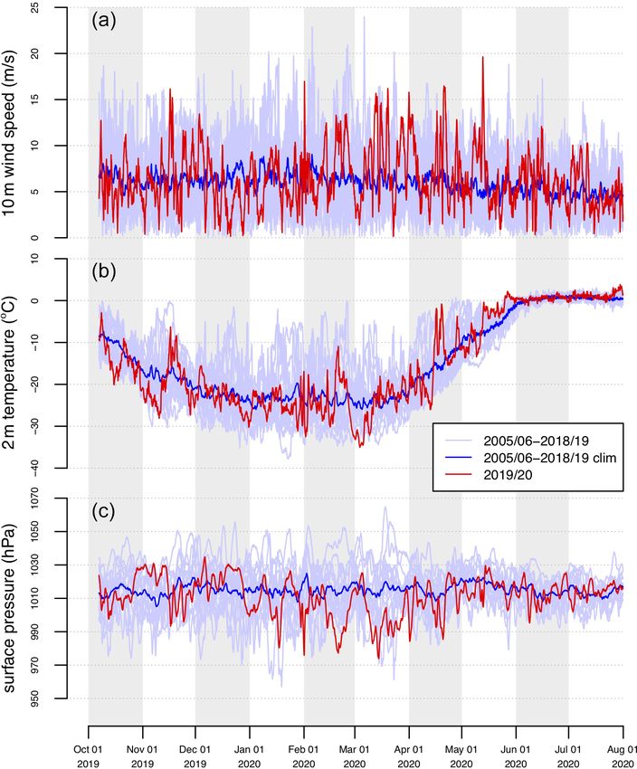
3900                                                       T. Krumpen et al.: MOSAiC drift from October 2019 to July 2020

one. The study of Krumpen et al. (2019) indicates that the          and water vapour), which can potentially mitigate some of
limited performance of IceTrack in the Fram Strait is likely        the effects, like atmospheric influence causing wrong sea ice
the result of a general underestimation of drift speeds by low-     concentrations for traditional single-parameter satellite re-
resolution satellite products in this area. It becomes particu-     trievals like the one introduced above. The spatial resolution
larly evident when looking at the reconstructed drift of the        of this data set is approximately 40 km. During and follow-
additional 23 DN buoys deployed in the vicinity of the CO           ing the warm air intrusion and the associated drizzle-on-snow
(Fig. 2c). Within the first 200 d, the reconstructed DN trajec-     event, it shows more correct ice concentrations but is yet not
tories deviate only slightly from observed tracks (28 × 15 km       available for the previous years and, thus, cannot be used as
after 200 d), but once the DN reaches the Fram Strait (south        a primary data set here.
of 82.5◦ N after 250 d), the distance between real and recon-          Based on the 89 GHz sea ice concentration data set, we
structed pathways increases exponentially. The comparison           also calculate the closest distance from the MOSAiC CO to
of the CO drift with the drift of the previous 14 years is there-   the ice edge. To remove small openings in the ice, we first
fore limited to the first 250 d.                                    smooth the sea ice concentration data set by convolution with
                                                                    a 4 × 4 (25 km) grid cell kernel; then the distances from the
2.2    Sea ice concentration                                        CO grid cell to all grid cells with zero sea ice concentration
                                                                    are calculated, and the shortest distance is selected as dis-
A time series of sea ice concentration along the MO-                tance to the ice edge.
SAiC trajectory between October to July (daily resolution)
is obtained from the 89 GHz channels of the Advanced                2.3   Sea ice thickness
Microwave Scanning Radiometer for EOS (AMSR-E) and
Advanced Microwave Scanning Radiometer 2 (AMSR2)                    Sea ice thickness (SIT) along the MOSAiC drift track dur-
on the NASA Aqua and the Japan Aerospace Exploration                ing the Arctic winter season from October 2019 through
Agency (JAXA) Global Change Observation Mission – Wa-               April 2020 is analysed using two satellite remote sensing
ter (GCOM-W) satellites, respectively (Table 1, Spreen et al.,      data sets. The first data set is based on radar altimeter data
2008; Melsheimer and Spreen, 2019a, b). Data are available          from the CryoSat-2 (CS2) mission of the European Space
from https://meereisportal.de and https://seaice.uni-bremen.        Agency (ESA). We use SIT retrievals generated at the full
de (last access: 15 February 2021). The spatial resolution of       resolution of the altimeter with an approximate point spacing
the data set is 6.25 km grid spacing (the footprint sizes of the    of 300 m and swath width of 1650 m along the ground track
two sensors are, with 4 and 5 km, even smaller). The con-           of the satellite (Table 1). The method of the SIT retrieval for
ditions in larger surroundings are determined by averaging          each radar waveform is based on Ricker et al. (2014), with
all grid points falling within a 50 and 100 km radius (com-         updates described in Hendricks and Ricker (2020). The data
pare Table 1). For comparison with previous years, we ex-           set is named the Alfred Wegener Institute (AWI) CryoSat-
tracted sea ice concentration along the MOSAiC trajectory           2 sea ice thickness product version 2.3, and it is acces-
for the years 2005–2006 to 2019–2020. The year 2011–2012            sible through the website https://meereisportal.de (last ac-
is left out due to a gap between AMSR-E and AMSR2. Un-              cess: 15 February 2021). In this study, we use the level 2
certainties (accuracy and precision) are usually below 5 %          pre-processed (L2P) product between 1 October 2019 and
for individual grid cells in winter and in the high ice con-        30 April 2020. This processing level contains data from
centration regime. In summer and at low ice concentration,          CryoSat-2 radar echoes along the ground tracks of all orbits
uncertainties can be significantly larger (up to 25 %; Spreen       within 1 d, and SIT information is provided for each radar
et al., 2008). Also, atmospheric influences like cloud liquid       footprint of approximately 300 m × 1600 m in the along- and
water and water vapour can affect the sea ice concentration         across-track direction respectively. Spatial averaging is nec-
retrieved from 89 GHz channels. However, these are uncer-           essary to reduce the significant retrieval noise for the individ-
tainties of individual grid cells and mean biases for the aver-     ual radar echoes but is not applied to the L2P data. Instead,
aged 50 and 100 km radii are lower if they are not affected         subsets of all orbit data points within 1 d are generated based
by larger-scale phenomena or summer melt. In summer or              on their distance to the noon (universal coordinated time –
during warm air intrusions, sea ice concentration underesti-        UTC) position of the CO. For each subset, we compute the
mation due to wetted ice surfaces, ice lenses or higher liq-        mean SIT, the interquartile (IQR) and interdecile (ICR) SIT
uid water content in the snow or melt ponds might occur.            range, as well as the number of data points in each daily sub-
Such a period is observed during MOSAiC from mid-April              set. According to the study logic, the search radius for the
to May 2020 and discussed below. During that time period,           SIT subsets is chosen as 50 and 100 km, and we only use in-
we show, for comparison, sea ice concentration from an in-          dividual orbits that provide at least 50 data points within the
verse multiparameter retrieval based on AMSR2 data using            specified search radii. Both the number of L2P data points
optimal estimation (Scarlat et al., 2017, 2020). It uses all fre-   per day and their minimum distance to the Polarstern noon
quency channels from 7 to 89 GHz to retrieve seven surface          position are variable. The number of CS2 L2P data points for
and atmospheric parameters (including cloud liquid water            the 50 km (100 km) search radii varies from approximately

The Cryosphere, 15, 3897–3920, 2021                                                     https://doi.org/10.5194/tc-15-3897-2021
MOSAIC DRIFT EXPEDITION FROM OCTOBER 2019 TO JULY 2020: SEA ICE CONDITIONS FROM SPACE AND COMPARISON WITH PREVIOUS YEARS - THE ...
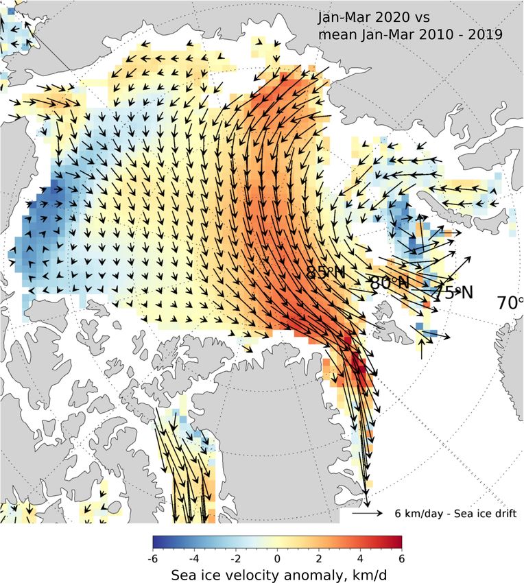
T. Krumpen et al.: MOSAiC drift from October 2019 to July 2020                                                                      3901

Figure 2. Comparison of MOSAiC CO and DN buoy tracks with IceTrack results. (a) Reproduced pathway of the CO with IceTrack. (b) Real
(GPS-based) track of the CO. (c) Distance between 23 DN buoys (source: https://seaiceportal.de, last access: 18 August 2021) deployed on
sea ice in the vicinity of the CO at the beginning of October2019 and their reconstructed trajectories. Deviation between real and virtual
tracks is small. Only once buoys enter the Fram Strait (beginning of June (day 240) at 82.5◦ N), does the distance gradually increase (red
box).

50 (300) at lower latitude to approximately 900 (2000) close           7 d, and we use the centre of this period as the reference time
to the maximum orbit coverage of CS2 at 88◦ N. No data                 to subset SIT data around the CO position at the selected
within a short period in February 2020 are found at the 50 km          radii. CS2SMOS data are based on CS2 L2P and SMOS SIT
search radius when the centre position of the search radius            data. The SMOS retrieval provides thickness information of
was above 88◦ N, while the 100 km search radius is suffi-              thin sea ice, which complements the CS2 L2P data. The data
ciently large to match CS2 orbits. We do not show data from            merging use a background field extending 2 weeks before
a smaller (e.g. 5 km) search radius, as very few orbits were           and after the observation period; thus, the temporal cover-
close enough to the CO. For the same reason we also refrain            age is shorter than that of the CS2 L2P data and ranges from
from comparing short segments of L2P data to local obser-              18 October 2019 to 12 April 2020. In addition, the selection
vations on the CO, not only because of the lower temporal              of SIT observations in the CS2SMOS data may vary from
coverage but also because the retrieval noise in the L2P SIT           the CS2 L2P regional coverage as we use the grid cell cen-
data will dominate on the scale of the local SIT observations.         tre positions within 50 and 100 km radius around the CO to
   The second data set used for the SIT estimation is the              compute the daily mean CS2SMOS SIT value. The number
merged CryoSat-2 and Soil Moisture and Ocean Salinity                  of selected CS2SMOS SIT observations depends on the po-
(SMOS; collectively CS2SMOS, version 203) SIT product                  sition of the CO relative to local grid cell coordinates. The
(Ricker et al., 2017). CS2SMOS provides gridded SIT data               number varies between 10 and 14 grid cells for the 50 km
at a resolution of 25 km, which is significantly lower than the        and between 47 and 52 for the 100 km search radius. We do
CS2 L2P data; however, the underlying optimal interpola-               not expect this variability to cause a selection bias due to the
tion provides gapless SIT information, also north of the CS2           smoothness of the CS2SMOS SIT data.
orbit limit of 88◦ N. CS2SMOS SIT estimates at the CO po-
sition during the short period when Polarstern drifted north           2.4   Snow depth
of 88◦ N are thus based on a spatial extension of SIT gra-
dients measured at the CS2 orbit limit. Each daily updated             Low-resolution snow depth along the MOSAiC trajectory is
CS2SMOS SIT field is based on an observation period of                 retrieved from the 7 and 19 GHz channels of the AMSR-E

https://doi.org/10.5194/tc-15-3897-2021                                                       The Cryosphere, 15, 3897–3920, 2021
MOSAIC DRIFT EXPEDITION FROM OCTOBER 2019 TO JULY 2020: SEA ICE CONDITIONS FROM SPACE AND COMPARISON WITH PREVIOUS YEARS - THE ...
3902                                                      T. Krumpen et al.: MOSAiC drift from October 2019 to July 2020

and AMSR2 microwave radiometer, following the method               leads and sea ice. The derived lead frequency is a temporally
from Rostosky et al. (2018). Data are available via Rostosky       integrated quantity that indicates how often a lead is found at
et al. (2019a, b). Following Rostosky et al. (2020), uncer-        a certain position within a defined period, while the lead frac-
tainties are based on Monte Carlo simulations using varying        tion is a spatially integrated quantity that provides the frac-
input parameters for a snow and sea ice (Microwave Emis-           tion of an area that was covered by leads. Note that days with
sion Model of Layered Snowpacks – MEMLS; Tonboe et al.,            a cloud fraction above 50 % are excluded from the analysis.
2006) and atmosphere (Passive and Active Microwave radia-
tive TRAnsfer – PAMTRA; Mech et al., 2020) microwave               2.6   Sea ice deformation from high-resolution radar
emission model. Most sea ice, snow and atmosphere proper-                images
ties are not known to the satellite snow depth retrieval (only
information about the ice type, multi-year or first-year is pro-   In this study, we quantify sea ice deformation based on se-
vided; based on Ye et al., 2016a, b). Thus, by varying these       quential Synthetic Aperture Radar (SAR) scenes obtained by
properties and evaluating the influence on the snow depth          ESA’s Sentinel-1A/B satellites along the drift track of the
retrieval, an estimate of the uncertainty caused by their un-      CO. Deformation is the consequence of divergence (open-
known state can be obtained. The uncertainty range for snow        ing), convergence (closing) and shear (sliding alongside)
depth on multi-year ice is between 5 to 10 cm on average (for      between ice floes. Regularly gridded sea ice drift and de-
individual grid cells it can be larger). The mean uncertainty      formation fields with a spatial resolution of 1.4 km are re-
estimate specifically for the MOSAiC data set is 8 cm. The         trieved following the method described in von Albedyll et
grid size of the snow depth data is 25 km. The snow depth re-      al. (2021). More details about the drift algorithm are pro-
trieval for multi-year ice areas is currently limited to March     vided in Thomas et al. (2008, 2011) and Hollands and Dierk-
and April, while for first-year ice it can be retrieved all win-   ing (2011). As input for the applied algorithm, we use HH-
ter (see Rostosky et al., 2018). As the MOSAiC ice floe was        polarized scenes with a spatial resolution of 50 m. Images
in an area of predominantly second-year ice, which radio-          over the CO were taken during the entire MOSAiC drift, ex-
metrically is considered multi-year ice for the snow depth re-     cept for the period between 14 January and 15 March 2020,
trieval, snow depth for MOSAiC is only available for March         when the ship was north of the satellite coverage. The tem-
and April. Here we present snow depth data for the grid cell       poral resolution is typically one image per day (with few ex-
centred at the CO (12.5 km radius) in addition to radii of 50      ceptions). Spatial derivates are calculated from the gridded
and 100 km averages (compare Table 1). A comparison with           velocity field and used to derive divergence, convergence and
previous years is made with snow depth data extracted along        shear (see von Albedyll et al., 2021 for details). To quantify
the MOSAiC drift path from 2005 until 2019.                        deformation in the vicinity of the CO, we average all grid
                                                                   cells located within a 5 km radius around the ship. Excep-
2.5    Lead detection based on optical data                        tionally strong deformation events are defined as events with
                                                                   a magnitude exceeding 2 standard deviations of the 5 km av-
Sea ice leads, i.e. lead frequencies and lead fractions            erage time series. To compare deformation in the vicinity of
along the MOSAiC drift track, are derived from Moderate-           the ship with deformation over a larger area (50 km), aver-
Resolution Imaging Spectroradiometer (MODIS) thermal in-           ages are computed for 61 5 km circles arranged within a ra-
frared data and Collection 6 (C6) of ice surface tempera-          dius of 50 km around the ship (see illustration in Fig. 3). In
tures (Hall and Riggs, 2019). In order to detect whether a         this way, we avoid biases due to scaling effects.
lead is present in a certain pixel, we employ the local surface
temperature anomaly, which is expected to exhibit signifi-         2.7   Characterization of melt pond coverage using
cant positive deviations when a lead is present during winter            optical Sentinel-2 data
(November to April). This general procedure is followed by
the application of a fuzzy inference system that assigns in-       To provide a first quantification of the spatial distribution and
dividual retrieval uncertainties to each detected lead pixel.      temporal development of large melt ponds on the MOSAiC
Using this approach, we obtain daily categorical lead maps         floe, we downloaded all available Sentinel-2 (S2, ESA) satel-
with separate classes for clouds, sea ice, leads and artefacts,    lite images (https://scihub.copernicus.eu/dhus/, last access:
with the latter comprising detected leads with an uncertainty      10 February 2021) taken over the ship between the end of
exceeding 30 %. The full approach and the resulting prod-          May and 31 July 2020. Prior to the end of May, the Sun ele-
ucts are described in Reiser et al. (2020). From this data set,    vation was not high enough for passive optical remote sens-
we use daily lead data with a spatial resolution of 1 km for       ing. A total of eight completely or partially cloud-free scenes
the months of November to April for the years of 2005–2006         could be identified. For the detection of melt ponds, we se-
to 2018–2019 (as the reference period) and for the winter of       lected five scenes that are temporally equally spaced, namely
2019–2020 (for MOSAiC, compare Table 1). The daily lead            21 June, 1 July, 7 July, 22 July and 27 July 2020. Next, the
data can only be derived for winter months as the retrieval        MOSAiC floe was clipped, and a pond index was calculated
relies on a significant surface temperature contrast between       by means of a normalized spectral index (e.g. Gignac et al.,

The Cryosphere, 15, 3897–3920, 2021                                                    https://doi.org/10.5194/tc-15-3897-2021
MOSAIC DRIFT EXPEDITION FROM OCTOBER 2019 TO JULY 2020: SEA ICE CONDITIONS FROM SPACE AND COMPARISON WITH PREVIOUS YEARS - THE ...
T. Krumpen et al.: MOSAiC drift from October 2019 to July 2020                                                                     3903

Figure 3. To compare deformation in the vicinity of the ship (5 km) with deformation on larger scales (50 km), averages were computed for
61 5 km circles arranged within a radius of 50 km around the ship. Example of divergence, convergence (a) and shear (b) derived from two
consecutive Sentinel-1 SAR images acquired on 14 April (07:26:14 UTC) and 15 (08:07:03 UTC) 2020. Sea ice motion is displayed as black
arrows. The image pair shows the strongest deformation event observed. Within 24 h, a 2.5 km wide north–south-oriented lead opened up
∼ 25 km away from the CO.

2017; Watson et al., 2018) using S2 bands 4 (665 nm) and 8             3     Results and discussion
(842 nm) as input. The pond index is used to differentiate be-
tween water and ice/snow. Note that only ponds larger than             3.1    Atmospheric conditions and the Transpolar Drift
the spatial resolution of the S2 sensor (10 m) can be detected.               in 2019–2020
We, therefore, assume that the actual pond cover is signifi-
cantly underestimated, and that the method is only suitable
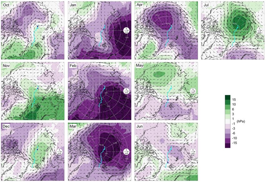
for providing estimates of the timing and relative changes in          Large-scale surface air pressure and associated anomalies in
pond coverage.                                                         10 m wind speed (shown in Fig. 4) determined the course
                                                                       of the MOSAiC drift and its deviation from the long-term
2.8   Reanalysis and ship weather data                                 average. October, November and December were character-
                                                                       ized by moderate monthly mean circulation anomalies, ori-
Mean sea level pressure, 2 m air temperature and 10 m                  ented mostly such that the winds (and thus the drift) were
wind speed data for the time period 2005–2020 are                      westward rather than northward, thereby preventing the MO-
taken from the newest version of the European Centre                   SAiC floe from reaching the North Pole (note that Fig. 4
for Medium-Range Weather Forecasts (ECMWF) global                      shows wind anomalies, whereas the drift path is the actual
reanalysis, ERA5 (Hersbach et al., 2020). Hourly val-                  drift). Starting in January, large-scale low pressure entered
ues along the MOSAiC trajectory in 2019–2020 and                       the Arctic from the European sector, resulting in an inten-
in the preceding 14 years along the same trajectory                    sification of the Transpolar Drift in January, February and
are extracted by linear interpolation in time and space                March (Fig. 5), with the low-pressure region gradually mov-
after triangulation of the rectangular 0.25◦ ERA5 grid.                ing towards the Beaufort Sea. Correspondingly, these months
The 2019–2020 trajectory data are evaluated against                    were associated with an exceptionally high positive Arctic
corresponding standard meteorological observations on                  Oscillation (AO) index (see Dethloff et al., 2021, and Rinke
board the Polarstern (https://www.awi.de/nc/en/science/                et al., 2021, for a more detailed description). In April, the
long-term-observations/atmosphere/polarstern.html, last ac-            decaying low-pressure centre was located over the Beaufort
cess: 22 February 2021). The ship measurements are, how-               Sea, resulting in a drift of the MOSAiC floe towards the Bar-
ever, taken at non-standard heights (wind – 39 m; air tem-             ents Sea. Next, the reversed air pressure gradient in May,
perature – 29 m; pressure – 16 m, reduced to sea level) so             with a high-pressure anomaly over the Beaufort Sea, pushed
the evaluation is rather qualitative. More stringent compar-           the MOSAiC floe towards northeastern Greenland until it en-
isons of MOSAiC in situ meteorological observations, not               tered the Fram Strait area (June–July).
just from the ship but from a large number of sensors across              Figure 6 compares ERA5-based atmospheric conditions
the CO and DN, are beyond the scope of this paper but will             along the MOSAiC drift trajectory with conditions in the
be conducted elsewhere.                                                preceding 14 years. The circulation anomalies from January
                                                                       through May (Fig. 4) led to positive air temperature anoma-
                                                                       lies in northern Siberia and in the Kara and Laptev seas, in
                                                                       particular in February (up to +10 K; not shown). In con-

https://doi.org/10.5194/tc-15-3897-2021                                                      The Cryosphere, 15, 3897–3920, 2021
MOSAIC DRIFT EXPEDITION FROM OCTOBER 2019 TO JULY 2020: SEA ICE CONDITIONS FROM SPACE AND COMPARISON WITH PREVIOUS YEARS - THE ...
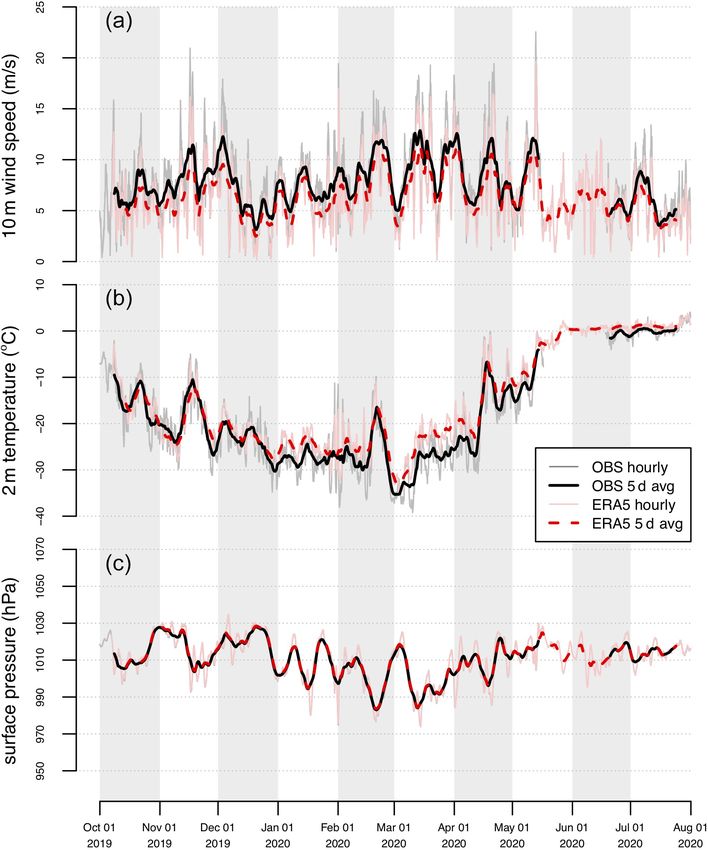
3904                                                         T. Krumpen et al.: MOSAiC drift from October 2019 to July 2020

Figure 4. Monthly mean sea level air pressure (shading) and 10 m wind (arrows) anomalies with respect to the reference period of 2005–2019
for each month of the MOSAiC drift from October 2019 to July 2020. The complete drift path is denoted by cyan lines; the drift during the
respective month is denoted by blue arrows.

trast, air temperature anomalies at the MOSAiC floe were               sessments (e.g. Batrak and Müller, 2019). Note that the true
rather moderate most of the time (Fig. 6; middle). Moder-              2 m air temperature bias might be even larger because the
ate warmer-than-average periods occurred in mid-November,              ship air temperatures might be overestimated due to (i) lo-
late February, mid-April and late May, whereas colder-                 cal heat sources and (ii) higher temperatures at the measure-
than-average periods occurred in early November and early              ment height of 29 m compared to 2 m in typical cases of near-
March, with absolute minima around −35 ◦ C. Wintertime                 surface inversion. Given that these differences are likely sys-
cold (warm) anomalies were typically associated with high              tematic and, thus, similar in other years, the anomalies dis-
(low) surface air pressure anomalies (Fig. 6; bottom). The             cussed above are likely not strongly affected.
positive AO months of January, February, March and April
were accompanied by low-pressure anomalies at the MO-                  3.2   The MOSAiC drift and a comparison to previous
SAiC floe (Fig. 6 bottom). High wind speeds were encoun-                     years
tered in particular in these months but also in late November
and early December (Fig. 6 top). Apart from these excep-
                                                                       We compared the drift of the MOSAiC floe with the course
tions, meteorological conditions at the MOSAiC floe can be
                                                                       the CO would have taken if the experiment had started in
considered average compared to previous years.
                                                                       any of the previous 14 years (October 2005–2018). The un-
   The ERA5 data along the MOSAiC trajectory in 2019–
                                                                       derlying satellite-based Lagrangian tracking approach is in-
2020 agree well with co-located ship observations (Fig. 7),
                                                                       troduced in Sect. 2.1. Figure 8 summarizes the results of
in particular regarding surface air pressure. Wind speed tends
                                                                       this analysis. Figure 8a shows the reproduced MOSAiC tra-
to be slightly lower in ERA5, although it should be noted
                                                                       jectory (multicoloured line) together with trajectories from
that the comparison with the raw on-board observations (e.g.
                                                                       previous years (gray lines). The large differences between
winds are measured at 39 m instead of 10 m) has limitations.
                                                                       the tracks show how difficult it is to accurately predict the
However, the winter warm bias in ERA5 over Arctic sea ice
                                                                       course of a drifting platform and how large the spread of
of the order of 2–3 K (Fig. 7) is consistent with previous as-
                                                                       possible endpoints can be. Figure 8b provides the averaged

The Cryosphere, 15, 3897–3920, 2021                                                         https://doi.org/10.5194/tc-15-3897-2021
MOSAIC DRIFT EXPEDITION FROM OCTOBER 2019 TO JULY 2020: SEA ICE CONDITIONS FROM SPACE AND COMPARISON WITH PREVIOUS YEARS - THE ...
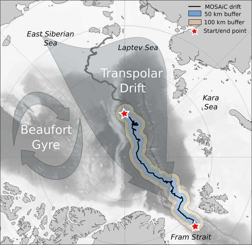
T. Krumpen et al.: MOSAiC drift from October 2019 to July 2020                                                                   3905

                                                                       black line – i.e. containing the underestimation in April dis-
                                                                       cussed below; Spreen et al., 2008). The seasonal evolution
                                                                       is characterized by a substantial temporal variability over the
                                                                       course of the 303 d long drift. This variability is almost inde-
                                                                       pendent of the spatial scale used with only minor differences
                                                                       (±0.5 % deviation from mean) between the sea ice concen-
                                                                       tration values determined from the 3, 50 and 100 km radius
                                                                       (Fig. 10).
                                                                          Given the high agreement between the values from differ-
                                                                       ent radii, we focus, in the following discussion, on the time
                                                                       series with the highest resolution (3 km radius; Fig. 9). The
                                                                       October to July sea ice concentration average along the MO-
                                                                       SAiC drift trajectory agrees well with the long-term 2005–
                                                                       2006 to 2019–2020 average (both have a mean of 97 %).
                                                                       However, on shorter timescales there are significant differ-
                                                                       ences. During the first half of the drift (October until end of
                                                                       February) the MOSAiC ice concentration was, with 99.5 %,
                                                                       about 1 % higher than the long-term average (compare black
                                                                       line with blue; Fig. 9), while during the second half (March
                                                                       until end of July), it was lower than during the long-term av-
                                                                       erage and showed higher variability than the first half. High
                                                                       ice concentration, like 99.5 %, is not unusual (compare to the
                                                                       gray lines) and can be expected in winter in the central Arc-
Figure 5. The 3-month (January–March) sea ice velocity anomalies
                                                                       tic (e.g. Kwok, 2002). The second half with lower (actually
in 2020 with respect to the reference period 2010–2019. Anoma-         false) ice concentration is more unusual and will be discussed
lies were computed from the OSI-405-c motion product provided          further in the following.
by the Ocean and Sea Ice Satellite Application Facility (OSI SAF;         Sea ice concentration variability stayed below 5 % until
Lavergne, 2016). The vectors plotted on top indicate the average       March 2020, when first significant reductions in ice concen-
daily sea ice motion for the same period (reprinted from Dethloff et   tration occurred. At this time, the CO was already positioned
al., 2021).                                                            north of the Fram Strait, and the distance to the ice edge
                                                                       was gradually decreasing (compare Fig. 11). With the on-
                                                                       set of spring in March–April, the first major drops in ice
satellite-derived daily displacement rates of the MOSAiC CO            concentration below 90 % occurred. The strong ice concen-
during the first 250 d as compared to the previous 14 years.           tration reductions down to 75 % from mid-April until mid-
With 8.52 km/d, the drift speed in 2019–2020 is around 20 %            May (average ice concentration of 87 %) were due to a false
higher than the mean over the period from 2005 to 2018                 satellite ice concentration retrieval. Visual observations from
(7.14 km/d × 0.75). Only 2008–2009 shows an even higher                the ship’s bridge confirm that the ice concentration, on av-
average displacement rate (8.79 km/d), although the Fram               erage, stayed higher than 95 % during that time period. We
Strait is reached a few days later due to a more northerly             can see that, at that time, a warm air intrusion raised tem-
route. Another striking year is 2018–2019, with only av-               peratures close to 0 ◦ C, which was accompanied by a signif-
erage daily displacement rates but a strong westward drift             icant increase in wind speed (Fig. 6). The warming induced
component, which would have carried the ship even faster               strong temperature gradients and increased vapour fluxes in
toward Fram Strait than in 2019–2020. A trend towards a                the snow, which can cause stronger snow metamorphism and
faster Transpolar Drift, as reported by Spreen et al. (2011)           significantly change the snow permittivity already at above
or Krumpen et al. (2019), cannot be deduced from this rather           −5 ◦ C snow temperatures (Mätzler, 1987). Also, liquid wa-
simple and spatially limited analysis. However, results shown          ter content can increase at temperatures slightly below 0 ◦ C,
here are in line with these studies.                                   and small liquid water fractions of, e.g., 2 % strongly change
                                                                       the microwave loss in the snow (Hallikainen, 1986). Refreez-
3.3   Sea ice concentration                                            ing after the warming event can cause ice lenses in the snow.
                                                                       Such events were previously observed to have an influence
Sea ice concentration along the MOSAiC drift trajectory in             on microwave properties and penetration (e.g. King et al.,
2019–2020 and the reference period (2005–2006 to 2018–                 2018). On April 2019, slight drizzle was observed, which
2019) is shown in Fig. 9. The average sea ice concentration            likely refroze on the snow afterwards. These surface pro-
between 4 October 2019 and 31 July 2020 amounts to 97 %                cesses and additional weather influence by high water vapour
(based on the 89 GHz sea ice concentration – shown with the            and cloud liquid water affect the microwave polarization dif-

https://doi.org/10.5194/tc-15-3897-2021                                                     The Cryosphere, 15, 3897–3920, 2021
MOSAIC DRIFT EXPEDITION FROM OCTOBER 2019 TO JULY 2020: SEA ICE CONDITIONS FROM SPACE AND COMPARISON WITH PREVIOUS YEARS - THE ...
3906                                                       T. Krumpen et al.: MOSAiC drift from October 2019 to July 2020

Figure 6. Hourly atmospheric conditions along the MOSAiC drift trajectory according to ERA5 in 2019–2020 (red) and in the preceding
14 years (light blue; average in dark blue). Panels show the (a) 10 m wind speed, (b) 2 m air temperature and (c) surface air pressure,
respectively. See Fig. 7 for a comparison with corresponding ship observations.

ference (e.g. Lu et al., 2018) and likely caused the strong           like in our 2020 case. After mid-May 2020, the ice concen-
fluctuation in ice concentration for the ASI algorithm used           tration recovered to almost 100 %. In July, the floe started to
here. Other ice concentration algorithms for AMSR2 satellite          disintegrate and ice concentration dropped to 85 % within a
data (e.g. NASA team) showed similar effects (not shown).             radius of 3 km around Polarstern, and below 60 % in the 50
As an alternative, we present the ice concentration from an           and 100 km radii (Fig. 10).
optimal estimation retrieval (Scarlat et al., 2018, 2020) dur-           We determine the closest distance to the ice edge from
ing that critical time period in Fig. 9, which attempts to take       sea ice concentration maps (Fig. 11). At the beginning of
such effects into account (specifically the atmospheric in-           the MOSAiC expedition, the distance from the CO to the ice
fluence), and in our case, it is in better agreement with the         edge was about 320 km. During October, the distance gradu-
ship-based observations. Also, in previous years (gray lines;         ally increased to 1000 km due to the freeze-up of the Russian
Fig. 9) occasionally ice concentrations below 90 % were ob-           marginal seas. Once the MOSAiC CO approached the Fram
served in the sea ice concentration record during mid-winter.         Strait (March 2020), the distance to the ice edge steadily de-
We have not investigated if these were real openings in the           creased until the ice margin was reached at the end of July
ice caused by ice divergence or atmosphere-induced effects

The Cryosphere, 15, 3897–3920, 2021                                                       https://doi.org/10.5194/tc-15-3897-2021
T. Krumpen et al.: MOSAiC drift from October 2019 to July 2020                                                                        3907

Figure 7. Atmospheric conditions along the MOSAiC drift trajectory in 2019–2020 according to ERA5 (red and light red) and according to
ship measurements (black and gray). Hourly data are depicted in light red and gray; the 5 d averages are depicted in red (dashed) and black.
Panels show the (a) 10 m wind speed, (b) 2 m air temperature and (c) surface air pressure, respectively.

2020. Note that the winter variability in ice edge distance             3.4    Sea ice thickness
was caused by polynya activity in the Russian shelf seas.
   Future studies will investigate the impact of the warm air           Both satellite-based sea ice thickness products show the ex-
intrusion on microwave properties in more detail based on               pected increase in ice thickness between October 2019 and
the extensive in situ microwave and snow/ice measurements               April 2020 (Fig. 12 and Table 2). Except for the period be-
conducted on the MOSAiC floe. However, the smaller fluctu-              tween 14 February to 8 March 2020, when the CO was po-
ations of the sea ice concentration between 97 % and 100 %              sitioned north of 88◦ N, the high orbit density of CS2 allows
during October to February need further investigation by                almost continuous daily coverage at 50 and 100 km radius.
combining them more closely with the different lead fraction            The monthly mean thickness within a 50 km (100 km) radius
and ice divergence records discussed below. This will help us           around the CO changed from 0.77 m (0.8 m) in October 2019
to investigate the partitioning between thermodynamic and               to 2.40 m (2.51 m) in April 2020. The sea ice thickness distri-
dynamic redistribution of ice mass, as well as the impact of            bution is characterized by the IQR (difference between 75 %
ocean to atmosphere heat fluxes.                                        and 25 % percentile) and the interdecile range (IDR; differ-
                                                                        ence between 90 % and 10 % percentile; compare Sect. 2.
                                                                        The increase in sea ice thickness was accompanied by a simi-

https://doi.org/10.5194/tc-15-3897-2021                                                        The Cryosphere, 15, 3897–3920, 2021
3908                                                           T. Krumpen et al.: MOSAiC drift from October 2019 to July 2020

                                                                        larger differences in sea ice thickness of 36 % between the
                                                                        DN area and areas further away.
                                                                           Results from CS2SMOS mirror these findings of thinner
                                                                        ice close to the CO compared to the larger scale, though dif-
                                                                        ferences are smaller (Fig. 12; Table 2). This can be expected,
                                                                        as the primary input to the CS2SMOS analysis in the central
                                                                        Arctic is CS2 data due to its higher sensitivity to thicker ice
                                                                        than SMOS. The main differences to CS2 L2P are therefore
                                                                        the influence of SMOS in the beginning of the winter and the
                                                                        larger degree of smoothing introduced by the optimal inter-
                                                                        polation. The monthly mean sea ice thickness values in Ta-
                                                                        ble 2 are therefore mainly consistent, with the exception of
                                                                        October and November 2019. In this period, CS2SMOS was
                                                                        consistently higher by approximately 0.15 m with respect to
                                                                        the CS2 L2P data.
                                                                           We do not expect that the locally lower thicknesses in the
                                                                        DN are well represented in the CS2SMOS SIT, since these
                                                                        are influenced by a larger region due to the interpolation
Figure 8. A comparison of the MOSAiC drift with the drift of pre-
                                                                        method. The CS2 L2P thicknesses instead are effectively
vious years. (a) Results from a forward-tracking experiment. Sea        point measurements at kilometre scale and are apparently
ice was traced 14 times in a forward direction for a period of 250 d,   able to pick up the local thickness gradient with thickness
starting on 4 October (2005–2019) from the position where the Po-       differences smaller than the uncertainty of absolute SIT val-
larstern drift started (red star). The multicoloured trajectory line,   ues. The discrepancy between the CS2 L2P and CS2SMOS
with colours corresponding to the month of year, indicates the re-      thicknesses persisted well into November 2019 and became
produced drift of the MOSAiC CO (Central Observatory). All other        less prominent afterwards. This provides evidence that the
years (2005–2018) are shown as black lines. The end nodes of the        local thickness minimum at the MOSAiC DN became less
individual tracks are marked by a black circle. (b) Averaged dis-       prominent over the winter season, though still at a detectable
placement of sea ice per day (kilometres) for individual years.         level as indicated by the consistent but minor differences at
                                                                        radii of 50 and 100 km.
                                                                           Since CS2 L2P and CS2SMOS are in general consistent
larly increased IQR and IDR, indicating a wider sea ice thick-          over the winter season, we use CS2SMOS data to compare
ness distribution as a result of thermodynamic ice growth and           sea ice conditions during the MOSAiC drift with the past
deformation of the older ice class and the formation of young           nine winter seasons in the CS2SMOS data record (Fig. 13).
ice throughout the winter season. Specific dynamic events               The comparison between the years shows a comparably low
sensed by other remote sensing sensors have a visible im-               sea ice thickness in the 10-year-long data record at the lo-
pact on the change of mean SIT and, thus, the apparent SIT              cation of the MOSAiC expedition, if not the lowest for seg-
growth rates. Lead formation in mid-November 2019, also                 ments in the earlier part of the drift. The monthly sea ice
seen in a strong divergence event, added new thin ice coin-             thickness during MOSAiC was approximately 0.4 m lower
cides with an intermittent SIT decrease (Fig. 19). The SIT              at the beginning of the drift compared to mean monthly
distribution in the second half of April 2020 also widened              CS2SMOS of all previous winters (Table 2). The differences
significantly at a time when both lead fractions and a drop in          reduced towards 0.3 m in April, indicating slightly stronger
sea ice concentration indicates the presence of new ice for-            thermodynamic and dynamic ice growth with respect to the
mation.                                                                 average, potentially aided by the thinner sea ice at the begin-
   It is also notable that the CS2 L2P sea ice thickness was, on        ning. These results are, however, based on a SIT data record
average, consistently thinner at the 50 km radius compared              that depends on climatological values for snow load and sea
to the 100 km radius (Table 2; on average 6 cm (4 %) thinner            ice density and, thus, does not contain the impact by the ex-
between October and April). Similarly, IQR and IDR were                 pected variability in these parameters in the SIT retrieval. For
larger for 100 km than for 50 km; however, the larger num-              example, using dynamic snow load in SIT retrieval by satel-
ber of data points in the wider search area may also lead to            lite radar altimeter has resulted in a more pronounced inter-
a higher likelihood of diverse sea ice conditions. This is in           annual variability but also stronger thickness trends in the
agreement with findings of Krumpen et al. (2020). Accord-               Arctic marginal seas (Mallett et al., 2021). While MOSAiC
ing to the authors, the MOSAiC DN was set up at a regional              has taken place in the central Arctic with generally thicker
thickness minimum. The local minimum is related to the ice              ice and snow, a similar impact can be expected as well. We
age. Sea ice in the DN was formed 3 weeks later than the sur-           therefore consider it unlikely that the differences between the
rounding ice. However, Krumpen et al. (2020) report even                SIT estimates along the MOSAiC drift tracks for the 10 years

The Cryosphere, 15, 3897–3920, 2021                                                        https://doi.org/10.5194/tc-15-3897-2021
T. Krumpen et al.: MOSAiC drift from October 2019 to July 2020                                                                        3909

Figure 9. Sea ice concentration within a 3 km radius around the CO (6.25 km grid cell; black) along the MOSAiC drift from 4 October 2019
to 31 July 2020 in comparison to the ice concentrations from 2005–2006 to 2018–2019 for the same drift trajectory. The blue line shows the
average for 2005–2006 to 2018–2019, while the gray lines show the individual years. All time series are smoothed with a 5 d running mean.
During spring, warm air intrusions caused a significant temporary reduction in the sea ice concentration (dashed black line). We, therefore,
show that with uncertainty estimates, in addition to an alternative sea ice concentration data set during the time (red and shaded red; not
available for the climatology; see main text).

Figure 10. Sea ice concentration along the MOSAiC drift trajectory from the start of the drift on 4 October 2019 until the end of the first
floe on 31 July 2020. Daily (no smoothing) sea ice concentrations are shown at 3.125 (black), 50 (blue) and 100 km (yellow) radii. Note the
significantly underestimated concentrations between mid-April to May and the associated discussion in the main text and Fig. 9.

                                                                        of CS2SMOS data can be explained by retrieval uncertainty
                                                                        alone. Field observations with longer time series are needed
                                                                        to evaluate the stability of SIT retrievals over decadal periods
                                                                        (e.g. Khvorostovsky et al., 2020), which are not available for
                                                                        the location of MOSAiC.
                                                                           CS2SMOS also indicates sea ice thickness differences be-
                                                                        tween the 50 km radius and the 100 km radius, showing that
                                                                        the MOSAiC expedition took place in a local sea ice thick-
                                                                        ness minimum. It should be noted that the SIT differences,
                                                                        specifically between the two search radii, were well below
                                                                        the uncertainty estimate of the retrieval for both CS2SMOS
                                                                        and CS2. Gridded CS2 data indicate a retrieval uncertainty,
Figure 11. Distance of the MOSAiC CO to the ice edge obtained
                                                                        on average of 0.5 and 0.7 m, between October 2019 and
from the sea ice concentration data set.
                                                                        April 2020 at a scale of 25 km and monthly periods (Hen-
                                                                        dricks and Ricker, 2020). The main driver of the uncertainty

https://doi.org/10.5194/tc-15-3897-2021                                                        The Cryosphere, 15, 3897–3920, 2021
3910                                                           T. Krumpen et al.: MOSAiC drift from October 2019 to July 2020

Figure 12. Daily sea ice thickness estimates from CryoSat-2 (CS2) full-resolution orbit L2P data and gridded CryoSat-2/SMOS (CS2SMOS)
multi-sensor thickness analysis extracted for two different search radii (50 and 100 km) centred around the noon position of the CO for each
day of the drift. Results from L2P data are only present for days where at least 50 L2P data points are found in both search radii. The gray
rectangle indicates when the CO drifted north of 88◦ N and outside the CS2 orbit coverage. The distribution of CS2 orbit data within the
search radii is described by the mean value, interquartile (25 % to 75 % percentiles) and interdecile ranges (10 % to 90 % percentiles). For
CS2SMOS, only the mean values of grid values within the search radius are provided.

Table 2. Monthly statistics of sea ice thickness (SIT) from CryoSat-2 (CS2) level 2P (L2P) orbit and gridded CryoSat-2/SMOS (CS2SMOS)
data for two radii around the CO position. The CS2 SIT distribution is characterized by the interquartile range (IQR) as the difference between
the 75 % and 25 % percentile and the interdecile range (IDR) as the difference between the 90 % and 10 % percentile. For CS2SMOS, the
SIT difference (1SIT) between the MOSAiC year and SIT from the same drift trajectory, but of previous winters since 2010, is given. The
asterisk (∗ ) indicates that the mean SIT of CS2SMOS depends on fewer years than the other month since the CS2SMOS data record only
starts in November 2010.

                                                     CS2 L2P                                             CS2SMOS
                                SIT (m)            SIT IQR (m)         SIT IDR (m)             SIT (m)            1SIT (m)
                            50 km     100 km     50 km    100 km     50 km     100 km     50 km     100 km      50 km    100 km
              Oct 2019∗       0.77        0.80    0.47       0.51      0.93       1.04      0.95         0.97   −0.41     −0.38
              Nov 2019        1.02        1.07    0.52       0.60      1.05       1.23      1.13         1.15   −0.45     −0.43
              Dec 2019        1.26        1.31    0.57       0.62      1.14       1.27      1.35         1.37   −0.38     −0.35
              Jan 2020        1.46        1.48    0.61       0.63      1.21       1.28      1.50         1.51   −0.38     −0.36
              Feb 2020        1.90        1.99    0.69       0.79      1.39       1.60      1.99         2.00   −0.29     −0.28
              Mar 2020        2.23        2.27    0.85       0.88      1.74       1.81      2.31         2.33   −0.43     −0.41
              Apr 2020        2.40        2.51    1.21       1.24      2.33       2.40      2.50         2.51   −0.29     −0.27

magnitude, however, is less retrieval noise but rather the un-            though the absolute SIT uncertainty remains substantial. The
certainty of auxiliary parameters such as snow load and sea               finding of consistently thinner ice for the 50 km search ra-
ice density. The deviation between actual values of these pa-             dius compared to the 100 km search radius throughout the
rameters and their parameterizations in the satellite retrieval           drift might be seen as a demonstration of this point.
is likely to have larger correlation length scales. Thus, the                Future work with the MOSAiC field data will focus on im-
satellite sensors might be able to sense local SIT differences,           proving accuracy of SIT retrievals as well as quantifying its

The Cryosphere, 15, 3897–3920, 2021                                                            https://doi.org/10.5194/tc-15-3897-2021
T. Krumpen et al.: MOSAiC drift from October 2019 to July 2020                                                                   3911

                                                                       than the detected snowfall by several sensors in the MOSAiC
                                                                       CO (about 10–20 mm snow water equivalent, i.e. approx. 4–
                                                                       8 cm snow depth; Wagner et al., 2021). However, the Wag-
                                                                       ner et al. (2021) study also shows that snowfall does not al-
                                                                       ways directly relate to snow depth increases because lateral
                                                                       snow redistribution plays a significant role. Future studies
                                                                       will evaluate the satellite snow depth in more detail based
                                                                       on the extensive snow measurements taken during MOSAiC.
                                                                          The satellite AMSR-E/2 March–April 2020 snow depth
                                                                       of 22 cm is significantly lower than the snow climatology
                                                                       from Warren et al. (1999) for the years 1954 to 1991. For
                                                                       that depth, the March–April snow depth for the MOSAiC re-
                                                                       gion would have been between 35 and 39 cm, i.e. 60 % to
                                                                       80 % higher than during MOSAiC and the whole AMSR-E/2
                                                                       time period from 2005 to 2019 (green line in Fig. 14). Thus,
                                                                       we observe a strong reduction in snow depth for the MO-
                                                                       SAiC region compared to previous decades. This also has
                                                                       implications for ice thickness retrievals from satellite altime-
                                                                       ters, where the Warren snow depth climatology often is used
                                                                       for the freeboard to ice thickness conversion (Sect. 2.3; e.g.
Figure 13. Daily sea ice thickness from gridded CryoSat-2/SMOS         Ricker et al., 2014).
(CS2SMOS) multi-sensor thickness analysis extracted within 50 km          Here we only present one satellite-based snow depth
of the CO noon position for all Arctic winters in the CS2SMOS data     product. Future studies will compare our snow depth re-
record. Each winter season is marked by the start and end year, e.g.   trievals from the AMSR-E/2 microwave radiometers with
2011–2012. The bold black line indicates data during the MOSAiC        snow depth from combined CryoSat-2 and ICESat-2 mea-
year and is identical to the 50 km radius CS2SMOS data in Fig. 12.     surements (Kwok et al., 2020) and snow depth from SMOS
                                                                       (Maaß et al., 2013).

true magnitude. But given the sensitivity of present-day SIT           3.6   Leads
products to local thickness differences and their sensitivity
to dynamic events captured by other sensors, the question re-          The mean winter lead frequency (November to April be-
mains how SIT data at high spatial and temporal resolution             tween 2005–2006 and 2018–2019) for the central Arctic
can be used to better observe and understand the dynamics              Basin and adjacent seas is shown in Fig. 15a. The climatol-
of the sea ice cover.                                                  ogy shows that between November and April the central Arc-
                                                                       tic Ocean is generally characterized by low lead frequencies
3.5   Snow depth                                                       with values of roughly 0.1. This agrees well with consistently
                                                                       high ice concentration values indicated by the sea ice con-
Figure 14 shows a time series of satellite-based snow thick-           centration climatology during the first half of the expedition
ness in March–April for the years between 2005 and 2020.               (Fig. 9). According to the climatology, higher lead frequen-
The mean March–April snow depth during the MOSAiC year                 cies (> 0.15) in winter are only to be expected near the ice
was 22 cm at the 12.5 km radius (22 or 23 cm in 50 or 100 km           edge and in the Fram Strait. The lead frequency anomalies
radius) with an uncertainty of 5 cm. Note that the observed            for the MOSAiC year 2019–2020 shown in Fig. 15b indicate
snow thickness during MOSAiC is around 3 cm lower than                 no significant deviations from the winter mean climatology.
the long-term average of the period 2005 to 2019. A prelim-            On average, anomalies were slightly negative along the MO-
inary comparison (not shown) of satellite-based snow thick-            SAiC drift trajectory and in the sector between 30◦ W and
ness estimates with in situ observations from the MOSAiC               120◦ E, which again agrees well with the observed slightly
CO indicates a good agreement with errors not exceeding the            higher ice concentration values as compared to the long-term
expected uncertainty of on average 5 cm.                               mean (Fig. 9).
   The snow depth during MOSAiC was a few centimetres                     Regional differences in lead frequencies can be inferred
lower but, overall, quite average compared to the long-term            from monthly lead anomaly maps shown in Fig. 15c–h.
mean. The time series in Fig. 14 shows that the snow depth             The monthly maps reveal anomalously high lead frequencies
stayed almost constant from beginning of March until mid-              north of Greenland and Ellesmere Island between Novem-
April. Only after the warm air intrusion in April (Fig. 6), did        ber 2019 and January 2020. Moreover, the strong positive
increased precipitation lead to a small increase in snow depth         anomalies in the Barents Sea in January 2020 and in the
of about 3 cm. This is in agreement but potentially a bit lower        Beaufort Sea in February–March 2020 are worth mentioning

https://doi.org/10.5194/tc-15-3897-2021                                                     The Cryosphere, 15, 3897–3920, 2021
You can also read