Climate change in the High Mountain Asia in CMIP6 - Earth ...
←
→
Page content transcription
If your browser does not render page correctly, please read the page content below
Research article
Earth Syst. Dynam., 12, 1061–1098, 2021
https://doi.org/10.5194/esd-12-1061-2021
© Author(s) 2021. This work is distributed under
the Creative Commons Attribution 4.0 License.

            Climate change in the High Mountain Asia in CMIP6
          Mickaël Lalande1 , Martin Ménégoz1 , Gerhard Krinner1 , Kathrin Naegeli2 , and Stefan Wunderle2
                            1 Univ.Grenoble Alpes, CNRS, IRD, G-INP, IGE, 38000 Grenoble, France
              2 Institute   of Geography and Oeschger Center for Climate Change Research, University of Bern,
                                                    3012 Bern, Switzerland
                       Correspondence: Mickaël Lalande (mickael.lalande@univ-grenoble-alpes.fr)

                                       Received: 16 June 2021 – Discussion started: 24 June 2021
                                       Accepted: 23 August 2021 – Published: 2 November 2021

      Abstract. Climate change over High Mountain Asia (HMA, including the Tibetan Plateau) is investigated over
      the period 1979–2014 and in future projections following the four Shared Socioeconomic Pathways: SSP1-2.6,
      SSP2-4.5, SSP3-7.0 and SSP5-8.5. The skill of 26 Coupled Model Intercomparison Project phase 6 (CMIP6)
      models is estimated for near-surface air temperature, snow cover extent and total precipitation, and 10 of them
      are used to describe their projections until 2100. Similarly to previous CMIP models, this new generation of
      general circulation models (GCMs) shows a mean cold bias over this area reaching −1.9 [−8.2 to 2.9] ◦ C (90 %
      confidence interval) in comparison with the Climate Research Unit (CRU) observational dataset, associated
      with a snow cover mean overestimation of 12 % [−13 % to 43 %], corresponding to a relative bias of 52 %
      [−53 % to 183 %] in comparison with the NOAA Climate Data Record (CDR) satellite dataset. The temperature
      and snow cover model biases are more pronounced in winter. Simulated precipitation rates are overestimated
      by 1.5 [0.3 to 2.9] mm d−1 , corresponding to a relative bias of 143 % [31 % to 281 %], but this might be an
      apparent bias caused by the undercatch of solid precipitation in the APHRODITE (Asian Precipitation-Highly-
      Resolved Observational Data Integration Towards Evaluation of Water Resources) observational reference. For
      most models, the cold surface bias is associated with an overestimation of snow cover extent, but this relationship
      does not hold for all models, suggesting that the processes of the origin of the biases can differ from one model
      to another. A significant correlation between snow cover bias and surface elevation is found, and to a lesser
      extent between temperature bias and surface elevation, highlighting the model weaknesses at high elevation. The
      models with the best performance for temperature are not necessarily the most skillful for the other variables,
      and there is no clear relationship between model resolution and model skill. This highlights the need for a better
      understanding of the physical processes driving the climate in this complex topographic area, as well as for
      further parameterization developments adapted to such areas. A dependency of the simulated past trends on the
      model biases is found for some variables and seasons; however, some highly biased models fall within the range
      of observed trends, suggesting that model bias is not a robust criterion to discard models in trend analysis. The
      HMA median warming simulated over 2081–2100 with respect to 1995–2014 ranges from 1.9 [1.2 to 2.7] ◦ C
      for SSP1-2.6 to 6.5 [4.9 to 9.0] ◦ C for SSP5-8.5. This general warming is associated with a relative median
      snow cover extent decrease from −9.4 % [−16.4 % to −5.0 %] to −32.2 % [−49.1 % to −25.0 %] and a relative
      median precipitation increase from 8.5 % [4.8 % to 18.2 %] to 24.9 % [14.4 % to 48.1 %] by the end of the century
      in these respective scenarios. The warming is 11 % higher over HMA than over the other Northern Hemisphere
      continental surfaces, excluding the Arctic area. Seasonal temperature, snow cover and precipitation changes over
      HMA show a linear relationship with the global surface air temperature (GSAT), except for summer snow cover
      which shows a slower decrease at strong levels of GSAT.

Published by Copernicus Publications on behalf of the European Geosciences Union.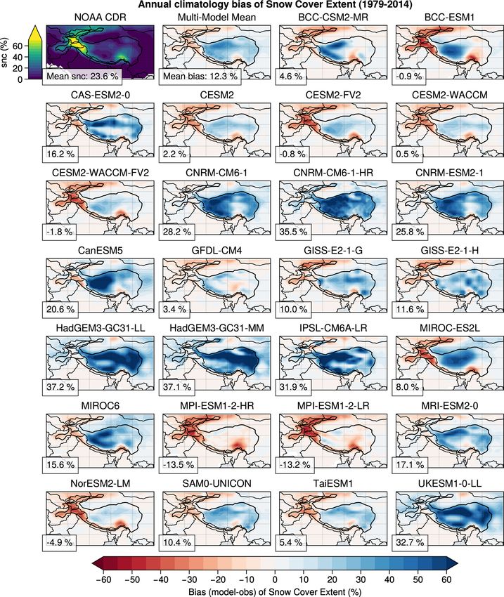
1062                                                  M. Lalande et al.: Climate change in the High Mountain Asia in CMIP6

1   Introduction                                                  over the TP, depending on the location and the period (Kang
                                                                  et al., 2010). Increasing temperature induced a reduction of
High Mountain Asia (HMA) extends from the Himalayas in            the snow cover fraction in HMA, but this has been com-
the south and east to the Hindu Kush in the west and to Tien      pensated by an increase in precipitation leading to stronger
Shan in the north, including also the Karakoram, the Pamir-       snowfall rates in some regions (Viste and Sorteberg, 2015;
Alay and the Kunlun mountain ranges. HMA surrounds the            Notarnicola, 2020). Upon its impact on snow cover, climate
Tibetan Plateau (TP), which is the highest and most exten-        change in HMA and TP affects also the permafrost and the
sive plateau in the world, with an average elevation of 4000 m    glaciers (Yang et al., 2010; Yao et al., 2007), increases the
above sea level and an approximate surface area of 2.5 mil-       desertification (Xue et al., 2009) and affects the hydrological
lion km2 (Du and Qingsong, 2000). Because of their high el-       cycle inducing serious threats for the water resources used for
evation and complex terrain, TP and HMA affect not only           agriculture, drinking water and hydroelectricity (Qiu, 2008;
the regional climate and environment in East Asia but also        Immerzeel et al., 2010; Sabin et al., 2020). HMA is also fac-
the global atmospheric circulation via thermal and mechan-        ing an increase in both the intensity and the frequency of
ical forcings (Flohn, 1957; Kutzbach et al., 1993; Webster        heatwaves (Ding et al., 2018). The lack of observations, es-
et al., 1998; Hsu and Liu, 2003; Duan and Wu, 2005; Liu           pecially pronounced in the western part of HMA, limits the
et al., 2007; Wu et al., 2016). The Asian summer monsoon          possibility to understand and anticipate the climate change in
provides almost 80 % of the annual precipitation in the cen-      this area (Orsolini et al., 2019).
tral and eastern parts of the Himalayas during the monsoon           Current coupled ocean–atmosphere general circulation
season (June–September) (Bookhagen and Burbank, 2010;             models (GCMs) have a overly coarse spatial resolution (from
Palazzi et al., 2013; Sabin et al., 2020). Several studies sug-   50 km to several hundred kilometers) to reproduce the small-
gested that the geographical configuration of the TP was en-      scale variability of temperature, precipitation and snow cover
hancing the triggering of the Asian monsoon, with this dry        that is observed over complex topography areas. Neverthe-
area acting as a heat source transferred to the midtroposphere    less, they may be effective in providing a smooth but consis-
directly enhancing the vertical uplift typically found at the     tent picture of the large-scale temporal and spatial patterns
start of the summer monsoon (Li and Yanai, 1996; Wu and           of these key variables at the regional scale. The Coupled
Zhang, 1998; Yihui and Chan, 2005; Wu et al., 2012). This         Model Intercomparison Project (CMIP) organized by the
finding has been partly questioned in other studies, suggest-     World Climate Research Programme (WCRP), recently dis-
ing that the Himalayan chain is insulating the warm and           tributed under its sixth phase (CMIP6) (Eyring et al., 2016),
moist air found over the Indian subcontinent from the cold        is a unique opportunity to conduct comprehensive analyses
areas found in TP (Boos and Kuang, 2010). Therefore, the          of the climate variability and change at both global and re-
Himalayas and not the TP seem to be an essential geograph-        gional scales, based on an ensemble of climate models.
ical feature that favors vertical uplifts of warm and moist air      GCM experiments show generally good skill for sur-
masses, mainly on their southern flank. In contrast, winter       face temperature; however, a systematic cold bias over TP
precipitation contributes nearly half of the annual precipi-      and mountainous areas has been pointed in GCM outputs
tation in the Karakoram and the Hindu Kush, mostly due            since the first Atmospheric Model Intercomparison Project
to the westerly disturbances (WDs) bringing moisture from         (AMIP) experiments (Mao and Robock, 1998). Su et al.
the Atlantic Ocean, and the Mediterranean and Caspian seas        (2013) showed that most of the CMIP5 models have a cold
(Singh et al., 1995; Vandenberghe et al., 2006; Palazzi et al.,   bias at the surface in the eastern TP, with a mean underesti-
2013; Kapnick et al., 2014; Madhura et al., 2015; Cannon          mation of −1.1 to −2.5 ◦ C over December to May, and less
et al., 2015; Hunt et al., 2018; Krishnan et al., 2019). TP and   than −1 ◦ C over June to October in comparison to ground
HMA are often referred as the “Asian Water Tower” and/or          observations, while the annual climatology of precipitation
the “Third Pole” (e.g., Immerzeel et al., 2010; Qiu, 2008; Yao    is overestimated by 62 % to 183 %. Regional climate models
et al., 2012, 2019) because they are the largest freshwater re-   show similar cold biases, a deficiency that is often associated
source stored in the cryosphere after the polar ice sheets. In    with an excess of precipitation in the experiments (Lee and
this region, snowmelt ensures a permanent water flow to the       Suh, 2000). However, the lack of high-elevation observation
major Asian river systems, such as the Yangtze, Yellow, Sal-      station data may also be partly responsible for the apparent
ween and Mekong rivers (Sharma et al., 2019), contributing        cold bias of the model (Gu et al., 2012), and high-resolution
to the water supply of over 1.4 billion people living down-       experiments suggest that the real precipitation rates occur-
stream (Immerzeel and Bierkens, 2012; Yao et al., 2012; Ra-       ring at high elevation are likely stronger than those estimated
sul, 2014; Scott et al., 2019; Wester et al., 2019).              from gridded products based on rain gauge measurements
   Over 1955–1996, Liu and Chen (2000) estimated an an-           (Dimri et al., 2013). GCMs show cold biases also at 500 hPa,
nual warming rate over the TP of 0.16 ◦ C decade−1 that           which may be caused by penetration of dry and cold air from
reached 0.32 ◦ C decade−1 in winter, while Wang et al. (2008)     the deserts of western Asia due to an overly smoothed rep-
observed an annual warming of 0.36 ◦ C decade−1 over 1960–        resentation of topography west of the TP (Boos and Hurley,
2007. Precipitation and snow cover show contrasted trends         2013; Xu et al., 2017). Chen et al. (2017) suggested that im-

Earth Syst. Dynam., 12, 1061–1098, 2021                                            https://doi.org/10.5194/esd-12-1061-2021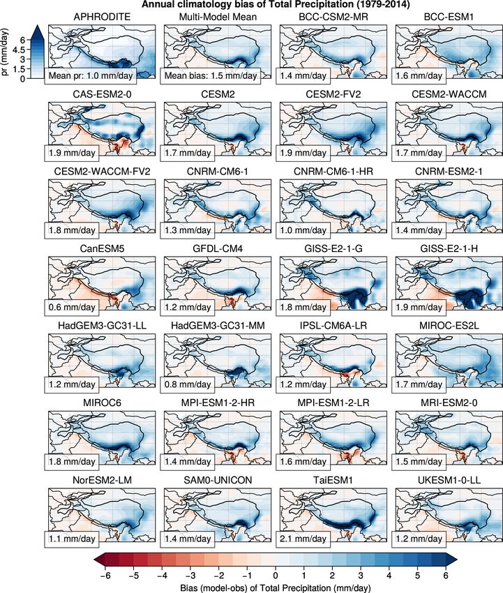
M. Lalande et al.: Climate change in the High Mountain Asia in CMIP6                                                       1063

provements in the parameterization of snow cover area and         by the modeling group (Table A1). The version of the model
boundary layer processes in CMIP5 models should allow to          data is the most recent one available at the time of this anal-
improve the representation of the surface energy budget and       ysis.
to reduce the cold bias over TP. Model biases are also re-
lated to inaccurate descriptions of the elevation and the at-     2.2     Observations
mospheric circulation as the Asian anticyclone or summer
monsoon (e.g., Salunke et al., 2019; Duan et al., 2013). More     Because of complex topography, severe weather and harsh
recently, Zhu and Yang (2020) compared CMIP6 and CMIP5            environmental conditions in HMA and TP, meteorological
models over 1961–2014 to finally conclude that the cold bias      observations are rare in this region. Available weather sta-
and the wet bias over TP, even if reduced, still persist in the   tions are usually sparse and unevenly distributed (Wang and
most recent version of these models.                              Zeng, 2012; Su et al., 2013). Gridded data, satellite obser-
   Our study focuses on the climate variability over HMA as       vations and reanalyses are combined here to obtain a robust
simulated with CMIP6 models. The near-surface air temper-         evaluation of model biases, even if they are affected by the
ature, the snow cover extent and the total precipitation are      uncertainties inherent to the observations.
considered to answer four questions: (1) what are the biases
in HMA in this new generation of climate models for these         2.2.1    Near-surface air temperature
three variables? (2) What are the links between the model bi-
ases in temperature, precipitation and snow cover? (3) Do the     The CRU TS (Climatic Research Unit gridded Time Series)
model biases impact the simulated climate trends? (4) Which       version 4.00 (https://doi.org/10/gbr3nj) provides a 0.5◦ grid-
climate projections can be expected in this area over the next    ded dataset of the monthly temperature (excluding Antarc-
century? The datasets and methods used in this study are de-      tica) available from 1901 until the present, based on local
scribed in the next section. Section 3 presents a comparison      weather stations and provided with an estimation of the data
between observations and 26 CMIP6 models over the histor-         quality (Harris et al., 2020). This dataset has been widely
ical period with a focus on the potential correlations between    used over HMA and TP (e.g., Gu et al., 2012; Chen et al.,
the biases of the different variables. We then show the histor-   2017; Krishnan et al., 2019; Wang et al., 2021; Yi et al.,
ical trends estimated from the CMIP6 experiments and their        2021). Correlation with local measurements, including at
potential dependency on model biases (Sect. 4). Section 5         high elevation (Wang et al., 2013b), is high in this region.
explores future projections under different scenarios cover-      This gives confidence for model evaluation (Chen et al.,
ing the 21st century. The results are discussed in Sect. 6 and    2017).
the conclusions are presented in Sect. 7.
                                                                  2.2.2    Snow cover extent
2     Data and methods
                                                                  In situ snow observations are sparse over HMA and
2.1    Models
                                                                  TP, and when they are available, in situ data are of-
                                                                  ten not representative for snow cover analysis at the
In this study, we selected 26 GCMs Table 1 in the CMIP6           regional scale (Gurung et al., 2017). Alternatively, re-
database (Eyring et al., 2016) focusing on near-surface air       mote sensing datasets provide large-scale snow informa-
temperature (tas), total precipitation (pr) and snow cover ex-    tion useful for spatiotemporal analyses. The satellite prod-
tent (snc) over 1979–2014. Only 10 of these models are            uct available over the longest period, but at a coarse spa-
available for future projections covering the ensemble of         tial resolution, is the NOAA Climate Data Record (CDR)
the SSP1-2.6, SSP2-4.5, SSP3-7.0 and SSP5-8.5 Shared So-          (Robinson et al., 1993, 2012; Estilow et al., 2015), covering
cioeconomic Pathways, which are combining socioeconomic           the Northern Hemisphere (NH) from 4 October 1966 to
scenarios and radiative forcing levels (O’Neill et al., 2016).    present (referred to as NOAA CDR in this article). Data
Considering the model uncertainties, such a limited number        prior to June 1999 are based on weekly satellite-derived maps
of models might be sufficient to explore future climate trends    of snow cover extent, whereas posterior data have been re-
(Knutti et al., 2010). The resolution of the models ranges        placed by daily snow cover extent estimated from the Interac-
from about 3 to 0.5◦ (∼ 300 to 50 km), while most of them         tive Multisensor Snow and Ice Mapping System (IMS). The
reach a 1◦ resolution. All models are regridded on a common       weekly snow cover extent maps are digitized to a 88×88 grid
1◦ × 1◦ grid using a bilinear interpolation before the multi-     following a 190 km polar stereographic projection and con-
model analysis.                                                   tain binary snow cover information. The retrieval of snow
   Climatologies are computed with the first member (usu-         cover information for this product is not interfered by clouds
ally r1i1p1f1), whereas trend analyses are based on ensemble      due to the weekly aggregation prior to June 1999 and the
means for each model, restricted to a single setup of physi-      inclusion of passive microwave data posterior. The NOAA
cal parameterization (p), initialization method (i) and forc-     CDR has been widely used in climate–snow studies over the
ing (f ), except when a different recommendation is given         NH (e.g., Brown and Robinson, 2011; Hernández-Henríquez

https://doi.org/10.5194/esd-12-1061-2021                                          Earth Syst. Dynam., 12, 1061–1098, 2021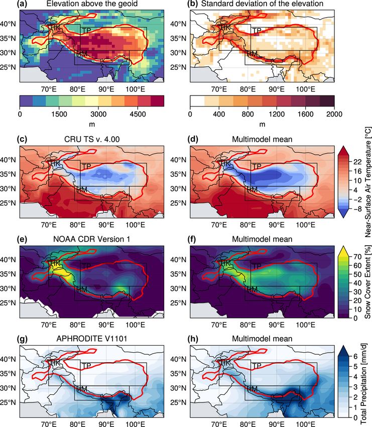
1064                                                       M. Lalande et al.: Climate change in the High Mountain Asia in CMIP6

Table 1. Description of the CMIP6 models used in this study with their institute, name, approximate spatial resolution (longitude × latitude),
the member considered in the one-member analyses and their reference. A cross is included in the last column when the model projections
are available for the four SSP scenarios (SSP1-2.6, SSP2-4.5, SSP3-7.0 and SSP5-8.5).

 Institute (country)          Model                    Resolution     Primary    All SSPs    Reference
                                                       (long × lat)   member     available
                              BCC-CSM2-MR              1.1◦ × 1.1◦                  ×        Wu et al. (2018); Xin et al. (2019)
 BCC (China)                                                          r1i1p1f1
                              BCC-ESM1                 2.8◦ × 2.8◦                           Zhang et al. (2018a)
 CAS (China)                  CAS-ESM2-0               1.4◦ × 1.4◦    r4i1p1f1               Chai (2020)
                              CESM2                    1.2◦ × 0.9◦                           Danabasoglu (2019a)
                              CESM2-FV2                2.5◦ × 1.9◦                           Danabasoglu (2019b)
 NCAR (USA)                                                           r1i1p1f1
                              CESM2-WACCM              1.2◦ × 0.9◦                           Danabasoglu (2019c)
                              CESM2-WACCM-FV2          2.5◦ × 1.9◦                           Danabasoglu (2019d)
                              CNRM-CM6-1               1.4◦ × 1.4◦                           Voldoire (2018, 2019a)
 CNRM-CERFACS (France)        CNRM-CM6-1-HR            0.5◦ × 0.5◦    r1i1p1f2      ×        Voldoire (2019b, c)
                              CNRM-ESM2-1              1.4◦ × 1.4◦                           Seferian (2018, 2019)
 CCCma (Canada)               CanESM5                  2.8◦ × 2.8◦    r3i1p2f1      ×        Swart (2019a, b)
 NOAA-GFDL (USA)              GFDL-CM4                 1.2◦ × 1.0◦    r1i1p1f1               Guo et al. (2018)
                              GISS-E2-1-G                                                    NASA Goddard Institute for Space Studies (2018)
 NASA-GISS (USA)                                       2.5◦ × 2.0◦    r1i1p1f1
                              GISS-E2-1-H                                                    NASA Goddard Institute for Space Studies (2019)
                              HadGEM3-GC31-LL          1.9◦ × 1.2◦                           Ridley et al. (2019a)
 MOHC (UK)                                                            r1i1p1f3
                              HadGEM3-GC31-MM          0.8◦ × 0.6◦                           Ridley et al. (2019b)
 IPSL (France)                IPSL-CM6A-LR             2.5◦ × 1.3◦    r1i1p1f1      ×        Boucher et al. (2018, 2019)
                              MIROC-ES2L               2.8◦ × 2.8◦    r1i1p1f2               Hajima et al. (2019); Tachiiri et al. (2019)
 MIROC (Japan)                                                                      ×
                              MIROC6                   1.4◦ × 1.4◦    r1i1p1f1               Tatebe and Watanabe (2018); Shiogama et al. (2019)
                              MPI-ESM1-2-HR            0.9◦ × 0.9◦                           Jungclaus et al. (2019)
 MPI-M (Germany)                                                      r1i1p1f1
                              MPI-ESM1-2-LR            1.9◦ × 1.9◦                           Wieners et al. (2019)
 MRI (Japan)                  MRI-ESM2-0               1.1◦ × 1.1◦    r1i1p1f1      ×        Yukimoto et al. (2019a, b)
 NCC (Norway)                 NorESM2-LM               2.5◦ × 1.9◦    r2i1p1f1               Seland et al. (2019)
 SNU (South Korea)            SAM0-UNICON              1.2◦ × 0.9◦    r1i1p1f1               Park and Shin (2019)
 AS-RCEC (Taiwan)             TaiESM1                  1.2◦ × 0.9◦    r1i1p1f1               Lee and Liang (2020)
 MOHC (UK)                    UKESM1-0-LL              1.9◦ × 1.2◦    r1i1p1f2      ×        Tang et al. (2019); Good et al. (2019)

et al., 2015; Hori et al., 2017; Santolaria-Otín and Zolina,              et al., 2021). It covers the period 1982–2020 at a daily
2020) and more specifically over HMA (e.g., Xu et al.,                    temporal and 0.05◦ spatial resolution. The product is
2016). This dataset is adapted for continental-scale studies              based on the Fundamental Climate Data Record (FCDR)
but shows limitations over mountainous regions (Déry and                  consisting of daily composites of AVHRR GAC data
Brown, 2007), even if the inclusion of Meteosat-5 data in                 (https://doi.org/10.5676/DWD/ESA_Cloud_cci/AVHRR-
2001 significantly improved its quality over the Asian conti-             PM/V003) produced in the ESA Cloud CCI project (Stengel
nent (Helfrich et al., 2007). Trend analyses based on NOAA                et al., 2020). The data were pre-processed with an improved
CDR data must be taken with caution because of potential                  geocoding and an inter-channel and inter-sensor calibration
temporal heterogeneities related to changes of experimen-                 using PyGAC (Devasthale et al., 2017). Alongside the
tal protocols (Mudryk et al., 2020). To obtain monthly frac-              daily reflectance and brightness temperature information,
tional values, we simply average the weekly binaries values               an excellent cloud mask including pixel-based uncertainty
included in each corresponding month.                                     information is provided (Stengel et al., 2017, 2020). Snow
   The Advanced Very High Resolution Radiometer                           cover extent was retrieved using SCAmod (Metsämäki
(AVHRR) Global Area Coverage (GAC) snow cover                             et al., 2015), while water bodies, permanent ice bodies and
extent time series version 1 derived in the frame of                      missing values are flagged. To reduce the effect of cloud
the European Space Agency’s Climate Change Ini-                           coverage, a temporal filter of ±3 d of each individual snow
tiative (ESA CCI+) Snow project is the most recent                        cover observation was applied after Foppa and Seiz (2012).
long-term global snow cover product available (Naegeli                    The AVHRR GAC FCDR snow cover product comprises

Earth Syst. Dynam., 12, 1061–1098, 2021                                                       https://doi.org/10.5194/esd-12-1061-2021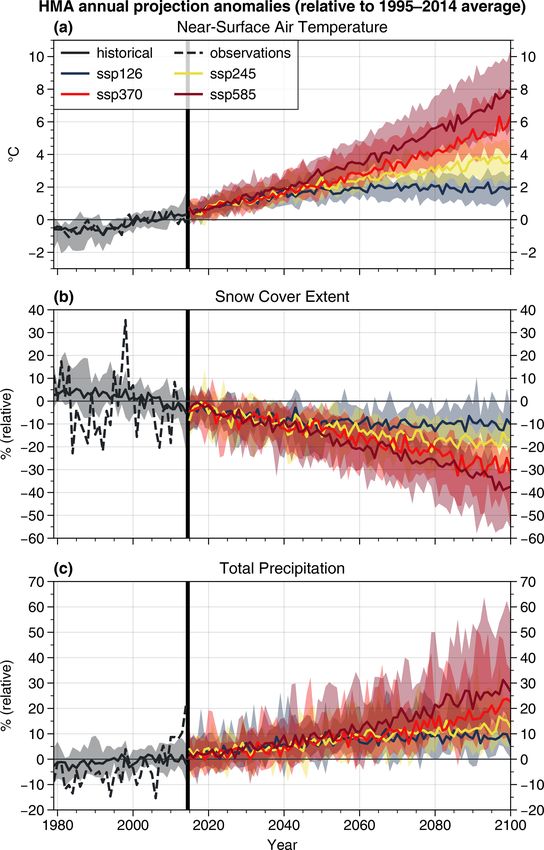
M. Lalande et al.: Climate change in the High Mountain Asia in CMIP6                                                        1065

only one longer data gap of 92 d between November 1994             ing separately the rainfall and snowfall rates (Palazzi et al.,
and January 1995, resulting in a 99 % data coverage over the       2013). However, climate trends estimated from reanalysis
entire study period of 38 years. For the computation of the        data are affected by the continuous changes in the observ-
average annual cycle over the study period, the permanent          ing systems that can introduce spurious variability and trends
ice bodies were assumed to be 100 % snow covered, whereas          (Bengtsson, 2004). Global atmospheric reanalyses show poor
water bodies, remaining clouds or other missing values             quality over HMA and TP also because of their coarse res-
were not taken into account. Due to the slightly shorter time      olution and the limited number of local observations avail-
period covered by this snow product compared to the period         able for the assimilation process that is not adapted for such
investigated in this study, it was not considered for trend        complex topography areas (You et al., 2010; Norris et al.,
analysis.                                                          2015, 2017).

2.2.3    Precipitation                                             2.3.1   ERA-Interim

In this study, we use the daily APHRODITE (Asian                   ERA-Interim is a global atmospheric reanalysis dataset pro-
Precipitation-Highly-Resolved Observational Data Integra-          duced by the European Centre for Medium-Range Weather
tion Towards Evaluation of Water Resources) product (Yata-         Forecasts (ECMWF), covering the period from 1979 to 2019
gai et al., 2012) version V1101 (1951–2007) and its ex-            at approximately 80 km on 60 vertical levels (Dee et al.,
tended version V1101EX_R1 (2007–2015) over the domain              2011). ERA-Interim shows best overall performance for air
of monsoon Asia (MA) at a 0.5◦ resolution. APHRODITE               temperatures compared to other reanalyses over TP (Wang
includes a large number of local observations and includes         and Zeng, 2012) and high correlations (0.97 to 0.99) with
a correction in the interpolation process for complex topog-       respect to ground meteorological stations during 1979–2010
raphy areas. The seasonal precipitation is correctly repre-        (Gao et al., 2014). Estimates of precipitation associated with
sented in APHRODITE (e.g., Palazzi et al., 2013; Kapnick           the reanalysis are produced by the forecast model, based on
et al., 2014). However, most of the stations are located in        the assimilation of temperature and humidity observations
the eastern and southern parts of the TP and do not cover          (Palazzi et al., 2013). Snow depth is assimilated through
the high-elevation areas. For comparison, we used the Global       station observations (Orsolini et al., 2019), and gridded
Precipitation Climatology Project (GPCP) CDR version 2.3           snow cover from IMS has also been assimilated since 2004
(monthly) product at 2.5◦ (Adler et al., 2016, 2018). This         (Drusch et al., 2004). As described in the ECMWF docu-
product combines satellite products with rain gauge stations       mentation (https://confluence.ecmwf.int/display/CKB/ERA-
available from 1979 to the present. However, the scarcity          Interim:+documentation#ERAInterim:documentation-
of high-elevation in situ stations, the interference of wind       Computationofnear-surfacehumidityandsnowcover,             last
with the sensors and the problems of satellite-based meteo-        access: 13 October 2021), snow cover fraction (SCF) is
rological radars in identifying snow crystals lead to large un-    a diagnostic variable computed directly using snow water
certainties in observational snowfall datasets (Palazzi et al.,    equivalent (i.e., parameter SD in meters of water equivalent)
2013; Sun et al., 2018). Total precipitation is therefore gener-   as SCF = min(1, RW × SD/15), where RW is the density of
ally underestimated, especially over snow-rich areas (Sanjay       water equal to 1000.
et al., 2017).
                                                                   2.3.2   ERA5
2.2.4    Topography                                                ERA5 is the most recent global atmospheric reanalysis pro-
                                                                   duced by the ECMWF and replaces ERA-Interim (Hersbach
Global Multi-resolution Terrain Elevation Data 2010
                                                                   et al., 2020). The improvements, including the spatial and
(GMTED2010) (Danielson and Gesch, 2011) (available at
                                                                   temporal resolution (hourly estimates at 31 km distributed
https://www.temis.nl/data/gmted2010/index.php, last access:
                                                                   on 137 levels), allowed for example an improved represen-
1 June 2021) provide elevations and its standard deviation at
                                                                   tation of the troposphere and better global balance of pre-
multiple resolutions and are realistic over HMA (Grohmann,
                                                                   cipitation and evaporation. As in ERA-Interim, snow cover
2016). In this study, we use the 1◦ × 1◦ resolution as a refer-
                                                                   fraction is a diagnostic variable that can be computed from
ence grid.
                                                                   snow water equivalent (i.e., parameter SD in meters of water
                                                                   equivalent) and snow density (i.e., RSN in kg m−3 ) as SCF =
2.3     Reanalyses                                                 min(1, (RW × SD/RSN)/0.1), where RW is the density of
                                                                   water equal to 1000. Unlike ERA-Interim, IMS data are not
Reanalysis data, based on assimilation of meteorological
                                                                   used above 1500 m, i.e., in high-altitude regions which in-
observations, provide an estimate of the climate variabil-
                                                                   clude the TP (ECMWF, 2020a).
ity at the global and regional scales consistent with the ob-
served variability. An advantage over most observations is
that reanalysis data do account for total precipitation, provid-

https://doi.org/10.5194/esd-12-1061-2021                                           Earth Syst. Dynam., 12, 1061–1098, 2021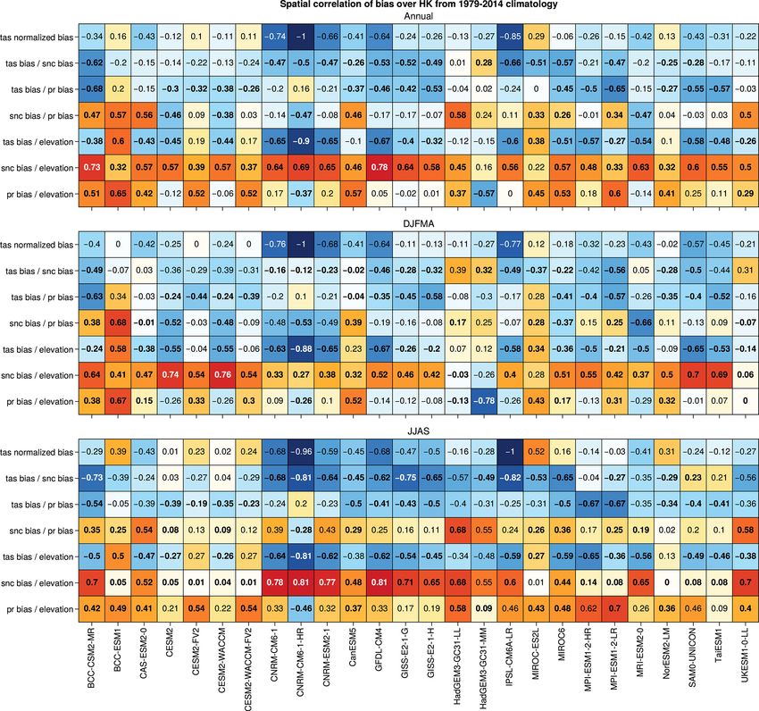
1066                                                    M. Lalande et al.: Climate change in the High Mountain Asia in CMIP6

2.4    Study area                                                      For model evaluation, we use two different metrics based
                                                                    on spatial climatologies: the root mean square error (RMSE;
In this study, we consider HMA as a box covering 20–45◦ N           Eq. 1) and the mean bias (Eq. 2), which we slightly modified
and 60–110◦ E (Fig. 1a and b), focusing on mountain areas,          to take into account the spatial weight (w; Eq. 3) of each grid
including the TP, with an elevation higher than 2500 m. As          cell.
in previous studies considering different climatic areas (e.g.,
                                                                               v
Palazzi et al., 2013; Kapnick et al., 2014; Sanjay et al., 2017),              u             n
                                                                                     1      X
                                                                                                wi (Mi − Oi )2
                                                                               u
three subdomains are considered: Hindu Kush–Karakoram               RMSE = t Pn                                                 (1)
(HK; 31–40◦ N, 70–81◦ E), Himalayas (HM; 26–31◦ N, 79–                              i=1 w i i=1
98◦ E) and the Tibetan Plateau (TP; 31–39◦ N, 81–104◦ E)                                   n
                                                                                  1        X
using grid cells within each subregion above 2500 m. HK is          Mean bias = Pn                wi (Mi − Oi )                (2)
largely influenced by WDs, whereas most of the precipitation                         i=1 wi i=1
over HM is related to the Asian summer monsoon. A cold              w = cos λ,                                                 (3)
and dry continental climate is found in TP (Bookhagen and
Burbank, 2010; Palazzi et al., 2013; Sabin et al., 2020).           where λ is the latitude, Mi represents model simulations, and
                                                                    Oi is the observed data.
                                                                       To characterize the multimodel ensemble, mean or median
2.5    Numerical methods and computations                           are usually considered in addition to their 5th and 95th per-
Trend computations are based on linear least-squares re-            centiles (e.g., mean/median [5th, 95th]). A multimodel mean
gression. We consider a 95 % level of significance, cor-            is used in bias analysis, and projections are based on the mul-
responding to a p value equal to 0.05, computed with a              timodel median.
two-sided Wald test for which the null hypothesis corre-
sponds to a slope equal to zero (https://docs.scipy.org/doc/        3     Historical bias analysis
scipy/reference/generated/scipy.stats.linregress.html, last ac-
cess: 22 July 2021). The linear relationship between two            Model biases are computed with the CRU, APHRODITE
datasets is estimated with the Pearson correlation coefficient.     and NOAA CDR observation datasets used as references
   We consider a 95 % level of significance, correspond-            for near-surface air temperature, total precipitation and snow
ing to a p value equal to 0.05, computed as follows: for            cover extent, respectively, over the period 1979–2014. To get
a given sample with correlation coefficient r, the p value          confidence in the model bias quantification, we use further
is the probability that |r0| of a random sample x0 and y0           observational datasets, including GPCP precipitation, ESA
drawn from the population with zero correlation would               CCI snow cover as well as ERA-Interim and ERA5 reanaly-
be greater than or equal to |r| (https://docs.scipy.org/doc/        sis.
scipy/reference/generated/scipy.stats.pearsonr.html, last ac-
cess: 22 July 2021). Note that the spatial correlation asso-        3.1    Climatologies
ciated with p values in Figs. 4 and C1–C3 does not include
any dependency on the cell area. This arbitrary choice im-          The annual climatology computed over 1979–2014 is shown
plies that the models are evaluated grid cell by grid cell and      in Fig. 1 for the CRU, NOAA CDR and APHRODITE ob-
not per unit of surface. However, the impact on the spatial         servations (panels c, e, g) and the multimodel mean based
correlation is minor in our case, given that HMA is a rela-         on 26 CMIP6 models (panels d, f, h). Over HMA, temper-
tively small area including model grid cells with areas that        ature ranges from −8 ◦ C in high-elevation areas to 13 ◦ C at
are relatively similar.                                             lower elevation in observations with an average of −0.2 ◦ C
   The cosine latitude is taken into account as a weight in         (Fig. 1c). HMA temperature reaches −15 to 9 ◦ C in winter
spatial averages and the exact number of days in each month,        and 2 ◦ C to 19 ◦ C in summer (not shown). The multimodel
depending on the calendar type, is considered in temporal av-       mean shows colder temperatures than observations, with val-
erages. Our analyses cover the historical period 1979–2014          ues ranging from −11 to 3 ◦ C and a mean value over HMA
and projections over 2015–2100, focusing on two seasons:            about −2.1 ◦ C (Fig. 1d). Even with a general cold bias, the
the summer extending from June to September (JJAS), a pe-           spatial pattern of temperature in the model is consistent with
riod when the monsoon is active (Palazzi et al., 2013; Sabin        the observations, with a spatial correlation of 0.87.
et al., 2013), and the winter defined as the months covering           Snow cover extent is heterogenous over HMA (Fig. 1e),
December to April (DJFMA), a period affected by WD pre-             with high values over HK reaching more than 70 %, which
cipitation especially pronounced over the Hindu Kush and            are explained by strong winter snowfalls related to WDs
Karakoram areas (Palazzi et al., 2013; Kapnick et al., 2014;        (Cannon et al., 2015; Bao and You, 2019). Snow cover extent
Cannon et al., 2015; Hunt et al., 2018; Krishnan et al., 2019).     is much smaller over most of the TP region, with annual val-
Annual means are also considered when the seasonal analy-           ues not exceeding 20 %. High values, around 50 %, are also
sis does not show additional information.                           found over Tien Shan and the southeastern Himalayas. In the

Earth Syst. Dynam., 12, 1061–1098, 2021                                              https://doi.org/10.5194/esd-12-1061-2021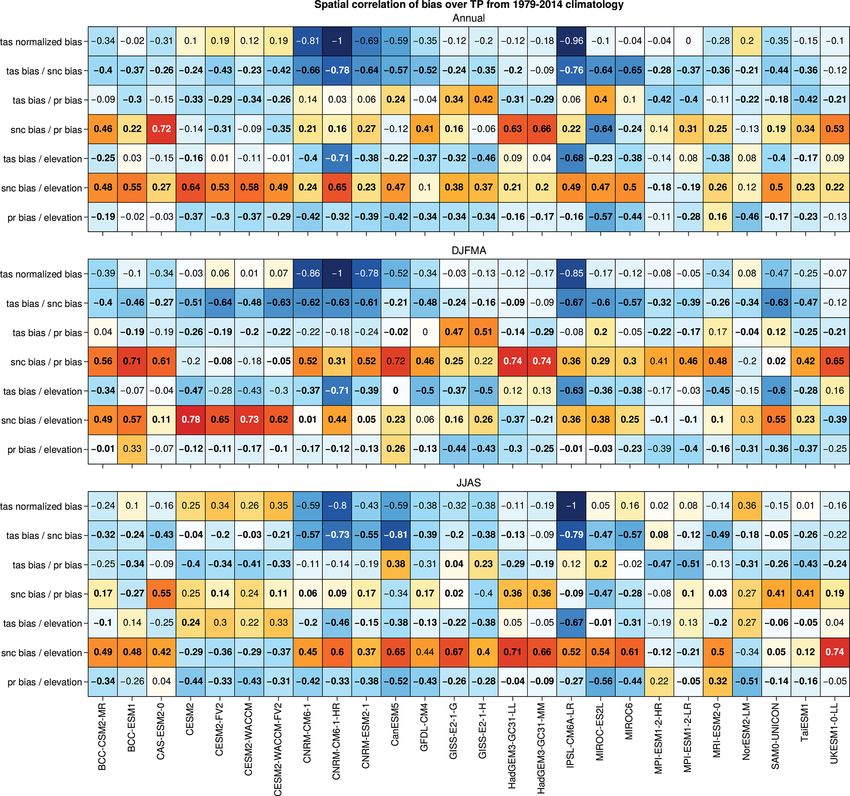
M. Lalande et al.: Climate change in the High Mountain Asia in CMIP6                                                                1067

Figure 1. Surface elevation (a) and its standard deviation (b) estimated from GMTED2010 at 1◦ . Annual climatologies computed over
1979–2014 for temperature (c, d), snow cover (e, f) and precipitation (g, h); the left panels correspond to the observations from CRU (c),
NOAA CDR (e), and APHRODITE (g), while the right panels (d, f, h) correspond to the multimodel mean (using the first realization of
each ensemble model). The red contour highlights the HMA domain limited to areas higher than 2500 m a.s.l., and the black boxes define
the subdomains Hindu Kush–Karakoram (HK), Himalayas (HM), and the Tibetan Plateau (TP), which are also limited to areas higher than
2500 m a.s.l. (red contour) in this study.

multimodel mean (Fig. 1f), snow cover is overestimated over            of snow cover in this area (Fig. 1e). Due to the orographic
most of the TP and slightly underestimated over the HK re-             barrier, the TP located more on the east is much drier, with
gion in comparison with the observations.                              annual mean precipitation generally lower than 1 mm d−1 .
   Strong precipitation rates, reaching an annual mean of              The multimodel mean (Fig. 1h) shows globally higher values
more than 6 mm d−1 (exceeding 2000 mm yr−1 ), are observed             of precipitation over HMA in comparison with the observa-
in the eastern part of HM, mostly due to the Asian summer              tions. Precipitation tends to spread more over the TP in the
monsoon, with a decreasing influence from the southeast to             model compared to the observations, which might be partly
the northwest Himalayan chain (Fig. 1g). In contrast, the HK           due to the smoothing of the topography in the models. How-
region receives moisture from both Asian summer monsoon                ever, precipitation rates are also generally underestimated in
and WDs (Fig. 2j). Moisture-laden westerly winds are inter-            observational datasets because of snowfall undercatch issues,
cepted by high mountain ranges in northern Pakistan, lead-             which could lend credence in the stronger precipitation rates
ing to moisture condensation and precipitation at high eleva-          modeled at high elevation.
tion (Palazzi et al., 2013), partly explaining the high values

https://doi.org/10.5194/esd-12-1061-2021                                                 Earth Syst. Dynam., 12, 1061–1098, 2021
1068                                                     M. Lalande et al.: Climate change in the High Mountain Asia in CMIP6

3.2    Temperature, snow cover and precipitation annual              estimation of snow cover that is comparable to the CMIP6
       cycle                                                         model ones. This behavior has already been described in Or-
                                                                     solini et al. (2019), explaining this difference by the fact that
The seasonal cycles are shown in Fig. 2 for the models and           ERA5 does not assimilate IMS data beyond 1500 m a.s.l.,
different observational datasets and reanalyses over HMA             while Hersbach et al. (2020) suggests that the single-layer
and the three subdomains for temperature, snow cover and             snow scheme does not allow enough melting in mountainous
precipitation. The model biases with respect to observations         regions. The differences found over the three subdomains are
are stronger in winter than in summer for temperature and            similar to those highlighted over the whole HMA (Fig. 2f–h).
snow cover, a feature already noticed in CMIP5 and CMIP6             Nevertheless, we note a precocious spring melt in the multi-
(e.g., Su et al., 2013; Zhu and Yang, 2020). Indeed, the multi-      model mean and ERA-Interim compared to the NOAA CDR
model mean temperature is around 2 to 3 ◦ C below the CRU            observations and ERA5 in HK region (Fig. 2f). The ESA CCI
observations in winter over HMA, while models and obser-             product shows lower snow cover values compared to NOAA
vations are much closer in summer (Fig. 2a). These differ-           CDR and ERA-Interim, with values around 30 % during the
ences are more pronounced in the HK region (Fig. 2b) with            winter in HMA, suggesting that model biases may be even
differences noticed both in winter (4 to 5 ◦ C) and summer           larger. The large difference in spatial resolution with the lat-
(∼2 ◦ C). The cold bias appears in the multimodel mean (dark         ter product may also play a role in this discrepancy, as valleys
blue line) from October/November onwards, peaks between              and other aspects of fine-scale topography are not being well
December and January, and then decreases until April/May,            resolved in the other products and thus lack a good represen-
except in the HK area where the bias persists in summer.             tation of the spatial heterogeneity of snow cover compared
Nevertheless, the multimodel spread encompasses the ob-              to the ESA CCI product. This suggests a general snow cover
servation and reanalyses datasets, suggesting a certain reli-        overestimation in both model and reanalysis data based on
ability of the CMIP6 models. This spread, denoted with the           coarse resolution, which is especially pronounced over high
confidence intervals at 50 % and 90 % of the multimodel en-          mountain areas (Fig. 2f, g). Nevertheless, the positive bias
semble (dark and light shadings), highlights a higher disper-        of snow cover fraction simulated by the models over HMA
sion between the models in winter than in summer, except             is mainly related to the overestimation of the snow cover
for the HK region. It can be assumed that the larger biases in       over TP, where the snow cover varies around 20 % for the
winter may be due to excessive snowfall, leading to larger           observations, while values above 60 % are found in the mul-
snow cover which can amplify the phenomenon. Further-                timodel mean, despite a wide dispersion among the models
more, due to the poor representation of fine-scale topography,       (from 20 % to 90 %).
one can assume that most of the moisture fluxes condense                The strongest precipitation rates occur during the Asian
on the plateau at higher elevations, favoring snow precipita-        summer monsoon over the HM region (> 2500 m), with
tion, instead of precipitating earlier on the mountainside. The      precipitation rates reaching a monthly mean of 10 mm d−1
greater difference in the HK region can be supported by this         (∼ 300 mm month−1 ) on average in the multimodel mean,
later hypothesis, knowing that this area is particularly subject     while precipitation rates reach lower values than 2 mm d−1
to winter WDs bringing a large amount of snow precipitation          during the winter (Fig. 2k). Other regions exhibit smaller pre-
on the reliefs. Alternatively, it may also be due to the fact that   cipitation amounts below 5 mm d−1 most of the year. In the
there are very few weather stations in this area, especially at      HK region, larger precipitation rates are found in late win-
high elevation, and therefore the interpolated CRU data may          ter and spring (Fig. 2j) mostly due to WDs, as explained in
be overestimated compared to the actual values (Gu et al.,           Sect. 1. While the model spread generally encompasses the
2012). More details on the possible links between the biases         observations for temperature and snow cover, APHRODITE
are explored in Sect. 3.4.                                           precipitation data are most of the time below the minimum
   In comparison with the NOAA CDR satellite observation,            of the model values. This difference might be explained by
the multimodel mean snow cover over HMA is overestimated             snow undercatch issues typically obtained with rain gauge
by 20 % in winter and is closer to the observations in sum-          measurements (e.g., Jimeno-Sáez et al., 2020), whereas mod-
mer when snow cover is lowest (Fig. 2e). The model spread is         els are expected to provide both solid and liquid precipita-
larger for snow cover than for temperature and precipitation,        tion. In addition, rain gauge measurements are generally too
with values varying from 20 % to 90 % in winter and 0 % to           sparse to estimate the heterogeneous distribution of precip-
40 % in summer. This large spread highlights the difficulty to       itation over complex topography areas. Over HK, a large
simulate snow cover in complex topography areas and also             part of the precipitation falls as snow in winter, a period
the large internal variability of snow cover. ERA-Interim is         when strong differences between satellite/rain gauge prod-
again very close to the observations for snow cover, likely          ucts (black curves) and models/reanalyses are also appear-
because of the assimilation of IMS data in this reanalysis,          ing during February to May, whereas the precipitation is
a satellite product also used in the production of the NOAA          closer between models and observations during the summer
CDR dataset (Drusch et al., 2004; Robinson et al., 2012). The        (Fig. 2j). Nevertheless, GPCP data (dashed black line) are
more recent ECMWF reanalysis of ERA5 shows an over-                  slightly closer to the models, especially over the HM do-

Earth Syst. Dynam., 12, 1061–1098, 2021                                                https://doi.org/10.5194/esd-12-1061-2021
M. Lalande et al.: Climate change in the High Mountain Asia in CMIP6                                                                      1069

Figure 2. 1979–2014 climatology of the annual cycle of temperature (a–d), snow cover (e–h) and precipitation (i–l) averaged over HMA (a,
e, i) HK (b, f, j) HM (c, g, k) and TP (d, h, l), excluding the surface area located below 2500 m a.s.l. (red contours in Fig. 1). The multimodel
mean (dark blue line) is shown with the 50 % confidence interval (CI, dark blue shading), the 90 % CI (light blue shading) and the minimum
and maximum (dashed blue lines) of the ensemble. The black curves correspond to the observational datasets: CRU, NOAA CDR and
APHRODITE, respectively, for temperature, snow cover and precipitation. The ERA-Interim and ERA5 reanalyses are shown, respectively,
with the dashed and solid orange curves. GPCP and ESA CCI datasets are also shown for snow cover and precipitation respectively (dashed
black line). The ESA CCI covers only the 1982–2014 period.

main. ERA5 has an early precipitation peak in June, while it               and over Tien Shan (e.g., CESM2-FV2 and MIROC-ES2L)
is found in July for the other products. Precipitation datasets            which contrasts with a cold bias on the southern flank of
should be considered carefully knowing that there is no better             the Himalayas. This is probably due to the low resolution of
product than the other ones in this region, and the effective              these models which does not allow to catch the atmospheric
values of precipitation rates are highly uncertain in this area            circulation over this high-elevation narrow area (Fig. 1b).
(Palazzi et al., 2013).                                                    The cold bias found in a large number of models is more
                                                                           pronounced in winter, a season during which it extends over
3.3   Spatial biases                                                       almost the entire TP, whereas it is limited to the HK region
                                                                           in summer (not shown). Conversely, the warm bias found in
The pattern of the temperature bias widely differs from one                some models is reduced in winter and exacerbated in sum-
model to another (Fig. 3). However, most of the models show                mer.
a cold bias, which is reflected by the multimodel mean reach-                 As for temperature, the snow cover shows a general over-
ing an average bias of −1.9 [−8.2 to 2.9] ◦ C. The cold bias               estimation in the multimodel mean that extends homoge-
show common general features among the models, being                       neously over the whole TP with slightly higher values north-
generally more pronounced at high elevation (Fig. 1a), in                  west of TP and over HM (> 30 %) (Fig. B1). Surprisingly,
particular over the HK region, as highlighted in Sect. 3.2.                the multimodel mean shows a slight underestimation of snow
The largest biases are found for the CNRM and IPSL mod-                    cover of about 10 % over the HK region, which seems con-
els, with biases reaching almost −10 ◦ C on average and ex-                tradictory with the intense cold bias pointed out simultane-
ceeding −12 ◦ C locally, especially over the western part of               ously in this area. Indeed, the CRU dataset may overestimate
the TP and in the Karakoram area (HK region). The other                    temperature in this area due to a lack of observations, while
models show slight positive or negative biases around ±3 ◦ C.              the low resolution of the NOAA CDR simple binary prod-
Some models show a positive bias at the edges of the plateau

https://doi.org/10.5194/esd-12-1061-2021                                                     Earth Syst. Dynam., 12, 1061–1098, 2021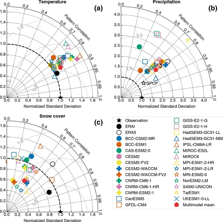
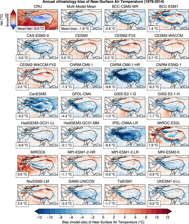
1070                                                       M. Lalande et al.: Climate change in the High Mountain Asia in CMIP6

Figure 3. Annual bias (model minus observation) computed over 1979–2014 for temperature, except the top left panel that shows the
climatology estimated from the CRU observation, used as the reference for the bias computation. The panel located at the right side of the
CRU observation shows the bias of the multimodel mean based on the 26 models shown in the figure. The black contour shows the political
frontiers and the bold black line the HMA domain located above 2500 m a.s.l., for which the spatial average of the bias is given in the bottom
left of each panel.

uct (grid cells with or without snow) might overestimate the             derestimation of snow cover (e.g., MPI-ESM1-2-HR, MPI-
snow cover in this often snowy area. The ESA CCI prod-                   ESM1-2-LR, NorESM2-LM). The annual overestimation of
uct shows a lower snow cover in general and in particular                the snow cover in most models arises mainly from a overly
in this region (not shown). It is therefore possible that in the         wide extension in the inner TP in winter (not shown). While
HK region the model biases actually reflect observation defi-            the excess of snow melts in summer in most of the mod-
ciencies, even if other factors affecting the model skill could          els, leading to a moderate bias during this season (Fig. 2),
be involved. The annual multimodel mean of snow cover is                 some models keep a persistent excess of snow even in sum-
overestimated by 12 % [−13 % to 43 %], corresponding to                  mer (e.g., HadGEM3-GC31-LL, HadGEM3-GC31-MM and
a relative bias of 52 % [−53 % to 183 %] over HMA com-                   IPSL-CM6A-LR), which partly explains the large dispersion
pared to NOAA CDR and can reach locally an absolute dif-                 between the models in terms of annual biases.
ference of 40 %, while a minority of models show a slight un-

Earth Syst. Dynam., 12, 1061–1098, 2021                                                     https://doi.org/10.5194/esd-12-1061-2021
M. Lalande et al.: Climate change in the High Mountain Asia in CMIP6                                                        1071

   All models show higher precipitation rates in comparison      higher number of models Fig. C1. These correlations would
with APHRODITE (Fig. B2), as seen in the annual cycles           likely be more positive if we used an observational refer-
(Fig. 2). Indeed, the multimodel annual mean bias of precip-     ence dataset that was not affected by snow undercatch is-
itation over HMA is 1.5 [0.3 to 2.9] mm d−1 , corresponding      sues. Nevertheless, the BCC-ESM1 and CAS-ESM2-0 mod-
to a relative bias of 143 % [31 % to 281 %]. The bias pat-       els show a strong correlation between snow cover and precip-
tern in terms of total precipitation is somehow proportional     itation biases (0.48 and 0.41, respectively). This link is par-
to the climatological pattern of precipitation, with stronger    ticularly striking for CAS-ESM2-0, for which the biases of
biases in the southeastern Himalayas, where high precipita-      snow cover and precipitation show similar patterns over the
tion rates are observed (Fig. B2). The quantification of the     TP and HM (Figs. B1 and B2), suggesting that snow cover
bias should be considered carefully for precipitation, because   biases in that case are partly due to an excess of precipitation.
the APHRODITE dataset strongly underestimates the pre-              The temperature and snow cover biases correlations with
cipitation rates at high elevations (Immerzeel et al., 2015).    the surface elevation show a more uniform behavior among
Anyway, the dry bias found in the southern flank of the Hi-      the models. In general, an anticorrelation between temper-
malayas, coupled with a positive bias of precipitation over      ature bias and elevation is found, whereas snow cover cor-
TP, suggests an overly coarse resolution to represent the oro-   relates positively with the elevation. The higher the eleva-
graphic barrier that blocks the northward moisture flux, a       tion, the greater the biases for temperature and snow cover,
limitation especially pronounced during the Asian summer         suggesting that the models have difficulty representing phys-
monsoon that induces strong precipitation rates in the south     ical processes at high elevation. The link between precipi-
of HMA.                                                          tation bias and elevation is less pronounced with fewer sig-
                                                                 nificant correlations (e.g., BCC-ESM1, CNRM-CM6-1-HR,
3.4   Spatial bias correlation
                                                                 HadGEM3-GC31-MM), which can either be positive or neg-
                                                                 ative.
To investigate the potential links between the biases of the        These spatial correlations are of course region and sea-
different variables, the correlation patterns between the bi-    son dependent. For example, we observe stronger correla-
ases of temperature, snow cover, precipitation and surface       tions between precipitation and snow cover biases in win-
elevation are shown in (Fig. 4). For most of the models, a       ter over TP, while the latter is stronger in summer over HK
significant negative correlation is found between the biases     for most of models (Figs. C2 and C3). This may be related
of temperature and snow cover, highlighting the influence of     to an excess of moisture supply over TP in winter, due to
these two variables on each other. However, it is not possible   the lack of orographic barrier effect because of the coarse
to deduce whether it is the snow cover bias that induces the     resolution of the models, resulting in too much snow accu-
temperature bias or the opposite. The strongest correlations     mulation, which is more likely to persist due to winter cold
between temperature and snow cover are found for the IPSL-       temperatures over the TP. Concerning the excess of summer
CM6A-LR and the MIROC-ES2L models, suggesting that               precipitation in HK, this may be due to an overextension of
these biases are exacerbated by feedbacks between these two      precipitation towards the west of the Himalayan mountain
variables, while lower correlations are found with precipita-    range during the monsoon period. However, this last correla-
tion biases. On the contrary, some models (e.g., HadGEM3-        tion, supporting the idea that the excess snow cover may be
GC31-MM) show a surprisingly positive correlation between        due to excess precipitation for some models, does not neces-
temperature and snow cover, suggesting that other processes      sarily explain the cold bias at the surface. For example, the
can play a role in the development of biases (aerosol deposi-    HadGEM3 models have strong significant correlations be-
tion on snow, cloud cover, tropospheric biases, etc.).           tween snow cover and precipitation biases over the TP (0.63
   The correlations between the biases of temperature and        and 0.66 annually) but do not show a significant surface cold
precipitation are generally weaker but with negative and         bias (−0.12 and −0.18 ◦ C; Fig. C3). The relationship of the
significant values between −0.12 and −0.37 (except for           biases with altitude is not always verified either, especially
CanESM5, which has a positive correlation of 0.16). This         for models showing warm biases such as the CESM2 family
seems counterintuitive as we generally expect precipitation      of models over the TP in summer.
rates to increase with temperature unless dynamical changes
of the atmosphere could induce an opposite signal at the re-     3.5   Metrics
gional scale. However, the positive precipitation model bi-
ases are likely due to the underestimation of solid precip-      Spatial RMSE and mean biases are computed over HMA for
itation in the APHRODITE observation, which would sug-           the 26 models (Fig. 5). CESM2, CESM2-WACCM and MPI-
gest an unrealistic excess of precipitation in the models.       ESM1-2-HR show the lowest temperature RMSE (∼ 2.5 ◦ C),
Therefore, these negative correlations are potentially not re-   with a mean bias smaller than 1 ◦ C, while worse performing
liable and have to be considered carefully. The comparison       models are CNRM-CM6-1, IPSL-CM6A-LR and CNRM-
with GPCP shows correlations between the biases of tem-          CM6-1-HR with RMSE exceeding 7 ◦ C. The best models for
perature and precipitation that reach positive values for a      temperature are not necessarily the best ones for snow cover

https://doi.org/10.5194/esd-12-1061-2021                                          Earth Syst. Dynam., 12, 1061–1098, 2021
1072 M. Lalande et al.: Climate change in the High Mountain Asia in CMIP6 Figure 4. Pattern correlations of the annual model biases. The first row shows the temperature bias normalized with the strongest temperature bias found among the 26 models (CNRM-CM6-1-HR). The following rows show the pattern correlations computed between temperature and snow cover biases (second row), temperature and precipitation biases (third row), snow cover and precipitation biases (fourth row). The fifth to the seventh rows show the correlation between biases and surface elevation estimated from GMTED2010 for temperature, snow cover and precipitation. All biases are annual and computed over 1979–2014. Bold characters highlight significant correlation (p value < 0.05). and precipitation (e.g., HadGEM3-GC31-LL, HadGEM3- MIROC-ES2l) to a maximum of 0.8 (GFDL-CM4). Overall, GC31-MM, UKESM1-0-LL). RMSE for snow cover ranges the spatial variance is higher for almost all the models as from about 10 % to 45 %, and most of the models show a compared to observations for both the temperature (the nor- positive snow cover bias over HMA. RMSE for precipita- malized standard deviation reaching 1.5 for the worst model) tion ranges from over 1 to 3.5 mm d−1 , while mean biases are and the precipitation (the normalized standard deviation ex- all positive, ranging from about 0.5 mm d−1 to slightly over ceeding 4 for the worst model). This is the contrary for snow 2 mm d−1 (Fig. 5c), as we already discussed in Sect. 3.3. cover, a variable for which the models show smaller spatial On the right panels of Fig. 5 (b, d, f), the RMSE and heterogeneities in comparison to the observational reference, mean bias are ranked by model resolution. Finer-resolution with a normalized standard deviation generally lower than models do not show better skill for temperature, snow cover 1, and varying between 0.4 and 1.4 for all the models. The and precipitation, suggesting that GCM resolution is not larger temperature standard deviation found for the models is the more important criterion for climate modeling over this partly explained by the general cold bias over HMA that en- region. This general assumption is not the case for all hances the temperature contrast between the high-elevation model families. For example, MPI-ESM1-2-LR (1.9◦ × 1.9◦ ) areas and the surrounding plains. The excess of precipitation and MPI-ESM1-2-HR (0.9◦ × 0.9◦ ) do show slight improve- found in the models over the area located under the influence ments for all variables with increasing resolution. However, of the Asian monsoons also explains the high standard de- for CNRM-CM6-1 (1.4◦ × 1.4◦ ) and its high-resolution ver- viation found in the models for this variable. In contrast, the sion CNRM-CM6-1-HR (0.5◦ × 0.5◦ ), the increase in reso- low standard deviation found in the model for the snow cover lution leads to a degradation for temperature and snow cover, is likely related to the overly extended and overly homoge- while there is a slight improvement for precipitation. neous snow cover over TP and its surrounding mountains, The Taylor diagram (Taylor, 2001) shown in Fig. 6 is used while the TP in observations is most often free of snow. An- to investigate the realism of the spatial variability simulated other interesting point is that both ERA-Interim and ERA5 in the models as compared to observational references. Over- do not perform much better than the CMIP6 models (except all, the models perform better for temperature than for pre- ERA-Interim for temperature and snow cover likely due to cipitation, whereas the model skill is even smaller for snow IMS snow cover assimilation over HMA), suggesting general cover. The pattern correlation (PCC) ranges from 0.7 to 0.9 weaknesses in the models used commonly for climate mod- for temperature, whereas it takes lower values for precipita- eling and for the production of atmospheric reanalysis, while tion varying from 0.6 to 0.8 for most of the models, except the multimodel mean has intermediate performance among for HadGEM3-GC31-MM, for which it reaches 0.9 and for the models. five other models showing a lower PCC below 0.6. For snow Overall, it is challenging to discard any model from this cover, the model PCC is even lower and also heterogeneous spatial analysis, as well as RMSE and bias metrics, because among the models, varying from negative values (−0.17 for of both a large heterogeneity of skill found among the mod- Earth Syst. Dynam., 12, 1061–1098, 2021 https://doi.org/10.5194/esd-12-1061-2021
M. Lalande et al.: Climate change in the High Mountain Asia in CMIP6 1073
Figure 5. Annual spatial RMSE and bias computed over HMA with respect to CRU, NOAA CDR and APHRODITE, respectively, for
temperature, snow cover and precipitation (a, c, e). Models are ranked by increasing RMSE for temperature and the multimodel mean
appears in the first histogram. The approximate original model’s resolution is given, but all metrics are computed on a common 1◦ × 1◦ grid
after interpolation. Panels (b, d, f) are similar to (a, c, e) with models ranked as a function of their original mean lat/long resolution. Blue
and red crosses correspond respectively to RMSE and mean bias.
els and a skill that varies also from one variable to another for until 50 % to climate trends computed over 50 years (Deser
the same model. This finding suggests that there is no reason et al., 2020). However, this contribution decreases when con-
to exclude some models for climate analysis purposes in this sidering areas closer to the tropics and when integrating cli-
area in particular when looking at future projections. Never- mate signals over large domains (Hawkins et al., 2016). The
theless, to explore this question deeper, the potential relation- climate trends in HMA are explored over the period 1979–
ship between biases and trends is investigated in Sect. 4.2. 2014 by comparing observational datasets and multimodel
mean computed with a single member for each model to
give the same weighting to each model (Fig. 7). This com-
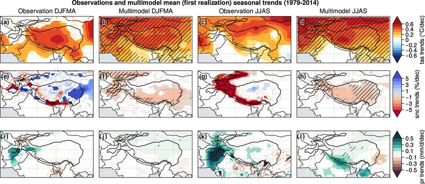
4 Historical trends analysis parison should be considered carefully, since observational
datasets reflect the superposition of both the internal variabil-
Disentangling the trends related to internal variability from ity and the forced signals whereas the internal variability is
the forced signals related to anthropogenic forcing is chal- partly filtered out when averaging the model outputs. How-
lenging. At midlatitudes, internal variability can contribute
https://doi.org/10.5194/esd-12-1061-2021 Earth Syst. Dynam., 12, 1061–1098, 2021You can also read