Comparison of CMIP6 historical climate simulations and future projected warming to an empirical model of global climate
←
→
Page content transcription
If your browser does not render page correctly, please read the page content below
Earth Syst. Dynam., 12, 545–579, 2021
https://doi.org/10.5194/esd-12-545-2021
© Author(s) 2021. This work is distributed under
the Creative Commons Attribution 4.0 License.

       Comparison of CMIP6 historical climate simulations and
            future projected warming to an empirical
                      model of global climate
         Laura A. McBride1 , Austin P. Hope2 , Timothy P. Canty2 , Brian F. Bennett2 , Walter R. Tribett2 , and
                                                Ross J. Salawitch1,2,3
       1 Department   of Chemistry and Biochemistry, University of Maryland College Park, College Park, 20740, USA
                                     2 Department of Atmospheric and Oceanic Science,

                              University of Maryland College Park, College Park, 20740, USA
                                       3 Earth System Science Interdisciplinary Center,

                              University of Maryland College Park, College Park, 20740, USA
                                Correspondence: Laura A. McBride (mcbridel@umd.edu)

                                 Received: 28 August 2020 – Discussion started: 8 September 2020
                            Revised: 30 March 2021 – Accepted: 1 April 2021 – Published: 10 May 2021

      Abstract. The sixth phase of the Coupled Model Intercomparison Project (CMIP6) is the latest modeling effort
      for general circulation models to simulate and project various aspects of climate change. Many of the general
      circulation models (GCMs) participating in CMIP6 provide archived output that can be used to calculate effec-
      tive climate sensitivity (ECS) and forecast future temperature change based on emissions scenarios from several
      Shared Socioeconomic Pathways (SSPs). Here we use our multiple linear regression energy balance model, the
      Empirical Model of Global Climate (EM-GC), to simulate and project changes in global mean surface temper-
      ature (GMST), calculate ECS, and compare to results from the CMIP6 multi-model ensemble. An important
      aspect of our study is a comprehensive analysis of uncertainties due to radiative forcing of climate from tro-
      pospheric aerosols (AER RF) in the EM-GC framework. We quantify the attributable anthropogenic warming
      rate (AAWR) from the climate record using the EM-GC and use AAWR as a metric to determine how well
      CMIP6 GCMs replicate human-driven global warming over the last 40 years. The CMIP6 multi-model ensem-
      ble indicates a median value of AAWR over 1975–2014 of 0.221 ◦ C per decade (range of 0.151 to 0.299 ◦ C
      per decade; all ranges given here are for 5th and 95th confidence intervals), which is notably faster warming
      than our median estimate for AAWR of 0.157 ◦ C per decade (range of 0.120 to 0.195 ◦ C per decade) inferred
      from the analysis of the Hadley Centre Climatic Research Unit version 5 data record for GMST. Estimates of
      ECS found using the EM-GC assuming that climate feedback does not vary over time (best estimate 2.33 ◦ C;
      range of 1.40 to 3.57 ◦ C) are generally consistent with the range of ECS of 1.5 to 4.5 ◦ C given by the IPCC’s
      Fifth Assessment Report. The CMIP6 multi-model ensemble exhibits considerably larger values of ECS (median
      3.74 ◦ C; range of 2.19 to 5.65 ◦ C). Our best estimate of ECS increases to 3.08 ◦ C (range of 2.23 to 5.53 ◦ C) if
      we allow climate feedback to vary over time. The dominant factor in the uncertainty for our empirical deter-
      minations of AAWR and ECS is imprecise knowledge of AER RF for the contemporary atmosphere, though
      the uncertainty due to time-dependent climate feedback is also important for estimates of ECS. We calculate the
      likelihood of achieving the Paris Agreement target (1.5 ◦ C) and upper limit (2.0 ◦ C) of global warming relative to
      pre-industrial for seven of the SSPs using both the EM-GC and the CMIP6 multi-model ensemble. In our model
      framework, SSP1-2.6 has a 53 % probability of limiting warming at or below the Paris target by the end of the
      century, and SSP4-3.4 has a 64 % probability of achieving the Paris upper limit. These estimates are based on
      the assumptions that climate feedback has been and will remain constant over time since the prior temperature
      record can be fit so well assuming constant climate feedback. In addition, we quantify the sensitivity of future
      warming to the curbing of the current rapid growth of atmospheric methane and show that major near-term limits

Published by Copernicus Publications on behalf of the European Geosciences Union.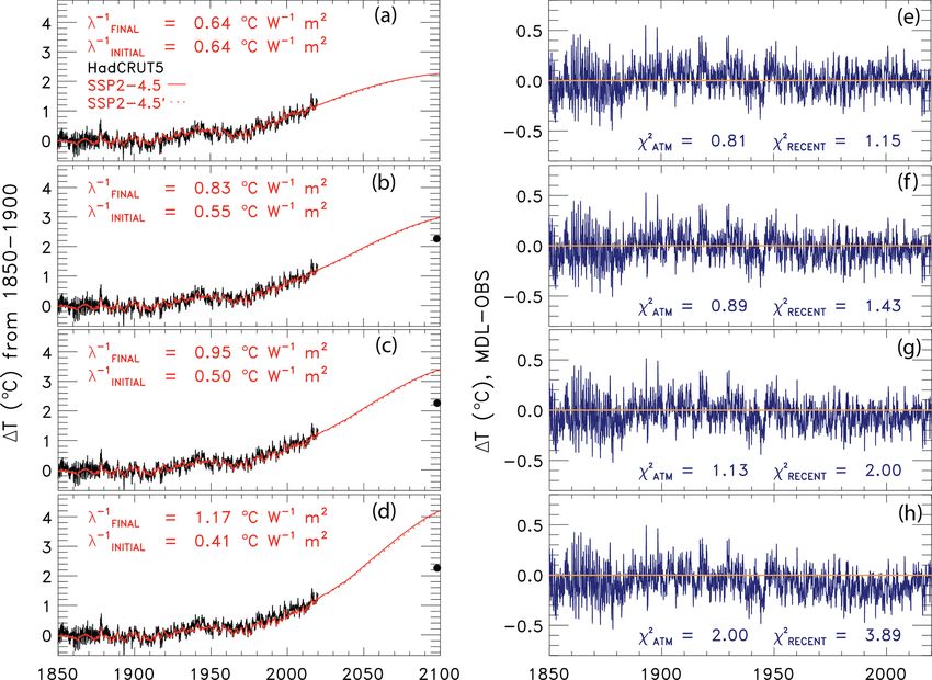
546                            L. A. McBride et al.: Comparison of CMIP6 warming to an empirical model of global climate

       on the future growth of methane are especially important for achievement of the 1.5 ◦ C goal of future warming.
       We also quantify warming scenarios assuming climate feedback will rise over time, a feature common among
       many CMIP6 GCMs; under this assumption, it becomes more difficult to achieve any specific warming target.
       Finally, we assess warming projections in terms of future anthropogenic emissions of atmospheric carbon. In our
       model framework, humans can emit only another 150 ± 79 Gt C after 2019 to have a 66 % likelihood of limiting
       warming to 1.5 ◦ C and another 400 ± 104 Gt C to have the same probability of limiting warming to 2.0 ◦ C. Given
       the estimated emission of 11.7 Gt C per year for 2019 due to combustion of fossil fuels and deforestation, our
       EM-GC simulations suggest that the 1.5 ◦ C warming target of the Paris Agreement will not be achieved unless
       carbon and methane emissions are severely curtailed in the next 10 years.

1   Introduction                                                  et al., 2017). Our anthropogenic components also include
                                                                  the effect of land-use change (i.e., deforestation) on Earth’s
The goals of the Paris Agreement, negotiated in Decem-            albedo and the export of heat from the atmosphere to the
ber of 2015, are to keep global warming below 2.0 ◦ C rel-        ocean as the atmosphere warms.
ative to the start of the Industrial Era and pursue efforts to       Our analysis builds on the work of Canty et al. (2013) and
limit global warming to 1.5 ◦ C. General circulation mod-         Hope et al. (2017) and includes several key updates. One
els (GCMs) project future temperature change using various        is the extension back in time of our analysis to 1850. The
evolutions of greenhouse gases and determine the likelihood       Hadley Centre Climatic Research Unit (Morice et al., 2012,
of achieving the goals of the agreement. Many GCMs are            2021), Berkeley Earth Group (Rohde and Hausfather, 2020),
participating in the sixth phase of the Coupled Model In-         and Cowtan and Way (2014) provide GMST records start-
tercomparison Project (CMIP6) to quantify how the models          ing in 1850, which now allows for simulations of GMST that
represent different aspects of climate change (Eyring et al.,     cover 170 years. The second update is the use of the Shared
2016). Accurate projections of future temperature are critical    Socioeconomic Pathways (SSPs) (O’Neill et al., 2017) as
for achieving the goals of the Paris Agreement. Chapter 11 of     our climate scenarios for greenhouse gas and aerosol abun-
the IPCC’s Fifth Assessment Report shows that some of the         dances. The third is the adoption of an upper ocean to our
previous generations of these models participating in phase       model, formulated in a manner that matches the equations
5 of the Coupled Model Intercomparison Project (CMIP5)            of Bony et al. (2006) and Schwartz (2012). A description of
(Taylor et al., 2012) tended to overestimate the increase in      the model, the various input parameters used, and the up-
global mean surface temperature (GMST) for the 21st cen-          dates listed above is given in Sect. 2. Section 3 shows results
tury (Kirtman et al., 2013). In this analysis we use a mul-       of CMIP6 and EM-GC comparisons to the historical climate
tiple linear regression energy balance model to quantify the      record, estimations of effective climate sensitivity (ECS) and
change in GMST from 1850–2019, project future changes in          comparisons of our model and CMIP6 projections of future
GMST, compare to the CMIP6 multi-model ensemble, and              GMST change. A discussion of these results is provided in
determine the likelihood of achieving the goals of the Paris      Sect. 4, along with concluding remarks.
Agreement.
   Several prior studies have used a multiple linear regression   2     Data and methodology
approach to model the GMST anomaly in order to quantify
the impact of anthropogenic and natural factors on climate        2.1    Empirical model of global climate
(Foster and Rahmstorf, 2011; Lean and Rind, 2008, 2009;           In this analysis we use the empirical model of global climate
Zhou and Tung, 2013). Typically, total solar irradiance, vol-     (EM-GC), which provides a multiple linear regression en-
canoes, and the El Niño–Southern Oscillation (ENSO) are           ergy balance simulation of GMST. As detailed in the follow-
the natural components represented in the multiple linear         ing paragraphs, the EM-GC solves for ocean heat uptake ef-
regression. Greenhouse gases and aerosols are the anthro-         ficiency (κ) and six regression coefficients to minimize the
pogenic factors. We use multiple linear regression, in con-       cost function in Eq. (1).
nection with a dynamic ocean module that accounts for the
export of heat from the atmosphere to the ocean, to repre-                          NMONTHS
                                                                                      X         1
sent the natural and anthropogenic components of the cli-         Cost function =              2
                                                                                                    (1TOBSi − 1TMDLi )2      (1)
                                                                                      i=1     σOBSi
mate system. In addition to the typical natural factors listed
above, we include the Atlantic Meridional Overturning Cir-        In this equation, 1TOBS represents a time series of observed
culation (AMOC), Pacific Decadal Oscillation (PDO), and           monthly GMST anomalies, 1TMDL is the modeled monthly
Indian Ocean Dipole (IOD) to provide a robust representa-         change in GMST, σOBS is the 1σ uncertainty associated with
tion of the natural climate system (Canty et al., 2013; Hope      each temperature observation, i is the index for each month,

Earth Syst. Dynam., 12, 545–579, 2021                                                https://doi.org/10.5194/esd-12-545-2021
L. A. McBride et al.: Comparison of CMIP6 warming to an empirical model of global climate                                    547

and NMONTHS is the total number of months used in the anal-     (Knight et al., 2005; Medhaug and Furevik, 2011; Stouffer
ysis. For this analysis, we trained the model from 1850–2019.   et al., 2006; Zhang and Delworth, 2007). We use the At-
The observed GMST anomalies are blended near-surface air        lantic multidecadal variability, based on the area-weighted
and sea surface temperature differences relative to the GMST    monthly mean sea surface temperature (SST) in the Atlantic
anomaly over 1850–1900, which is assumed to represent pre-      Ocean between the Equator and 60◦ N (Schlesinger and Ra-
industrial conditions.                                          mankutty, 1994), as a proxy for the strength of AMOC. A
   We consider several anthropogenic and natural factors        strong AMOC is characterized by northward flow of en-
to be components of 1TMDL . The radiative forcing (RF)          ergy that would otherwise be radiated to space, which occurs
due to greenhouse gases (GHGs), anthropogenic aerosols          in both the ocean and atmosphere and leads to particularly
(AER), land-use change (LUC), and the export of heat from       warm summers in Europe (Kavvada et al., 2013) as well as
the atmosphere to the world’s oceans are the anthropogenic      a number of other well-documented influences in other cli-
components of 1TMDL . The influence on GMST from to-            matic regions (Nigam et al., 2011). The total anthropogenic
tal solar irradiance (TSI), the El Niño–Southern Oscilla-       RF is used to detrend the AMOC signal. This method pro-
tion (ENSO), the Atlantic Meridional Overturning Circula-       vides a more realistic approach to infer the changes in the
tion (AMOC), volcanic eruptions that reach the stratosphere     strength of the AMOC and its effect on GMST than other
and enhance stratospheric aerosol optical depth (SAOD), the     detrending options (Canty et al., 2013).
Pacific Decadal Oscillation (PDO), and the Indian Ocean            The dimensionless parameter γ represents the sensitivity
Dipole (IOD) are the natural components of 1TMDL . Equa-        of the global climate to feedbacks that occur due to a change
tion (2) shows how we calculate 1TMDL , the modeled             in the RF of GHGs, AER, and LUC. We relate γ to the cli-
monthly change in GMST.                                         mate feedback parameter, λ6 , as shown in Eq. (3):
           1+ γ                                                               1
1TMDLi =        {GHG 1RFi + AER 1RFi + LUC 1RFi                 1+γ =                 ,                                     (3)
            λP                                                           1−       λ6
                                                                                  λP
 −QOCEAN i } + C0 + C1 × SAODi−6 + C2 × TSIi−1
 + C3 × ENSOi−2 + C4 × AMOCi + C5 × PDOi + C6                   where λ6 = 6 for all climate feedbacks, i.e., λ6 =
 × IODi                                                         λWater vapor +λLapse rate +λClouds +λSurface albedo . The relation
                                                                between λ6 and γ in Eq. (3) is commonly used in the cli-
                                                          (2)   mate modeling community (Sect. 8.6 of Solomon, 2007).
In Eq. (2), GHG 1RFi , AER 1RFi , and LUC 1RFi repre-           Our value of λ6 is related to the IPCC’s Fifth Assessment
sent monthly time series of the increase in the stratospheric   Report (Stocker et al., 2013; hereafter IPCC 2013) definition
adjusted values of the RF of climate (Solomon, 2007) since      of λ via λ6 = λP − λ.
1750. The parameter λP represents the response of a black          Our model explicitly accounts for the export of heat from
body to a perturbation in the absence of climate feedback       the atmosphere to the world’s oceans (i.e., ocean heat export
(3.2 W m−2 ; Bony et al., 2006). The SAOD, TSI, and ENSO        or OHE). The quantity QOCEAN in Eq. (2) represents OHE.
are lagged by 6, 1, and 2 months, respectively. The lag of      In our previous analyses (Canty et al., 2013; Hope et al.,
6 months for SAOD is representative of the time needed          2017), QOCEAN was subtracted outside the climate feedback
for the surface temperature to respond to a change in the       multiplicative term (1 + γ )/λP . We have rewritten Eq. (2) to
aerosol loading due to a volcanic eruption (Douglass and        be comparable to the formulation for this term used by Bony
Knox, 2005). This lag is the same as used by Lean and Rind      et al. (2006) and Schwartz (2012). Due to this update, our
(2008) and Foster and Rahmstorf (2011). The 1-month delay       model fits the historical climate record with higher values of
for TSI yields the maximum value of C2 , the solar irradi-      climate feedback, especially for strong aerosol cooling (see
ance regression coefficient. Lean and Rind (2008) and Fos-      Fig. S1 and the Supplement for more information). We calcu-
ter and Rahmstorf (2011) also use a 1-month lag for TSI in      late QOCEAN by simulating the long-term trend in observed
their analyses. The 2-month delay for the response of GMST      ocean heat content (OHC) as shown in Eqs. (4) and (5).
to ENSO is the lag needed to obtain the largest value of
the correlation coefficient of the Multivariate ENSO index      QOCEAN i = κ 1TATM,HUMAN i − 1TOCEAN,HUMAN i (4)
version 2 (MEI.v2) (Wolter and Timlin, 1993; Zhang et al.,                             OHE × 1t
                                                                κ=R           h                                               (5)
2019) versus the value of TENSO calculated by Thompson et               tEND     1+γ
                                                                       tSTART     λP {GHG RFi−72 + AER RFi−72
al. (2009). In Thompson et al. (2009), TENSO is the simu-
                                                                       +LUC RFi−72 } − [f0 i−72
                                                                                             P
lated response of GMST to variability induced by ENSO,                                           0   Q OCEAN   ]   dt
taking into consideration the effective heat capacity of the
atmospheric–ocean mixed layer. Lean and Rind (2008) used        The κ term is the ocean heat uptake efficiency (W m−2 ◦ C−1 )
a 4-month lag for ENSO.                                         and is based on the definition used in Raper et al. (2002),
   The term AMOCi represents the influence of the change        where κ is the ratio between the atmosphere and ocean
in the strength of the thermohaline circulation on GMST         temperature difference that best fits observed OHC data

https://doi.org/10.5194/esd-12-545-2021                                                 Earth Syst. Dynam., 12, 545–579, 2021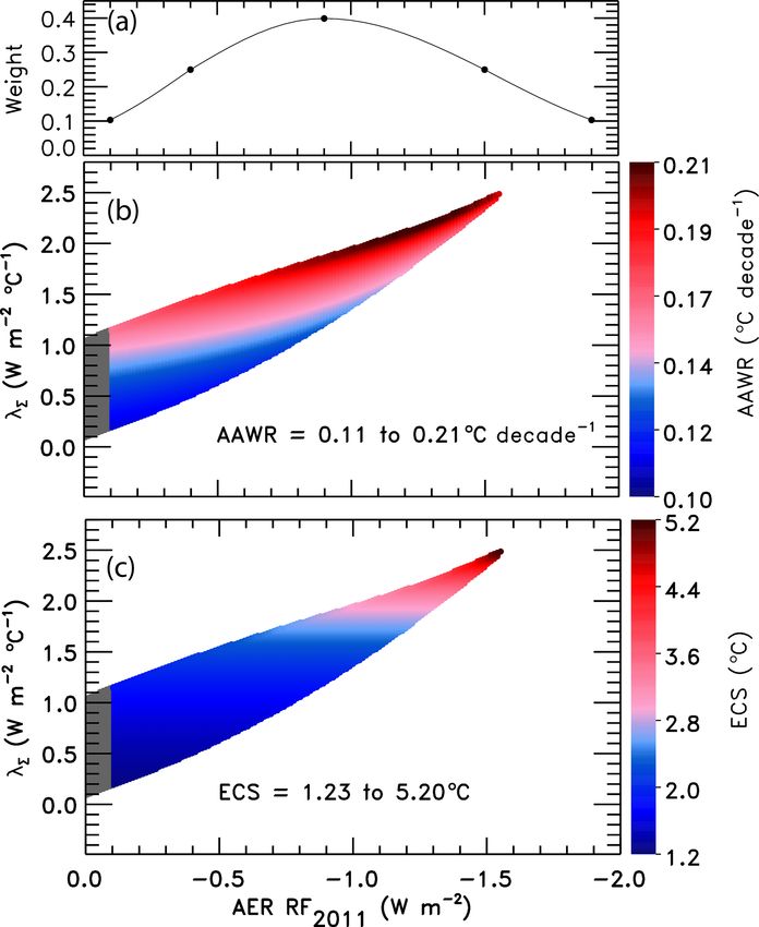
548                             L. A. McBride et al.: Comparison of CMIP6 warming to an empirical model of global climate

(Sect. 2.2.8 describes the OHC data records used in our anal-
ysis). The value of κ is determined based on the best fit
(described below) between QOCEAN and the observed OHC
record. The term 1TOCEAN,HUMAN represents the tempera-
ture response of the well-mixed top 100 m of the ocean due to
the total anthropogenically driven rise in OHC. This formula-
tion of 1TOCEAN,HUMAN allows the model ocean to warm in
response to an atmospheric warming. We use a 6-year lag (72
months) for QOCEAN to account for the time needed for the
energy leaving the atmosphere to heat the upper ocean and
penetrate to depth based on Schwartz (2012). Our analysis
of modeled GMST is insensitive to whether this 6-year lag
or the 10-year lag from Lean and Rind (2009) is used. The
tSTART and tEND limits on the integral in Eq. (5) are the start
and end years associated with each OHC record. The start
and end years vary between the five OHC records (see the
Supplement for the different start and end years). The con-
stant f0 term in Eq. (5) is a combination of the heat capacity
of ocean water, the fraction of total ocean volume in the sur-
face layer, and the fraction of total QOCEAN that warms the
surface layer; it is equal to 8.76 × 10⁻⁵ ◦ C m2 W−1 . We rep-
resent the global ocean as being 1 km deep for 10 % of the
ocean area (representing the continental shelves) and 4 km
deep for the remaining area, which approximates the average
depth of the actual world’s oceans to within 3 %: 3.7 km com-
pared to 3.682–3.814 km from Charette and Smith (2010).
Based on our analysis of decadal ocean warming as a func-
tion of depth extracted from CMIP5 GCMs, we have deter-
mined that 13.7 % of the rise in total OHC occurs in the well-
mixed upper 100 m of the ocean, the term represented by
1TOCEAN,HUMAN in Eq. (4). The bottom panel in Fig. 1 com-
pares our modeled OHC to the observed OHC record based
on the average of five data sets; the value of κ resulting in the
best simulation of observed OHC is shown.
   We use the reduced chi-squared (χ 2 ) metric to define the
goodness of fit between the modeled and measured GMST
anomaly for the atmosphere and also between simulated and           Figure 1. Measured and modeled GMST anomaly (1T ) relative to
observed OHC. Equations (6) and (7) show the calculations           a pre-industrial (1850–1900) baseline. (a) Observed (black) Had-
for χ 2 for the atmosphere, and Eq. (8) shows the calculation       CRUT5 and modeled (red) 1T from 1850–2019. This panel also
                                                                    displays the values of λ6 and χATM2    (see text) for this best-fit simu-
for χ 2 for the ocean. Minimization of the difference between
                                                                    lation. (b) Contributions from total human activity. This panel also
the measured and modeled GMST anomaly results in the
                                                                    denotes the best-estimate value of the attributable anthropogenic
EM-GC being able to replicate the observed rise in temper-          warming rate from 1975–2014 (black dashed) and the 2σ uncer-
ature over the past 170 years quite well, as shown in Fig. 1.       tainty in the slope for a model run that uses the best estimate of AER
We have added two additional new features to the model to           RF2011 of −0.9 W m−2 . (c) TSI (purple) and SAOD (light blue).
ensure accurate representation of the rise in OHC and the           (d) Influences from ENSO on 1T . (e) Contributions from AMOC
rise in GMST since 1940. The first new feature, Eq. (7), was        to 1T and to observed warming from 1975–2014. (f) Influences
added to ensure all simulations matched the past 80 years           from PDO (blue) and IOD (pink) on 1T . (g) Measured (black) and
                                       2
of observations well. Without the χRECENT      constraint, some     modeled (red) ocean heat content (OHC) as a function of time for
                              2                                                                                              2
                                                                    the average of five data sets (see text), the value of χOCEAN     for this
solutions with a value of χATM less than or equal to 2 have
visually poor simulations of the rise in GMST over the past         run, and the ocean heat uptake efficiency, κ, needed to provide the
                                                                    best fit to the OHC record. The error bars (blue) denote the uncer-
4 to 5 decades. The second new feature, Eq. (8), was added
                                                                    tainty in OHC used in this analysis (see Sect. 2.2.8).
because in the original model formulation some selections
of the radiative forcing due to tropospheric aerosols (AER
1RFi in Eq. 2) converged in a way that produced simulations
of OHC that seemed physically improper based on visual in-

Earth Syst. Dynam., 12, 545–579, 2021                                                     https://doi.org/10.5194/esd-12-545-2021
L. A. McBride et al.: Comparison of CMIP6 warming to an empirical model of global climate                                              549

spection of observed and modeled OHC. As a result of these                                             2
                                                                              The calculation of χRECENT       shown in Eq. (7) is used
two issues, all calculations shown here are subject to three               to constrain the model to match the observed changes in
goodness-of-fit constraints described by Eqs. (6) to (8).                  GMST over the time frame 1940–2019, a total of 80 years
                                                                           (NYEARS,REC equals 80). This time frame was chosen to in-
 2                       1                                                 clude a full cycle of AMOC, as the strength of the thermo-
χATM =
          NYEARS − NFITTING PARAMETERS − 1                                 haline circulation tends to vary on a period of 60–80 years
          NYEARS                                                           (Chen and Tung, 2018; Kushnir, 1994; Schlesinger and Ra-
           X                1
      ×                            (h1TOBSj i − h1TMDLj i)2          (6)   mankutty, 1994). As noted above, the χRECENT  2        constraint
              j =1
                      hσOBSj i2
                                                                           was added to our model framework because without this con-
 2                                          1                              straint the model is able to provide numerically good but poor
χRECENT =
                NYEARS,REC − NFITTING PARAMETERS − 1                       visual fits to the GMST anomaly under certain conditions
               NYEARS,                                                     (i.e., the red line in the top panel of Fig. 1 starts to strongly
                  X REC            1
          ×                               (h1TOBSj i − h1TMDLj i)2         deviate from the black line beginning in about 2000 under
                     j =1
                                hσOBSj i2                                  certain conditions). All model simulations shown below have
                                                                             2
                                                                           χRECENT     ≤ 2, representing a good fit to the observed rise
                                                                     (7)
                                        1                                  in GMST over the past 80 years, which results in modeled
χOCEAN2 =                                                                  GMST that replicates observed GMST for the entire time se-
                NYEARS − NFITTING PARAMETERS − 1
    NYEARS,OHC
                                                                           ries.
       X                1                                                     Figure 1 shows the observed (HadCRUT5) and mod-
×                                (hOHCOBSj i − hOHCMDLj i)2          (8)
       j =1
                     hσOBSj i2                                             eled GMST anomaly from 1850–2019 and the various an-
                                                                           thropogenic and natural components that constitute mod-
Here, , , and  in Eqs. (6)                          eled GMST. Figure 1a shows the value of climate feed-
and (7) represent the annually averaged observed GMST                      back, 1.62 W m−2 ◦ C−1 , that is needed to achieve a best fit to
anomaly, modeled GMST anomaly, and uncertainty                             the climate record for this simulation, resulting in values of
in the GMST anomaly, respectively. The variable                              2
                                                                           χATM                  2
                                                                                   = 0.80 and χOCEAN     = 0.31. Figure 1b is the total con-
NFITTING PARAMETERS is equal to 9 for typical simula-                      tribution of human activity to variations in GMST, which in-
tions, the sum of 7 (the number of regression coefficients)                cludes GHGs, AER, LUC, and the export of heat from the at-
plus 2 (model output parameters γ and κ). In Eq. (8),                      mosphere to the ocean. For the simulation shown, the aerosol
 and  represent the annual aver-                         radiative forcing is −0.9 W m−2 , the best estimate given by
aged observed and modeled OHC. The σOBS term in Eq. (8)                    IPCC 2013 (Myhre et al., 2013). This panel also notes the
is the uncertainty in the OHC record (see Sect. 2.2.8 for                  best estimate of the time rate of change in GMST attributed to
more information). The equation for all three formulations                 humans from 1975–2014, or the attributable anthropogenic
of χ 2 is based on annual averages rather than monthly time                warming rate (AAWR; see Sect. 2.3). Figure 1c illustrates the
series. We calculate χ 2 with annual values because the                    contribution to the GMST anomaly from TSI and SAOD over
autocorrelation functions of 1TOBS and 1TMDL display                       the 170-year period. The influences of ENSO and AMOC are
similar shapes using annual averages and do not match                      indicated in Fig. 1d and e, respectively. Furthermore, the con-
utilizing monthly averages (see the Supplement of Canty                    tribution of AMOC to the rise in GMST over 1975–2014 (the
et al., 2013, for a further explanation). The Hadley Centre                same time period used to define AAWR) is also specified in
Climate Research Unit (HadCRUT) version 4 uncertainties                    Fig. 1e (dotted black line). Figure 1f indicates the small effect
for GMST are used for the σOBS in Eqs. (6) to (8) for all of               of IOD and PDO on GMST in our model framework. The
the GMST records analyzed here (see Sect. 2.2.1 and the                    last panel, Fig. 1g, shows the time series of observed OHC
Supplement for more information). For Eqs. (6) to (8), we                  based on the average of five data sets for the upper 700 m of
define an acceptable fit to the climate record as χ 2 ≤ 2. The             the ocean (black points and blue error bars; see Sect. 2.2.8)
number of years (NYEARS ) varies across the three equations.               and the modeled value of OHC (red line). For this simula-
Equation (6) uses the total number of years in the GMST                    tion, a value of κ equal to 1.17 W m−2 ◦ C−1 fits the OHC
record, which for HadCRUT5 is 170 years. The number                        data best. This value of κ falls within the range of empiri-
of years in Eq. (8), NYEARS,OHC , depends on the OHC                       cal estimates for this parameter given by Raper et al. (2002).
data set used, as each data set spans a different range. The               The sum of the contributions of human activity, TSI, SAOD,
average of five OHC data sets, which we use as our primary                 ENSO, AMOC, PDO, and IOD to the GMST anomaly shown
OHC series, extends from 1955–2017, a total of 63 years.                   in Fig. 1b to f plus the value of C0 equals the modeled GMST
                 2
The value of χOCEAN      found using Eq. (8) is displayed in               anomaly, shown by the red line in Fig. 1a.
the bottom panel of Fig. 1. All model simulations shown                       Altering the training period of our model has a slight effect
                              2
throughout this paper have χOCEAN    ≤ 2, representing a good              on our results (see Figs. S2, S3, and the Supplement for in-
fit to the observed rise in OHC over the time of the data                  formation on various training periods). We project relatively
record.                                                                    similar results for end-of-century warming for training pe-

https://doi.org/10.5194/esd-12-545-2021                                                        Earth Syst. Dynam., 12, 545–579, 2021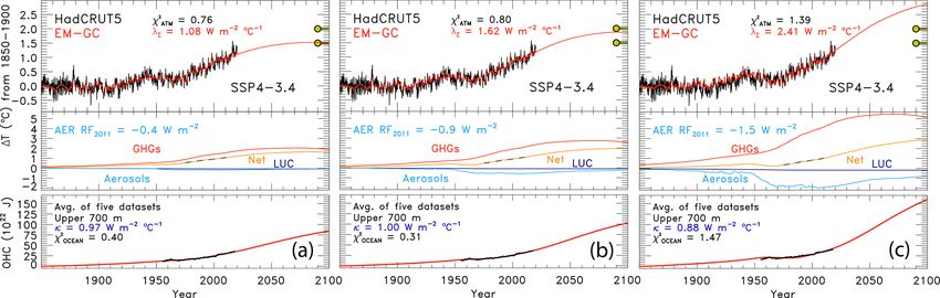
550 L. A. McBride et al.: Comparison of CMIP6 warming to an empirical model of global climate
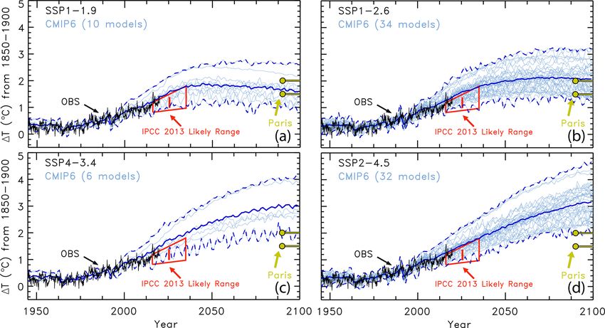
riods that start in 1850 and end in either 2009 or 1999 com- As part of CMIP6, the ScenarioMIP experiment (O’Neill
pared to results shown throughout the paper for a training pe- et al., 2016) includes eight SSPs (SSP1-1.9, SSP1-2.6, SSP4-
riod of 1850 to 2019, indicating the stability of our approach. 3.4, SSP2-4.5, SSP4-6.0, SSP3-7.0, SSP5-8.5, and SSP5-3.4-
As detailed in the Supplement, we do find some differences OS) that GCMs use to project future GMST. The first num-
from the results shown in the paper upon use of a training ber is the reference pathway that the scenario follows (i.e.,
period of 1850 to 1989 due to the reduction in the number of SSP1 follows the first SSP narrative), and the numbers after
years considered from the available OHC records. the dash are the target radiative forcing at the end of the cen-
tury (i.e., SSP1-2.6 reaches around 2.6 W m−2 in 2100). The
ScenarioMIP experiment designates Tier 1 and Tier 2 scenar-
2.2 Model inputs
ios. The Tier 1 scenarios are SSP1-2.6, SSP2-4.5, SSP3-7.0,
2.2.1 Temperature data and SSP5-8.5, and the Tier 2 scenarios are SSP1-1.9, SSP4-
3.4, SSP4-6.0, and SSP5-3.4-OS (an overshoot pathway that
We use seven global mean surface temperature anomaly follows SSP5-8.5 until around 2040, whereby carbon dioxide
records. These records include the Hadley Centre Climatic emissions drastically decrease and become negative in 2065).
Research Unit version 4 (HadCRUT4; Morice et al., 2012) Our analysis includes seven of the eight ScenarioMIP SSPs:
and version 5 (HadCRUT5; Morice et al., 2021) from all but the overshoot pathway. We highlight four in the main
1850–2019, National Centers for Environmental Informa- paper: two Tier 1 (SSP1-2.6 and SSP2-4.5) and two Tier 2
tion NOAAGlobalTemp v5 (NOAAGT; Smith et al., 2008; (SSP1-1.9 and SSP4-3.4) scenarios. An analysis of the other
Zhang et al., 2019) from 1880–2019, NASA Goddard In- three SSPs is included in the Supplement. Figure 2 shows
stitute of Space Studies Surface Temperature Analysis v4 the atmospheric abundance of the three major anthropogenic
(GISTEMP; Hansen et al., 2010) from 1880–2019, Berke- GHGs (carbon dioxide, methane, and nitrous oxide) for each
ley Earth Group (BEG; Rohde and Hausfather, 2020) from of the seven SSPs we consider and observations of the global
1850–2019, Cowtan and Way (2014) (CW14) from 1850– mean atmospheric abundance for these gases to the end of
2019, and the Japanese Meteorological Agency (JMA; Ishi- 2019 (Dlugokencky, 2020; Dlugokencky and Tans, 2020).
hara, 2006) from 1891–2019. We use the uncertainty time
series from HadCRUT4 for all GMST records because the
2.2.3 Greenhouse gases
HadCRUT4 uncertainty provides a realistic description of the
variation in GMST among the seven records (see the Supple- The historical values of GHG mixing ratios were provided
ment, Figs. S4 and S5, and Table S1 for more information). by Meinshausen et al. (2017b) from 1850–2014. We used
Our analysis primarily uses the HadCRUT5 GMST data set, the equations from Myhre (1998) to calculate the change in
but in some sections, results are shown for the other data sets. RF due to carbon dioxide (CO2 ), methane (CH4 ), nitrous ox-
All temperature anomalies are with respect to a pre-industrial ide (N2 O), ozone-depleting substances (ODSs), hydrofluoro-
baseline (1850–1900). To alter each data record so that the carbons, perfluorocarbons, and sulfur hexafluoride relative to
temperature anomaly is relative to the same pre-industrial RF in the year 1850. We also used the updated pre-industrial
baseline, we adjust all data sets relative to the HadCRUT5 values of CH4 and N2 O from IPCC 2013 and the radiative
baseline of 1961–1990. We then adjust each data set by the efficiencies from the WMO (2018). The radiative forcing of
same amount to the HadCRUT5 pre-industrial baseline as de- CH4 also includes the 15 % enhancement from the increase
scribed in the Supplement. in stratospheric water vapor due to rising atmospheric CH4
(Myhre et al., 2007). Values of GHG mixing ratios, other than
2.2.2 Shared Socioeconomic Pathways ODSs, from 2015–2100 are from the SSP database (Calvin et
al., 2017; Fricko et al., 2017; Fujimori et al., 2017; Kriegler
For this analysis, we use the estimates of the future abun- et al., 2017; Rogelj et al., 2018; van Vuuren et al., 2017) and
dances of greenhouse gases and aerosols provided by the are provided on a decadal basis. These mixing ratios were in-
SSPs. There are 26 scenarios, five baseline pathways, and terpolated onto a monthly timescale. We used the estimates
21 mitigation scenarios. The baseline pathways follow spe- of future ODS abundances provided in Table 6-4 of the 2018
cific narratives for factors such as population, education, eco- Ozone Assessment Report (Carpenter et al., 2018) because
nomic growth, and technological developments of sources of the SSP database did not provide these estimates. We also in-
renewable energy (Calvin et al., 2017; Fricko et al., 2017; clude tropospheric ozone (OTROP3 ) as a GHG because tropo-
Fujimori et al., 2017; Kriegler et al., 2017; van Vuuren et al., spheric ozone rivals N2 O as the third most important anthro-
2017) to represent several possible futures encompassing dif- pogenic GHG (Fig. 8.15 of Myhre et al., 2013). The RF due
ferent challenges for adaptation to and mitigation of climate to OTROP
3 from the Representative Concentration Pathways
change as illustrated in Fig. 1 of O’Neill et al. (2014). The 21 (RCPs) provided by the Potsdam Institute for Climate Im-
mitigation scenarios follow one of the baseline pathways but pact Research (Meinshausen et al., 2011) is used because the
include specific climate policy to reach a designated radiative SSP database does not provide estimates. Values of RF due to
forcing at the end of the century. OTROP
3 from RCP2.6, RCP4.5, RCP6.0, and RCP8.5 are sub-
Earth Syst. Dynam., 12, 545–579, 2021 https://doi.org/10.5194/esd-12-545-2021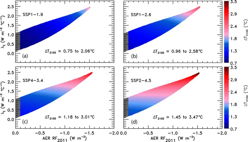
L. A. McBride et al.: Comparison of CMIP6 warming to an empirical model of global climate                                         551

Figure 2. Observed and projected greenhouse gas mixing ratios. (a) Carbon dioxide abundances from observations (black) and seven of the
ScenarioMIP SSPs (colors, as indicated). (b) Methane abundances from observations and ScenarioMIP SSPs. (c) Nitrous oxide abundances
from observations and ScenarioMIP SSPs.

stituted in for SSP1-2.6, SSP2-4.5, SSP4-6.0, and SSP5-8.5,           value of climate feedback (λ6 = 1.08 W m−2 ◦ C−1 ) needed
respectively. We created new time series for the RF due to            to fit the observed GMST record (Fig. 3a). The use of any of
OTROP
  3     for SSP4-3.4 and SSP3-7.0 using linear combinations           the values of AER RF2011 in Fig. 3 can result in a very good
of RF time series from RCP2.6 and RCP8.5, with weights                                                  2
                                                                      fit to the climate record (i.e., χATM        2
                                                                                                            ≤ 2, χRECENT    ≤ 2, and
based on the end-of-century total RF value due to all GHGs              2
                                                                      χOCEAN ≤ 2).
of the respective time series. Finally, the RF time series for           We use the total aerosol RF time series provided by the
OTROP
  3     from RCP2.6 was also used for SSP1-1.9. Figure S6             SSP database for each SSP scenario. The database provides
shows the ozone RF time series used in this analysis, and the         AER RF from 2005–2100, with values for all SSPs nearly
Supplement provides more information about the creation of            identical until about 2010 (Riahi et al., 2017; Rogelj et al.,
the time series for the RF due to OTROP
                                   3     .                            2018). In the EM-GC, we calculate temperature projections
                                                                      over the entire observational period beginning in 1850. We
                                                                      create AER RF time series that begin in 1850 and span the
2.2.4   Aerosol radiative forcing
                                                                      range of uncertainty given by Chapter 8 of IPCC 2013. We
The value of the change in total aerosol radiative forcing            use historical estimates of AER RF from 1850–2014 for the
(direct and indirect) in 2011 relative to pre-industrial (AER         four RCPs provided by the Potsdam Institute for Climate Re-
RF2011 ) is highly uncertain. Chapter 8 of the IPCC 2013 re-          search (Meinshausen et al., 2011). The AER RF value in
port gives a best estimate of AER RF2011 as −0.9 W m−2 ,              2014 from the appropriate historical estimate (i.e., RCP4.5
a likely range between −0.4 and −1.5 W m−2 , and a 5th                is used for SSP2-4.5) is scaled by a constant factor such
to 95th percent confidence interval between −0.1 and                  that the historical RCP value at the end of 2014 matches
−1.9 W m−2 (Myhre et al., 2013). This substantial range in            the SSP time series at the start of 2015. This scaling yields
AER RF2011 results in a large spread in future projections            a continuous time series for the RF of climate due to tro-
of global GMST. Figure 3 shows the effect of varying the              pospheric aerosols. This scaled time series has AER RF2011
value of AER RF2011 on projections of GMST in our EM-                 nearly equal to −1.0 W m−2 , which we take as the SSP-based
GC framework for the same SSP4-3.4 GHG scenario. The                  best estimate of the change in total aerosol radiative forcing
middle box in Fig. 3a, b, and c shows the contribution to             in 2011 relative to pre-industrial. Next, the single continu-
GMST of GHGs, LUC, AER, and net human activities. As                  ous time series is scaled, again by a constant multiplicative
the value of AER RF2011 decreases and aerosols cool more              factor, to match the IPCC 2013 best estimate and range of
strongly, the value of climate feedback (model parameter              uncertainty for AER RF2011 (Myhre et al., 2013). This pro-
λ6 ) rises, and the net contribution of the human impact on           cedure results in five additional time series of AER RF. Six
GMST by the end of the century increases. Depending on                time series of AER RF are created for each SSP, having val-
which value of AER RF2011 is used, the rise in GMST by                ues of AER RF2011 equal to −0.1, −0.4, −0.9, −1.0, −1.5,
the year 2100 for the SSP4-3.4 pathway could range from               and −1.9 W m−2 . Figure S7 shows these six AER RF time
1.5 ◦ C (Fig. 3a) to 2.8 ◦ C (Fig. 3c) relative to pre-industrial.    series for SSP1-2.6 and SSP4-3.4. In the EM-GC framework,
Strong aerosol cooling offsets a substantial fraction of GHG-         we further scale these six time series to create a total of 400
induced warming, and a large value of climate feedback                AER RF time series to fully analyze the range of AER RF2011
(λ6 = 2.41 W m−2 ◦ C−1 ) is needed to fit the historical cli-         given by Myhre et al. (2013).
mate record (Fig. 3c). In this case, future warming is large,
well above the goals of the Paris Agreement, by the end of
the century. Conversely, weak aerosol cooling offsets only a
small fraction of GHG-induced warming, resulting in a small

https://doi.org/10.5194/esd-12-545-2021                                                   Earth Syst. Dynam., 12, 545–579, 2021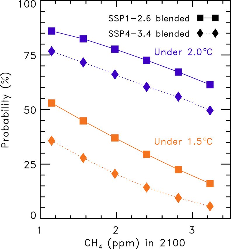
552                               L. A. McBride et al.: Comparison of CMIP6 warming to an empirical model of global climate

Figure 3. Measured (HadCRUT5) and EM-GC simulated GMST anomaly (1T ) relative to a pre-industrial (1850–1900) baseline, as well as
projected 1T to the end of the century for SSP4-3.4. The top box in each panel displays observed (black) and simulated (red) 1T , as well as
                        2
the values of λ6 and χATM     for each model run. The Paris Agreement target (1.5 ◦ C) and upper limit (2.0 ◦ C) are shown (gold circles). The
middle boxes show the contribution of GHGs, aerosols, and land-use change to 1T , as well as the net human component. The bottom boxes
compare observed (black) and modeled (red) values of OHC for simulations constrained by the average of five data sets (see text) and also
                                                                                                                  2
provides the numerical values of κ needed to obtain best fits to the OHC record as well as best-fit values of χOCEAN     . The only difference
between (a), (b), and (c) is the time series for RF due to tropospheric aerosols used to constrain the EM-GC; values of AER RF2011 for each
time series are (a) −0.4 W m−2 , (b) −0.9 W m−2 , and (c) −1.5 W m−2 .

2.2.5   Total solar irradiance and stratospheric aerosol                 append the SAOD after 2018, we took the average difference
        optical depth                                                    between the two time series for the overlapping months and
                                                                         then adjusted the CALIPSO time series by this offset. This
We use the TSI time series provided for the CMIP6 models                 slight adjustment to the CALIPSO record has no bearing on
from 1850–2014 (Matthes et al., 2017) and append values                  our results, since the effect of volcanic activity on GMST has
from the Solar Radiation and Climate Experiment (SORCE)                  been small over the past 2 decades (Fig. 1c). We set the term
(Dudok de Wit et al., 2017) for 2015 to the end of 2019.                 SAODi in Eq. (2) equal to the value in December 2019 from
The values of TSIi used in Eq. (2) are differences of monthly            the start of 2020 until 2100.
mean values minus the long-term average (i.e., TSI anoma-
lies). Consistent with prior studies (e.g., Lean and Rind,
2008; and Foster and Rahmstorf, 2011), variations in solar               2.2.6    El Niño–Southern Oscillation, Pacific Decadal
irradiance due to the 11-year solar cycle have a small but                        Oscillation, and Indian Ocean Dipole
noticeable effect on the EM-GC simulation of the GMST
anomaly (Fig. 1c). For projections of future warming, we set             We use the MEI.v2 (Wolter and Timlin, 1993; Zhang et al.,
the term TSIi in Eq. (2) equal to zero from the start of 2020            2019) to characterize the influence of ENSO on GMST. In
until 2100.                                                              order to obtain a time series that spans the entire training pe-
   The time series for SAOD is a combination of values com-              riod of our model, 1850–2019, we append three time series
puted from extinction coefficients for the CMIP6 GCMs (Ar-               to create an MEI.v2 over the full extent of our model training
feuille et al., 2014) from 1850–1978 and the Global Space-               period. The MEI.v2 provides 2-month averages of empiri-
based Stratospheric Aerosol Climatology (GloSSAC v2.0)                   cal orthogonal functions of five different climatic variables
(Thomason et al., 2018) from 1979–2018. Extinction coef-                 from 1979 to the present (Zhang et al., 2019). To have the
ficients at 550 nm were integrated from the tropopause to                ENSO index extend back to 1850, we compute differences
39.5 km and averaged over the globe using a cosine of lat-               in SST anomalies over the tropical Pacific basin as defined
itude weighting. The CMIP6 and GloSSAC extinction coef-                  by the MEI.v2 from 1850–1870 using HadSST3 (Kennedy
ficients span 80◦ S to 80◦ N. To extend the SAOD time series             et al., 2011). Our internal computation of this surrogate for
to the end of 2019, we use the level 3 gridded SAOD product              the MEI is then appended to the MEI.ext of Wolter and Tim-
from the Cloud–Aerosol Lidar and Infrared Pathfinder Satel-              lin (2011), which extends from 1871–1978, and the MEI.v2
lite Observations (CALIPSO) (Vaughan et al., 2004). Time                 of (Zhang et al., 2019) (1979–2019). This full time series
series of globally averaged SAOD from CALIPSO have a                     provides a representation of ENSO that covers 1850 to the
very similar shape as the GloSSAC time series over the pe-               present. Consistent with prior regression-based approaches
riod of overlap (2006–2018) with a slight offset because                 (Foster and Rahmstorf, 2011; Lean and Rind, 2008), we find
GloSSAC uses estimates of CALIPSO data for SAOD. To                      that a significant portion of the monthly and at times annual

Earth Syst. Dynam., 12, 545–579, 2021                                                         https://doi.org/10.5194/esd-12-545-2021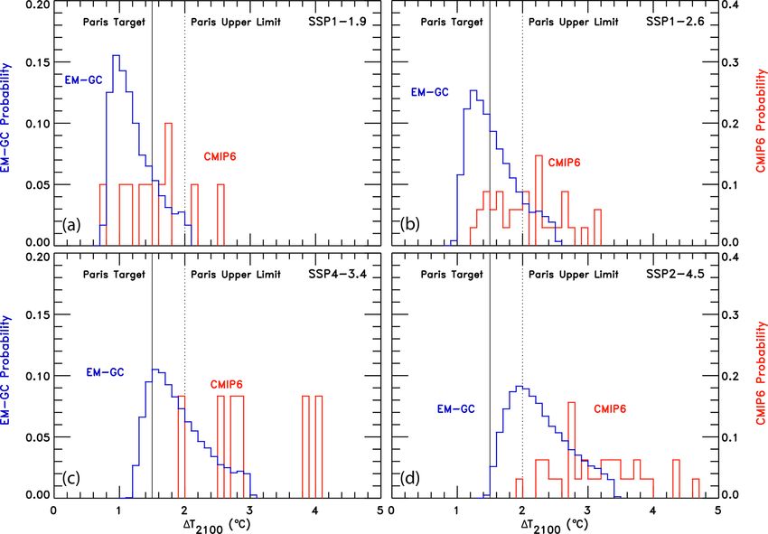
L. A. McBride et al.: Comparison of CMIP6 warming to an empirical model of global climate                                      553

variation in GMST is well explained by ENSO (Fig. 1d). As          amplitude component of the thermohaline circulation (Canty
for the other natural terms, we assume ENSOi in Eq. (2) is         et al., 2013). As noted above and shown in Fig. 1, a con-
zero for 2020–2100.                                                siderable portion of the long-term variability in GMST is at-
   The Pacific Decadal Oscillation is the leading principal        tributed to variations in the strength of the AMOC, including
component of North Pacific monthly SST variability pole-           about 0.025 ◦ C per decade over the 1975–2014 time period.
ward of 20◦ N (Barnett et al., 1999). The PDO index main-          There is considerable debate about the validity of the use of
tained by the University of Washington provides monthly            a proxy such as the AMV index as a surrogate for the cli-
values from 1900–2018. The PDO varies on a multidecadal            matic effects of the AMOC that is centered mainly around
timescale and affects climate in the North Pacific and North       how much of the variability of the index is either internal or
America, and it has secondary effects in the tropics (Bar-         externally forced (Haustein et al., 2019; Knight et al., 2005;
nett et al., 1999). In our model framework, the expression         Medhaug and Furevik, 2011; Stouffer et al., 2006). We stress,
of PDO on GMST is dependent on the model specification             as explained in Sect. 2.3, that none of our major scientific
of the AER RF time series, as shown in Fig. S8. At low val-        conclusions are altered if we neglect AMV as a regression
ues of AER RF2011 , such as −0.1 W m−2 , the effect of PDO         variable.
on GMST is negligible and the contribution from the AMOC
dominates. At high values of AER RF2011 (−1.5 W m−2 ), the         2.2.8   Ocean heat content records
effect of PDO on GMST is equal to the contribution from the
AMOC. At high values of AER RF2011 , we obtain results             Ocean heat content data records from five recent and inde-
similar to findings from England et al. (2014) and Trenberth       pendent papers are used in this study. We utilize OHC data
and Fasullo (2013) that show the PDO exhibits an apprecia-         from Balmaseda et al. (2013), Carton et al. (2018), Cheng
ble influence on GMST, especially for the 2000–2010 time           et al. (2017), Ishii et al. (2017), and Levitus et al. (2012), as
period.                                                            well as the average of the records to model the export of heat
   The Indian Ocean Dipole is based on the difference in           (OHE) from the atmosphere to the ocean. Figure S9 shows
the anomalous sea surface temperature (SST) between the            these five OHC records and the multi-measurement average.
western equatorial Indian Ocean (50–70◦ E and 10◦ S–10◦ N)         While most of these data sets have a common origin, they
and the southeastern equatorial Indian Ocean (90–110◦ E            differ in how extensive temporal and spatial gaps in the cov-
and 10◦ S–0◦ N) as defined in Saji et al. (1999). We use           erage of ocean temperatures have been handled, ranging from
1◦ × 1◦ SSTs from the Centennial in situ Observation-Based         data assimilation (Carton et al., 2018) to an iterative radius-
Estimate (COBE) (Ishii et al., 2005) to create an IOD index        of-influence mapping method (Cheng et al., 2017). The five
from 1850–2019. As noted above and shown in Fig. 1f, the           data sets are all set to zero in 1986, which is the midpoint
regression coefficients for PDO and IOD are quite small. We        of the multi-measurement time series, by applying an offset
find little influence of either PDO or IOD in the HadCRUT5         for visual comparison. Since OHE (units: W m−2 ) is based
time series of GMST, but these terms are retained for com-         on the slope of each OHC data set, this offset has no im-
pleteness. We assume PDOi and IODi in Eq. (2) are zero after       pact on the computation of OHE from OHC that is central
the start of 2019 and 2020, respectively.                          to our study. For the computation of OHE from OHC, we
                                                                   use a value of the surface area of the world’s oceans equal
2.2.7   Atlantic Meridional Overturning Circulation
                                                                   to 3.3 × 10¹⁴ m2 (Domingues et al., 2008). The OHC records
                                                                   we analyze are for the upper 700 m of the ocean. To calcu-
We use the Atlantic multidecadal variability (AMV) index           late the OHE for the whole ocean, we multiply the OHE by
as the area-weighted monthly mean SST from HadSST4                 1/0.7 to account for the fact that the upper 700 m of the ocean
(Kennedy et al., 2019) between the Equator and 60◦ N in the        holds 70 % of the heat (Sect. 5.2.2.1, Solomon, 2007). When
Atlantic Ocean (Schlesinger and Ramankutty, 1994) to char-         we subtract the amount of heat going into the ocean in Eq. (2)
acterize the influence of the AMOC on GMST. The AMV in-            (QOCEAN ), we also must account for the difference in surface
dex is detrended using the RF anomaly due to anthropogenic         area between the global atmosphere and the world’s oceans.
activity over the historical time frame of the analysis, as dis-   Since the QOCEAN term is computed for the surface area of
cussed in Sect. 3.2.3 of Canty et al. (2013), because this de-     the ocean but the forcing is applied to the whole atmosphere,
trending option removes the influence of long-term global          we multiply the QOCEAN term by the ratio of the surface area
warming on the AMV index. The detrended AMV index                  of the ocean to the surface area of the atmosphere, which is
serves as a proxy for variations in the strength of the AMOC       0.67.
(Knight et al., 2005; Medhaug and Furevik, 2011; Zhang and            As noted above, the calculation of χOCEAN  2        shown in
Delworth, 2007), which has particularly noticeable effects on      Eq. (8) is used to constrain our model representation of the
climate in the Northern Hemisphere (Jackson et al., 2015;          rise in OHC. Only model runs that provide a good fit to the
Kavvada et al., 2013; Nigam et al., 2011). For this analy-         observed OHC record are shown below. For these five OHC
sis, the index has been Fourier-filtered to remove frequencies     data sets, uncertainty estimates are not always provided. Fur-
above 1 / 9 per year to retain only the low-frequency, high-       thermore, some studies that do provide uncertainties give es-

https://doi.org/10.5194/esd-12-545-2021                                                Earth Syst. Dynam., 12, 545–579, 2021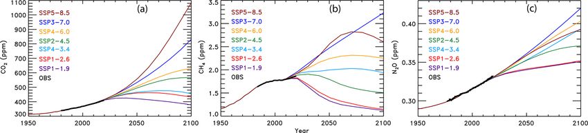
554                             L. A. McBride et al.: Comparison of CMIP6 warming to an empirical model of global climate

timates that seem unreasonably small (see Fig. S10 and the            We calculate AAWR utilizing the EM-GC by computing a
Supplement). Because of the discrepancy in uncertainties be-       linear fit to the 1THUMAN,ATM term,
tween OHC records, we create a new uncertainty time se-
ries using both the 1σ standard deviation of the average of                             1+γ
                                                                   1TATM,HUMAN i =          {GHG 1RFi + AER 1RFi
the five OHC records and the uncertainties from the Cheng                                λp
et al. (2017) (hereafter Cheng 2017) OHC record. We cre-                             +LUC 1RFi − QOCEAN } ,                      (9)
ate this new uncertainty from 1955–2019 through a monthly
time step and use either the 1σ standard deviation of the av-      for a regression that spans 1850–2019. The 1THUMAN,ATM
erage of the five OHC records or the uncertainties from the        term represents the net impact of the change in GMST
Cheng 2017 OHC record, whichever is larger, for that month.        due to RF of climate by anthropogenic GHGs, tropospheric
We use the Cheng 2017 OHC uncertainties because these es-          aerosols, and the variation in surface reflectivity due to
timates are the largest of the five data sets. Additionally, the   land-use change (deforestation), taking into account that for
standard deviation from the mean of the five OHC records is        each model time step, a portion of the human-induced cli-
very low in the 1980s, which is an artifact of our normaliza-      mate forcing is exported to the world’s oceans. For each
tion treatment not inherent to any of the records. This com-       simulation, the slope of the linear least squares fit to the
bined uncertainty estimate is substituted in for each individ-     480 monthly values of 1THUMAN,ATM is used to determine
ual data set and the average, resulting in our use of the same     AAWR. For the time period 1975–2014, a value for AAWR
time-varying uncertainty in OHC for all data sets. Figure S10      of 0.167±0.007 ◦ C per decade is found using a value of AER
and the Supplement provide more detail on the creation of          RF2011 equal to −0.9 W m−2 , wherein the uncertainty cor-
this time-dependent uncertainty estimate for OHC.                  responds to the 2σ standard error of a linear least squares
   The choice of OHC record has only a small effect on fu-         fit. The computation of AAWR found by fitting monthly val-
ture projections of GMST using the EM-GC. Figure 4 illus-          ues of 1THUMAN,ATM is insensitive to modest changes in the
trates the effect of varying the OHC record on future temper-      start and end year for the AAWR calculation (see Table S1).
ature. The bottom boxes in each panel show the observed            The value of λ6 , and therefore AAWR, is also insensitive
and modeled OHC, the value of κ needed to best fit the             to whether or not the AMOC, PDO, or IOD terms are in-
                                                 2
OHC data record, and the resulting value of χOCEAN     . Of the    cluded in the regression framework (Canty et al., 2013; Hope
two OHC records shown, Balmaseda et al. (2013) (Fig. 4a)           et al., 2017). We are able to fit the climate record better (i.e.,
yields the lowest value of κ, and Ishii et al. (2017) (Fig. 4b)    smaller values of χ 2 in Eqs. 6, 7, and 8) by including the
results in the highest estimate of κ. For the same value of        AMOC term. However, computed values of AAWR are in-
AER RF2011 (i.e., −0.9 W m−2 ) and GHG scenario (SSP4-             sensitive to whether the AMOC is used in the regression be-
3.4), we find a difference of 0.25 ◦ C in the modeled rise in      cause whatever contributions the variation in the strength of
GMST in the year 2100 for these two simulations (red lines         the thermohaline circulation may have had on GMST are not
in top boxes). For most of the remaining analysis, we use          considered in Eq. (9) (see Fig. S11 for further explanation).
the multi-measurement average of the five OHC data records.            The determination of AAWR from historical CMIP6
In Sect. 3.1 and 3.2 we quantify the effect of the OHC data        near-surface air temperature output involves conducting a
record on both the attributable anthropogenic warming rate         regression of deseasonalized, globally averaged, monthly
and effective climate sensitivity.                                 1T (1T DES,GLB ) from each GCM (Hope et al., 2017),
                                                                   termed the REG method. The archived CMIP6 historical runs
2.3   Attributable anthropogenic warming rate
                                                                   are constrained by observed variations in SAOD and influ-
                                                                   enced by other factors such as internal model-generated EN-
The attributable anthropogenic warming rate, or AAWR, is           SOs. The 1T DES,GLB time series for all of the runs from each
the time rate of change in GMST due to humans from 1975–           CMIP6 GCM are averaged together to obtain one time series
2014. We use AAWR as a metric in the EM-GC frame-                  of 1T DES,GLB for each GCM. This average 1T DES,GLB time
work to quantify the human influence on global warming             series is used to compute AAWR. The regression approach
over the past few decades and, most importantly, to also as-       is used to compute the influence of SAOD on GMST from
sess how well the CMIP6 GCMs can replicate this quantity.          CMIP6 GCMs. The time needed for GMST to respond to a
This analysis is motivated by the study of Foster and Rahm-        change in the aerosol loading in the stratosphere due to a vol-
storf (2011), who examined the human influence on the time         canic eruption in each GCM can exhibit a significant differ-
rate of change in GMST from 1979–2010 using a residual             ence compared to the empirically determined response time
method. We extend the end year of our analysis to 2014 be-         of 6 months discussed in Sect. 2.1. A lag was determined
cause this is the last year of the CMIP6 historical simula-        for each GCM by calculating the value of the monthly delay
tion. We pushed the start year back to 1975 so that our anal-      between volcanic eruptions and the surface temperature re-
ysis covers a 40-year period, over which the effect of human       sponse that resulted in the largest regression coefficient for
activity on GMST rose nearly linearly with respect to time         SAOD. We regress the 1T DES,GLB against SAOD and the
(Figs. 1b and S10c).                                               anthropogenic effect on temperature, which is approximated

Earth Syst. Dynam., 12, 545–579, 2021                                                 https://doi.org/10.5194/esd-12-545-2021
L. A. McBride et al.: Comparison of CMIP6 warming to an empirical model of global climate 555
Figure 4. Measured (HadCRUT5) and EM-GC simulated GMST change (1T ) from 1850–2019, as well as projected 1T to the year 2100
2
for SSP4-3.4. The top box in each panel shows observed (black) and simulated (red) 1T , the λ6 and χATM values, and the Paris Agreement
target and upper limit. The second row of boxes displays the contribution of GHGs, aerosols, and land-use change to 1T . The bottom boxes
compare the observed (black) and modeled (red) OHC for two different OHC records and display the value of κ needed to provide best fits
2
to the OHC record, as well as best-fit values of χOCEAN . Both use an aerosol RF in 2011 of −0.9 W m−2 . (a) OHC record from Balmaseda
et al. (2013). (b) OHC record from Ishii et al. (2017).
as a linear function from 1975–2014. The value of AAWR is sus REG (see Fig. S14) results in a correlation coefficient
the slope of the anthropogenic effect on temperature. Figure (r 2 ) of 0.995 and a mean ratio of 1.009 ± 0.015, with LIN-
S12 illustrates the REG method used to determine AAWR based AAWR exceeding REG-based AAWR by about 1 %.
from the CMIP6 GCMs. Table S3 depicts the slight effect The close agreement of AAWR found using both methods
on values of AAWR for the CMIP6 GCMs of changing the provides strong evidence for the accurate determination of
start or end year for the regression. At the time of analysis, AAWR from the CMIP6 GCMs. We use the REG method in
there are 50 CMIP6 GCMs with the necessary archived out- this analysis because it provides a more rigorous technique
put to calculate AAWR, with the values of AAWR found us- to remove the influence of SAOD on GMST from the CMIP6
ing REG shown in Table S3. Figure S13 and the Supplement multi-model ensemble compared to the LIN method.
compare values of AAWR found using the REG method ap- The CMIP6 multi-model ensemble provides simulations
plied to EM-GC output with values of AAWR found using of near-surface air temperature (TAS), which we use to calcu-
Eq. (9) as support for the validity of using the REG method late AAWR. The EM-GC uses blended near-surface air tem-
to determine AAWR from CMIP6 output. perature to determine values of AAWR. Cowtan et al. (2015)
We also use a second method to extract the value provide a method to create blended near-surface air temper-
of AAWR from the CMIP6 multi-model ensemble. This ature output from the GCMs. The CMIP6 multi-model en-
method, termed LIN, involves a linear regression of global, semble contains archived fields of TAS and the temperature
annual average values of GMST from the CMIP6 multi- at the interface of the atmosphere and the upper boundary of
model ensemble (Hope et al., 2017). For LIN, we exclude the ocean (TOS) (Griffies et al., 2016), whereas only a subset
the years of obvious volcanic influence on the rise in GMST of GCM groups provide the archived land fraction needed
from the CMIP6 multi-model ensemble historical simula- to calculate blended near-surface air temperature using the
tions: i.e., data for 1982 and 1983 (following the eruption Cowtan et al. (2015) method. Cowtan et al. (2015) compared
of El Chichón) and 1991 and 1992 (following the eruption of the modeled and measured trend in global temperature over
Mount Pinatubo) are excluded. Archived global, annual av- 1975–2014 and found a 4.0 % difference in the trend upon the
erage values of GMST covering 1975–2014, excluding these use of blended temperature from CMIP5 GCMs rather than
4 years, are fit using linear regression, with the AAWR set global modeled TAS. Their analysis focused on a compari-
equal to the slope of the fit. Values of AAWR for 1975– son of modeled and measured temperature, not just the an-
2014 found using LIN are also shown in Table S4 for each thropogenic component. We have used the method of Cow-
GCM. Analysis of AAWR for these 50 GCMs of LIN ver- tan et al. (2015) to create blended CMIP6 temperature out-
https://doi.org/10.5194/esd-12-545-2021 Earth Syst. Dynam., 12, 545–579, 2021556 L. A. McBride et al.: Comparison of CMIP6 warming to an empirical model of global climate
put for the CMIP6 GCMs that provide TAS, TOS, and the ulations persist until equilibrium. At the time of this analy-
land fraction. Upon our use of blended CMIP6 temperature sis, 28 models released the necessary output to the CMIP6
output for these GCMs and calculation of AAWR for 1975– archive (see Table S5 for the list of models and individual
2014, we find that AAWR based on blended CMIP6 tempera- values of ECS). Several recent analyses suggest the Gregory
ture is 3.5 % lower than AAWR found when using only TAS. method underestimates the true value of equilibrium climate
Tokarska et al. (2020b) estimate an effect of 0.013 ◦ C per sensitivity from the CMIP6 multi-model output (Rugenstein
decade in the trend of CMIP6 temperature output upon the et al., 2020; Sherwood et al., 2020; Zelinka et al., 2020).
use of blended CMIP6 temperature instead of TAS, while However, effective climate sensitivity is strongly correlated
Cowtan et al. (2015) report a difference of 0.030 ◦ C per with the amount of warming simulated by GCMs for high
decade between the trend in observations and modeled out- carbon emission scenarios and is more relevant for warm-
put. Since the difference between values of AAWR found us- ing over the timescale of interest (rest of this century) due to
ing blended CMIP6 temperature output and TAS is so small the long time needed to achieve equilibrium (Sherwood et al.,
and does not affect any of our conclusions, we use TAS out- 2020). We use the Gregory method to calculate ECS from the
put from the CMIP6 multi-model archive because this choice CMIP6 GCMs because this procedure is preferred by Eyring
allows many more GCMs to be examined. et al. (2016) for use within the CMIP6 community.
The estimates of climate sensitivity from Eq. (10) and
2.4 Effective climate sensitivity those found using the Gregory et al. (2004) method are
termed “effective” because they assume that climate feed-
The equilibrium climate sensitivity represents the warming back inferred from either the historical climate record or the
that would occur after the climate equilibrated with atmo- abrupt 4× CO2 experiment persists until equilibrium. How-
spheric CO2 at the 2× pre-industrial level (Kiehl, 2007; Otto ever, these estimates of ECS differ in that the perturbation to
et al., 2013; Schwartz, 2012). In our model framework, we the RF of climate over the historical record is considerably
infer the climate sensitivity based on an estimate of climate smaller than the RF of climate that underlies the 4× CO2 ex-
feedback from the historical record, resulting in the effective periment of the Gregory et al. (2004) method. We quantify
climate sensitivity (ECS) (Tokarska et al., 2020a). Effective the impact of time-variable climate feedback on climate sen-
climate sensitivity is defined by IPCC 2013 as “an estimate sitivity in Sect. 3.3.6.
of the global mean surface temperature response to doubled
carbon dioxide concentration evaluated from model output
or observations for evolving non-equilibrium conditions”. To 2.5 Aerosol weighting method
calculate ECS from the EM-GC, we use Probabilistic forecasts of the future rise in GMST for var-
1+γ ious SSPs are an important part of our analysis. Probabil-
ECS = × 5.35 W m−2 × ln (2) , (10) ities of AAWR and ECS are computed by considering the
λP
uncertainty in AER RF2011 . We also provide probabilistic es-
which represents the rise in GMST for a doubling of CO2 , as- timates of AAWR and ECS. All of these quantities are com-
suming no other perturbations and equilibrium in other com- puted by incorporating the uncertainty in the radiative forc-
ponents of the climate system (i.e., QOCEAN = 0) (Mascioli ing of climate due to tropospheric aerosols within results of
et al., 2012). The expression for the radiative forcing of CO2 our EM-GC simulations. We use an asymmetric Gaussian to
is from Myhre (1998). The quantity γ in Eq. (10), which assign weights to the value of GMST, AAWR, or ECS found
represents the sensitivity of the GMST to feedbacks within for various time series of radiative forcing by aerosols as-
the climate system, is the only variable component of ECS. sociated with particular values of AER RF2011 . Figure 5a
We only use values of γ that result in good fits (χ 2 ≤ 2 for shows the asymmetric Gaussian function we use to maxi-
Eq. 6 to 8) between modeled and observed GMST and mod- mize the values of AAWR or ECS at the best estimate of
eled and observed OHC. We refer to the quantity in Eq. (10) AER RF2011 of −0.9 W m−2 , accomplished by giving these
as effective climate sensitivity, rather than equilibrium cli- values the highest weighting. The IPCC 2013 “likely” range
mate sensitivity, because for most of our analysis we assume limits of AER RF2011 of −0.4 and −1.5 W m−2 (Myhre et
a constant value of climate feedback inferred from prior ob- al., 2013) are assigned to the 1σ values of the Gaussian, and
servations. the AAWR or ECS estimates occurring at the “likely” range
For the estimate of climate sensitivity from the CMIP6 AER RF2011 limits are given the same weighting. The −0.1
multi-model ensemble, we use the method described by Gre- and −1.9 W m−2 limits of the AER RF2011 range are as-
gory et al. (2004) (see the Supplement and Fig. S15 for more signed as the 2σ values of the asymmetric Gaussian based on
information). The Gregory et al. (2004) method also esti- the IPCC 2013 description of these two values as being 5 %
mates effective climate sensitivity from the CMIP6 GCMs and 95 % uncertainty limits (Myhre et al., 2013). The Gaus-
(Gregory et al., 2004; Sherwood et al., 2020; Zelinka et al., sian we use is asymmetric due to the fact that the distribution
2020) because it assumes that the feedbacks inferred from of the likely range and the 5th and 95th percentiles of the val-
the first 150 years of the abrupt 4× CO2 CMIP6 GCM sim- ues of AER RF2011 are not distributed symmetrically from
Earth Syst. Dynam., 12, 545–579, 2021 https://doi.org/10.5194/esd-12-545-2021You can also read