Data-driven simulation in fluids animation: A survey - Virtual ...
←
→
Page content transcription
If your browser does not render page correctly, please read the page content below
Virtual Reality & Intelligent Hardware       2021 Vol 3 Issue 2:87—104

·Review·

Data-driven simulation in fluids animation: A survey
Qian CHEN, Yue WANG, Hui WANG, Xubo YANG*
School of Software, Shanghai Jiao Tong University, Shanghai 200240, China

* Corresponding author, yangxubo@sjtu.edu.cn
Received: 10 December 2020      Accepted: 2 February 2021

Supported by the Natural Key Research and Development Program of China (2018YFB1004902); the Natural Science Foundation of
China (61772329, 61373085).

Citation: Qian CHEN, Yue WANG, Hui WANG, Xubo YANG. Data-driven simulation in fluids animation: A survey. Virtual
           Reality & Intelligent Hardware, 2021, 3(2): 87—104
           DOI: 10.1016/j.vrih.2021.02.002

Abstract       The field of fluid simulation is developing rapidly, and data-driven methods provide many
frameworks and techniques for fluid simulation. This paper presents a survey of data-driven methods used
in fluid simulation in computer graphics in recent years. First, we provide a brief introduction of physical-
based fluid simulation methods based on their spatial discretization, including Lagrangian, Eulerian, and
hybrid methods. The characteristics of these underlying structures and their inherent connection with data-
driven methodologies are then analyzed. Subsequently, we review studies pertaining to a wide range of
applications, including data-driven solvers, detail enhancement, animation synthesis, fluid control, and
differentiable simulation. Finally, we discuss some related issues and potential directions in data-driven
fluid simulation. We conclude that the fluid simulation combined with data-driven methods has some
advantages, such as higher simulation efficiency, rich details and different pattern styles, compared with
traditional methods under the same parameters. It can be seen that the data-driven fluid simulation is
feasible and has broad prospects.

Keywords         Fluid simulation; Data driven; Machine learning

1     Introduction
Fluid simulations have been applied widely in computer graphics. Instead of discrete models, including the
particle Bhatnagar-Gross-Krook[1], particle Fokker-Planck[2], direct simulation Monte Carlo-computational
fluid dynamics (CFD) hybrid[3], multiscale particle[3], and coarse-grained particle simulation methods[4], we
focus primarily on a continuum model governed by the well-known Navier-Stokes (N-S) equation that is
the mainstream model in computer graphics. To simplify the physical model, the mass conservation of a
constant density field is typically enforced under the incompressibility assumption for water and smoke
animation. In addition, other physical forces, such as surface tension, viscosity, and vorticity, yield
interesting phenomena to fluid simulations.
    The underlying discretization used in physical-based simulations ranges widely from Lagrangian
particles and meshes to the Eulerian grid. By mapping a continuous fluid onto these structures, the fluid is

2096-5796/©Copyright 2021 Beijing Zhongke Journal Publishing Co. Ltd., Publishing services by Elsevier B.V. on behalf of KeAi Commu‐
nication Co. Ltd. This is an open access article under the CC BY-NC-ND license (http://creativecommons.org/licenses/by/4.0/).

                                                                                                                      www.vr-ih.com
Virtual Reality & Intelligent Hardware   2021 Vol 3 Issue 2:87—104

tracked or observed by the discrete degrees of freedom in which those partial differential equations (PDEs)
are solved to apply the physical force. To achieve better stability and accuracy, these constraints are
typically solved implicitly, resulting in a large linear system to be solved using numerical solvers.
     The contradiction between high resolution and high performance is a key issue in physical simulations.
Typical approaches for improving performance include adaptivity[5-7], model reduction[8], and using
accelerated solvers[9,10]. Other methods focus on small-scaled details, including turbulence synthesis[11],
vortex sheets[12], turbulence particles[13], and multiscale solvers[14]. In these methods, solutions are proposed
based on the white-box modeling of the problem; hence, their applicability might be limited.
     Recently, emerging demands such as motion control, artistic stylization, and animation synthesis have
resulted in high requirements for the simulation framework. In these applications, it is challenging to
design intricate methods to satisfy the constraints or define the constraint explicitly.
     Owing to rapid developments over the past decade, the data-driven method has become more effective
and hence has been used widely in computer vision (CV) and natural language processing tasks. The data-
driven method, particularly the machine learning (ML) method, relies on a large amount of historical data
to build a mathematical model; it generates predictions based on the knowledge learned automatically from
training. Treuille et al. first introduced the data-driven method into fluid simulation using a dimension
reduction method to accelerate the complex fluid dynamic system[15]. Other data-driven models, including
state graphs[16], regression forests[17], and neural networks[18‒21], have been applied to predict fluid evolution
without numerical simulation. Based on CV concepts, data-driven methods provide new tools for studies
associated with solver acceleration and detail enhancement, including autoencoders[19], long short-term
memory (LSTM) [22], generative adversarial networks (GANs) [23], and continuous convolution[24]. Furthermore,
they have prompted a broad array of applications of fluid simulation, such as fluid-style transfer[25,26], fluid
reconstruction[27], game control[28], and turbulence modeling[29]. Compared with previous studies that
summarize the use of data-driven methods in physical-based modeling[30,31], this survey primarily focuses
on the integration of ML techniques in fluid simulation in computer graphics.
     In this survey, we briefly introduce physical-based simulations for fluid animation in Section 2. Three
sets of simulation results using traditional methods are shown in Figure 1. Section 3 describes the data-
driven methodologies used in Eulerian, Lagrangian, and hybrid viewpoints as well as issues associated
with spatial discretization. Several mainstream applications are reviewed in Section 4, including data-
driven solvers, detail enhancement, animation synthesis, fluid control, and differentiable simulation.
Typical technical issues in data-driven fluid simulations are discussed in Section 5.

Figure 1    Fluid simulation results using physical-based methods. Left: smoke interacting with a sphere in Eulerian
method[32]. Middle: liquid collides with the column in Lagrangian method[33]. Right: waterwheels transport water in
hybrid method[34].

2      Physical-based fluid simulation method
The incompressible fluid is governed by the well-known Navier-Stokes equation, which describes the fluid
88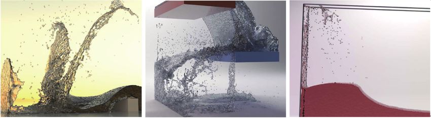
Qian CHEN et al: Data-driven simulation in fluids animation: A survey

evolution in a continuous field during the simulation. Equation (1) shows the incompressible N-S equation.
                                           Du              ∇p
                                              = υ∇ ⋅ ∇u -      + f,
                                           Dt               ρ                                               (1)
                                           ∇⋅u=0
where u denotes the vector field of velocity, υ the viscosity coefficient, ρ the density, p the scalar field of
pressure, and f the body force. The first equation describes the momentum changes caused by viscosity,
pressure, and body force. The second equation enforces the divergence-free condition on the velocity field
to achieve incompressibility. A compressible variant can be derived based on the conservation of mass[35].
In computer graphics, the N-S equation is solved by discretizing the continuum from differential
viewpoints, which will be discussed below.

2.1   Eulerian method

In the Eulerian method, fluid is observed at static points. It was first introduced into graphics by Foster et
al. [36], and Stam[37] further improved its stability by introducing a semi-Lagrangian advection step. In
Foster's and Stam's models, a fluid is discretized on a static unified grid. The physical properties are stored
on the grid nodes and grid faces of a marker-and-cell (MAC) grid[38]. Subsequently, differential stencils are
built on adjacent cells base on the center-differential scheme. The time integration in the Navier-Stokes
equation is segregated and solved step by step. Specifically, the projection term is solved implicitly as a
global Poisson equation of the pressure field, and it is typically the bottleneck of the entire simulation
pipeline. A set of adaptivity strategies, including tall cells[39], far-field grids[40], Octree[5], and adaptive
staggered-tilted grids[41], was proposed to capture more small-scale details in the region of interest while
reducing the overall number of degrees of freedom.

2.2   Lagrangian method

The smoothed particle hydrodynamics (SPH) method was first proposed by Monaghan et al. [42] and applied
to an interactive application by Müller et al.[43]. Macklin et al. further used the SPH kernel in position-based
dynamics (PBD) [44], which is widely used in real-time multimaterial applications[45], to simulate a position-
based fluid.
  Lagrangian particles achieve mass conservation naturally while differential operators are harder to
construct. Therefore, most of the differential stencils rely on the neighboring searching operation to
approximate a local continuous field. In SPH, differentiation is performed on neighboring particles using a
smooth kernel that weights particles around in its region. Cornelis et al. [46] and Bender et al. [33] further
solved the instability problem and achieved incompressibility. Similar meshless differentiation methods
can be seen in reproducing kernel particle methods[47] and the element-free Galerkin method[48].

2.3   Hybrid method

The hybrid method incorporates both the Eulerian and Lagrangian methods, in which a structured grid is
used for differentiation and geometry tracking for thin feature preservation. The basic idea is to perform
kinematic procedures on particles and dynamic steps on the static grid simultaneously. Meanwhile, a
particle-grid interpolation is used to transfers the physical properties back and forth.
  Harlow et al. first applied the particle-in-cell (PIC) method to fluid simulation, in which excessive
numerical dissipation is introduced[49]. Based on the PIC method, Brackbill et al. proposed the fluid implicit
particle (FLIP) method, which transfers the update of the velocity field instead of itself to attenuate the
                                                                                                                          89
Virtual Reality & Intelligent Hardware   2021 Vol 3 Issue 2:87—104

numerical dissipation[50]. Zhu further combined these two methods with a blending factor[51]. Jiang et al.
achieved a grid-particle interpolation step using an affine descriptor[52], whereas Fu et al. [53] and Hu et al. [34]
improved energy and vorticity conservation by augmenting each particle with a polynomial and moving
least square descriptor during particle-grid interpolation.
     Compared with the pure Eulerian method, the hybrid method reduces the numerical dissipation
introduced by grid interpolation during the advection step and achieves mass conservation naturally with
particles. Compared with the Lagrangian method, it solves the implicit constraints with a global linear
system defined on a regular structure and improves the accuracy.

3      Data-driven methodology
In this section, we introduce data-driven methods based on different spatial discretizations and discuss the
underlying connection between fluid simulation and the data-driven method.

3.1     Eulerian data-driven methods

We first limit our discussion to the regular grid used in existing data-driven methods. The Eulerian method
primarily uses the central difference scheme to discretize the differential operators on adjacent cells. The
local data-driven solver based on the descriptor of adjacent cells is inspired by the Eulerian method. For
example, Yang et al. proposed a patch-based projection artificial neural network solver with a local
descriptor on each cell containing the local pressure, cell type, and velocity divergence of neighboring
cells. A similar concept was used in the detail synthesis[54]. Chu et al. trained a patch-based convolutional
descriptor to locally synthesize high-resolution details from their space-time flow repositories[55]. The
synthesis results are shown in Figure 2.

Figure 2    Smoke synthesis results using CNN[55]. Left: low-resolution baseline. Right: high-resolution synthesized smoke.

     In addition, the global data-driven method regards the entire fluid field as the input. Owing to the
structural similarity between the Eulerian field and image, and the receptive field similarity between the
convolution kernel and central difference scheme, a model based on a convolution neural network (CNN)
that is typically used by the CV community has been introduced to the data-driven Eulerian solver[18,56,57].
     In terms of three-dimensional (3D) simulation, the space complexity of a global input increases
cubically with the field length, necessitating feature extraction or input segmentation methods. In earlier
studies[15,58], principal component analysis was used to extract features. However, owing to its poor
90
Qian CHEN et al: Data-driven simulation in fluids animation: A survey

adaptivity to nonlinear problems, solutions with data-driven methods are often pursued. For example, Ling
et al. embedded Galilean invariance extracted from original data fields into Reynolds stress anisotropy
predictions to improve Reynolds-averaged Navier-Stokes (RANS) turbulence models[59]. Xiong et al.
proposed a learning-based framework to extract discrete Lagrangian vortex particles as features from a
continuous Eulerian flow field[60]. Currently, some researchers[19,22,28,61‒63] combine the architectures of
autoencoders in deep learning to obtain more effective feature representations.

3.2    Lagrangian data-driven methods

Unlike the regular grid, Lagrangian particles are unstructured, rendering network modeling challenging.
Stanton et al. were the first to propose a precomputed state graph for real-time fluid simulation, in which
each graph vertex represents particle positions and velocities in one frame, and one edge represents a short
transition between states[16]. Meanwhile, one of the most important characteristics of the Lagrangian
method is local differentiation based on neighboring particles. The regression forest method is based on the
state graph. It constructs regression trees by applying particles distribution and the velocity of neighboring
particles as node attributes. Using the state of neighboring particles as input, the future motion state of the
central particle is predicted by traversing the trees[17]. Regarding the similarity between unordered
Lagrangian particle sets and the point cloud model, ideas from point cloud processing have been adopted
in the Lagrangian system in a few cross-disciplinary studies. The continuous convolution (CConv)
method[64] proposes a point cloud based convolutional operation with a spherical filter. Ummenhofer et al.
integrated the network into a fluid simulation by applying a convolution operator on both fluid and
boundary particles in the neighborhood under the SPH framework[24]. Their water simulation results
compared with those of divergence-free smoothed particle hydrodynamics (DFSPH) [65] are shown in Figure
3. In the graph-based network[66,67], in terms of frequent geometry changes in the fluid, researchers must
dynamically build edges in the graph between neighboring particles and extract topological features using
graph convolution. Schenck et al. proposed a novel model known as SPNets, in which a ConvSP layer is
constructed to compute fluid-particle-particle pairwise interactions, and a ConvSDF layer to compute
particle-static-object interactions[68].

   Figure 3   Water simulation using CConv[24]. Top row: results from CConv. Bottom row: results from DFSPH[65].

3.3    Hybrid data-driven methods

In hybrid fluid simulation, data-driven optimization can be applied to either Lagrangian particles or the
Eulerian grid.
  For the data-driven solver, similar to the Eulerian method, neural network models are often used to
replace the time-consuming procedures. In a previous study[69] based on the material point method, the
                                                                                                                           91
Virtual Reality & Intelligent Hardware 2021 Vol 3 Issue 2:87—104
internal acceleration calculation in particles was replaced with a neural network. For the detail synthesis,
particle-based reseeding is a better option. Neural network models can be used to modify physical
variables in regions of interest to enrich fluid details under low resolutions. For example, the machine
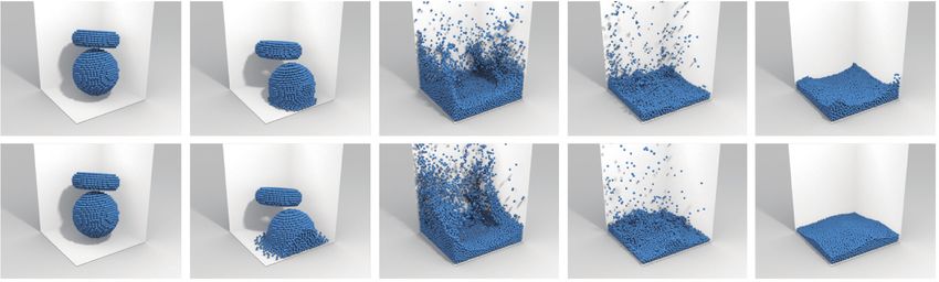
learning FLIP (MLFLIP) [70] can model the splashing details in the FLIP framework as a probability
distribution problem with two networks, the simulation results of which are shown in Figure 4. In this
example, a classifier was trained to identify the splashing details of the fluid, and the splash particle
velocity was sampled using a modifier that inferred a normal distribution for small-scale details.
Figure 4 Several simulation scenes using MLFLIP[70]. Left: dam break. Middle: water flowing down the stairs.
Right: wave tank.
4 Application
In this section, we present a wide range of applications of data-driven methods in fluid simulation,
including data-driven solvers, detail enhancement, animation synthesis, fluid control, and differentiable
simulation.
4.1 Data-driven solver
For the Eulerian method, some data-driven solvers have been proposed to replace the time-consuming
projection procedure in the Eulerian method particularly to replace the numerical solver of the Poisson
equation. Yang et al. proposed an artificial neural model for Poisson solving[54]. Subsequently, convolution-
based projection solvers were used by Tompson et al. [18] and Xiao[56,57,71]. Others focused on the temporal
continuity of the fluid field and modeled the time evolution of the field by introducing the recurrent neural
network (RNN) structure and generative models. Wiewel et al. proposed an LSTM-based model with
convolutional layers that can model projection solving with the pressure field as input, as well as model the
entire simulation loop as the evolution of velocity fields[61]. Kim et al. encoded a physical simulation in
their generative network model, which can generate plausible fluid results with divergence-free velocities
under different parameters (Figure 5 (left))[62].
For Lagrangian particles, precomputed graphs[16,17] constructed with global or local particle distributions
were proposed for motion prediction (Figure 5 (right)). To model the interparticle interaction force in the
Lagrangian system, Battaglia et al. introduced an interaction network in a rigid-body simulation[72]. Li et al.
developed dynamic particle interaction (DPI) networks that captured the dynamic, hierarchical, and long-
range interactions of particles for fully learning particle dynamics[66]. This particle-based simulator can be
applied to multimaterial scenarios. Sanchez-Gonzalez et al. [67] referred to graph networks (GNs) [73] and
proposed the graph network-based simulator (GNS) to perform predictions in particle-based simulations.
Compared with previous approaches, including DPI[66] and the GN-based model[73], the GNS method is
simpler for simulation while affording better generalization. In addition, the continuous convolution
92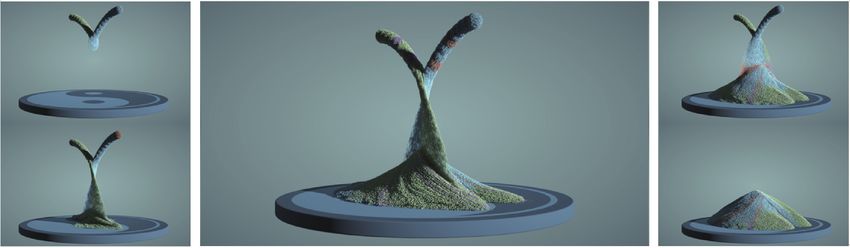
Qian CHEN et al: Data-driven simulation in fluids animation: A survey

Figure 5   Simulation results with data-driven solver. Left: water interacts with rigid objects[17]. Right: smoke simulation[62].

method models the convolution operation on point clouds in a connection-free manner, and it can be
regarded as an extension of the SPH operation. Ummenhofer et al. used spatial convolution to connect each
liquid particle with its neighbors and obtained position correction by the continuous convolution of
neighboring particles[24]. Mukherjee et al. used an LSTM-based RNN framework to replace the calculation
of color field gradient at the droplet's contact front to address microscopic forces and boundary conditions
when simulating small-scale fluids[74].

4.2   Detail enhancement

In contrast to the data-driven solver, detail enhancement adds fine detailed features to the physical field or
visual result based on a coarse numerical simulation. It can be categorized into three major aspects: detail
synthesis, super-resolution, and style transfer.
  For a data-driven detail synthesis, a data repository of high-resolution details is typically used. During
the simulation, those details are mapped to the corresponding patch on a low-resolution fluid for detail
generation. Sato et al. synthesized small-scale details for 3D low-resolution fluid velocity fields in a patch-
based manner by constructing a precomputed database of two-dimensional (2D) high-resolution fluid
velocity fields and applying them in the advection step[58]. They improved their method by enriching low-
resolution target smoke to one with turbulence details and using an optimization-based synthesis method to
resolve the discontinuity between patch boundaries[75]. Chu et al. trained a CNN indicator to encode the
similarity between fluid regions of different resolutions. Using this indicator, they successfully matched
their simulation data to their reusable repositories of space-time flow data to optimize the visual results
efficiently[55]. By contrast, Um et al. synthesized splashing droplets in the FLIP framework by first
identifying the surface particles and predicting their velocities using a splashing distribution model[70].
  As suggested by its name, "super-resolution" upscales the input flow field and recovers the high-
resolution flow field by inferring the subgrid details in the original field. Xie et al. generated high-
resolution fields from 3D volumetric smoke data using a GAN model with a temporal discriminator to
maintain consistency in the details over time and a spatial discriminator to preserve the details of high
spatial frequencies, whose super-resolution results are shown in Figure 6[23]. Werhahn et al. improved
scalability by decomposing the learning problem into multiple smaller subproblems[76].
  In digital images and videos[77‒79], a style is transferred by generating a blending result containing the
style of one input and the content of the other. Combined with fluid dynamics, style transfer creates
interesting and impressive results. Kim et al. proposed a transport-based neural style transfer (TNST)
model based on the Eulerian viewpoint[25]. They designed a differentiable renderer to stylize 3D smoke
using 2D images ranging from simple patterns to intricate motifs. Subsequently, they extended their study
                                                                                                                                 93
Virtual Reality & Intelligent Hardware    2021 Vol 3 Issue 2:87—104

Figure 6     Super-resolution smoke using GAN[23]. Left: low-resolution smoke. Right: low-resolution smoke passed
through GAN.

to the Lagrangian representation by adding an additional transfer step between the particle and grid[26]. This
method eliminated the expensive recursive alignment and ensured better time consistency than TNST.

4.3     Animation synthesis

In animation synthesis, the space-time evolution of a fluid is not solved explicitly but is predicted by the
model based on the input. Interpolation-based methods generate animation with several specified
animations by defining a smooth interpolation mapping between them. Thuerey used a keyframe-based
method to interpolate a dense space-time deformation using an optical flow solver combined with a
projection algorithm that recovered small-scale details[80]. Pan et al. used keyframe interpolation to generate
fluid fields in between keyframes by obtaining the local driving force field of each frame through their
space-time optimization method constrained by partial differential equations[81]. Sato et al. synthesized fluid
animation by combining existing flow data in different scenarios. They defined an interpolation function to
adjust the velocity at the boundary of different flow fields to obtain a natural combination with different
flow fields[82].
     For fluid reconstruction from video, Eckert et al. reconstructed a time-consistent flow field from a real-
world smoke video, as shown in Figure 7, and proposed the estimation of the unseen flow region and an
optimization scheme constrained by the real fluid[27]. They first initialized the density with a single pass of
regular tomography and a velocity of zero; subsequently, they calculated the residual velocity that is
necessary to match the motion and shape from the input image sequence, and the density inflow, while
preserving the divergence-free constraint.

                           Figure 7      Reconstructed smoke from real-world smoke videos[27].

4.4     Fluid control

Fluid control primarily includes fluid editing, shape correction, and fluid motion control. For fluid editing,
Flynn et al. applied the seam carving method from image processing to the post-processing of fluid
94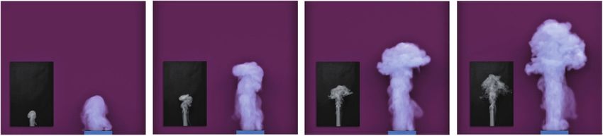
Qian CHEN et al: Data-driven simulation in fluids animation: A survey

animation, the results of which are shown in Figure 8[83]. They defined a graph cut energy function based on
the average curvature and kinetic energy; subsequently, the function was used to add or remove seams for
the flow field to ensure the consistency of the content after the flow was resized. For shape correction,
Nielsen et al. adopted the shape guidance method by adding constraints to guide a high-resolution fluid
with a thin outer shell of liquid into a low-resolution fluid with a thicker shell of liquid to retain the low-
resolution shape features in the high-resolution scene[84]. For fluid motion control, Ma et al. addressed fluid-
solid coupling control in a data-driven manner[28]. They applied reinforcement learning to a game of jetting
water onto a ball by inputting a combination of rigid body features and fluid features extracted using an
autoencoder. Morton et al. transformed the original flow field coordinate into a new one using an encoder-
decoder scheme to control vortex shedding suppression[85]. Holl et al. designed a control network that can
be used to infer the control parameters to control fluid shape transformation[86].

Figure 8   Water surface can be intelligently resized in rain simulation using seam carving methods[83]. Left: water
surface by removing several seams. Middle: original water surface. Right: water surface by adding several seams.

4.5   Differentiable simulation

Differentiability has been widely investigated in recent years; it enables the derivative of a function to be
evaluated numerically. By applying differentiability to a physical simulation, a simulator can be
incorporated into the gradient-based optimization algorithm as well as combined with ML algorithms to
effectively solve inverse problems. Schenck et al. proposed a differentiable fluid solver SPNets that can
learn liquid parameters from data and perform liquid control tasks[68]. They added two new layers to the
deep neural network (DNN) model: ConvSP and ConvSDF. The ConvSP layer was designed to compute
the pressure correction solution in the PBF, whereas the ConvSDF layer was designed specifically to solve
particle-static-object collisions. Hu et al. built a differentiable simulator for soft robotics to solve a series of
inference, control, and collaboration tasks[87]. In addition, they integrated differentiability into the high-
performance Taichi[88] framework (Figure 9), enabling differentiability for a rigid body, soft body, fluids,
etc. [89]. In addition, Holl et al. designed a predictor network to plan the optimal trajectory and a control
network to infer control parameters based on a differentiable simulator[86].

                              Figure 9   Sand jet animation using Taichi framework[88].

                                                                                                                            95
Virtual Reality & Intelligent Hardware 2021 Vol 3 Issue 2:87—104
5 Technical issues and future directions
This section summarizes the typical technical issues from the various applications presented in Section 4.
These issues necessitate future investigations.
5.1 Interpretability
The interpretability of the models, as a crucial problem in data-driven methods[29], has been discussed by
Lipton[90]. Without interpretability, the data-driven method is a black-box model, whose validity is not
guaranteed. He et al. investigated the relationship between a DNN and the linear finite element method to
demonstrate the potential of the DNN in solving partial differential equations[91]. In their later publication,
they discussed the close connection between the CNN and the multigrid method[92]. Yang et al. used a
differentiable neural structure to learn a wide range of physical constraints, including rigid body rotations,
rope, articulated body, collision, and contact[19].
5.2 Physical fidelity
Physical fidelity is achieved naturally by the law of physics in the physical-based method. By enforcing
these constraints in the numerical algorithm, the fluid behaves the same as in the real world. However, in
data-driven methods, fluid evolution is inferred based on historical data without physical constraints; this
may result in deficient fidelity and visual artifacts.
To render ML models consistent with physical laws, physical knowledge has been incorporated into loss
functions to enable models to capture generalizable dynamic patterns[31]. Notably, embedding the physical
constraints, particularly the incompressibility, into the loss function is a typical approach in the Eulerian
framework[56,57,71]. Kim et al. iteratively designed a loss function, which embedded incompressibility, better
velocity extrapolation, and velocity gradients into their loss function[62].
Another approach for physics-based modeling is to design the network architecture based on physical
models[31]. Owing to similarity in discretization, the CNN and continuous convolution network were used in
the Eulerian and Lagrangian frameworks, respectively[24,56,57]. In addition, considering the spatial continuity
of fluid simulation, the RNN is typically used for the prediction of consecutive frames[22,61,74].
In terms of generative models, Xie et al. introduced TempoGAN, which can generate high-resolution
fields from 3D volumetric smoke data using the GAN with an additional discriminator network[23].
Werhahn et al. designed a temporal and spatial discriminator in a GAN to guarantee the time and space
consistency of smoke to improve the physical fidelity in data-driven simulations[76]. More details regarding
data-driven physics-based modeling are provided in[30,31].
5.3 PDE solving
As mentioned above, the data-driven solvers[18,54,56] demonstrate the potential ability of data-driven models
for solving regular PDEs of the Poisson equation. Solving high-dimension PDEs with a low computation
cost has been a longstanding problem. The data-driven method was leveraged in the numerical solver by
Lagaris et al. [93]. Subsequent studies extend the data-driven PDE solver to higher-dimensional PDEs using
deep learning techniques[94,95]. Another approach to address this issue is to enhance the numerical solver
with a data-driven network; in this approach, convergence and correctness can be achieved easily using the
base of the numerical solver[96]. By integrating an additional learned correction step into the differentiable
pipeline to interact with the solver, Um et al. reduced numerical errors that were disregarded by the PDE
96Qian CHEN et al: Data-driven simulation in fluids animation: A survey
solver[97]. This idea was adopted in the multigrid solver as well, where the network learns the optimal
prolongation and restriction matrices[98,99]. In other studies, a network was proposed to learn the differential
operator and uncover the underlying PDEs. For example, PDE-Net[100] learns the differential operators and
the response function to uncover the underlying PDE.
5.4 Performance optimization
Parallel algorithms have been investigated in various fields of computer graphics[101‒103], including a CPU's
multithreading and a GPU's parallel computing. They have been widely used in parallel training[104] and
extended to physical calculations[105‒108] for acceleration.
In addition, Hu et al. designed an optimized compiler based on the characteristics of data structures and
typical operations in a simulation to solve equations in a sparse computational domain[88]. Furthermore,
they developed a differentiable programming language for simulation, thereby enabling task optimization,
such as motion learning and motion control[89]. Additionally, such studies reveal a new research direction
for optimizing the calculation at the operating system level, in which data-driven training processes can be
accelerated or simulation processes regarded as data-driven optimization iterations.
5.5 Generalization
Generalization is an important indicator for evaluating data-driven models. Without generalization, the
model tends to overfit, which is typically caused by limited data or complex network structures. In fluid
simulation, generalization renders the model applicable to a broad range of fluid scenarios. Xiao et al.
employed the incremental learning technique for a data-driven solver to improve generalization[56]. They
evaluated the error between the network output and physical result for several frames. When the error
exceeded a threshold, an online-learning loop was executed to fine-tune the trained model with the current
scene.
5.6 Model reduction
Model reduction is a typical method for feature extraction in computer graphics and was first introduced to
fluid simulation by Treuille et al. [15]. The main idea is to simplify the model for low computational
complexity while preserving the features as much as possible. Wiewel et al. designed a CNN-based LSTM
to extract fluid features in a latent space[61]. They further segmented their latent space into individual
quantities, enabling them to alter the reductive quantities in the latent space without interfering with
others[22].
5.7 Data processing
It is difficult to predict physical fields credibly by merely applying learning methods from raw fluid data[29].
Researchers often categorize the learning task into data processing, modeling, and evaluation. Among
them, data processing is a basic yet significant task in data-driven fluid simulation methods for providing
reasonable features to data-driven models. It includes fluid feature extraction, selection, identification, and
measurement.
For feature extraction, spatial features are typically extracted from high-dimensional and complex fluid
fields. For example, an autoencoder is used for encoding high-dimensional features into a latent space by
training[22,28,61]. Xiong et al. extracted vortex features from a complex grid-based velocity field and
97Virtual Reality & Intelligent Hardware 2021 Vol 3 Issue 2:87—104
represented vortices using learned Lagrangian particles, as discussed in Section 3.1[60].
For feature selection, Wang et al. adopted random forest regression to predict Reynolds stress
discrepancies in RANS-based turbulence models, in which mean flow features, which comprised the
curvature, gradient of pressure, ratio of turbulence production/dissipation, etc., were used as the input[109].
Milani et al. used the random forest model to predict the turbulent diffusivity field in film cooling flows[110].
They adopted the feature selection proposed by Ling[59] with an additional feature importance evaluation
based on frequency.
For feature identification, Bao et al. preprocessed the input features of a model via feature identification,
which includes feature defining, ranking, and optimization. They defined derivatives of variables and local
physical parameters as features, ranked them using random forests, and optimized feature selection based
on the normalized root mean square error and computational costs[111].
For feature measurement, the global distance error of data fields alone cannot be used to measure the
similarity of local features. As for some structured data, such as grids, image similarity metrics can be
borrowed from CV, and spatial operators such as convolution can be used to extract features for comparison.
For some unstructured data, such as particles, neighborhood search operators can be used to extract spatial
features for comparison. For example, Bao et al. designed a feature similarity measurement (FSM) to estimate
the error in two-phase flows[111]. In addition, to overcome the difficulty of independently evaluating the mesh
effect or model scalability in thermal-hydraulic simulations, Bao et al. proposed a data-driven approach based
on FSM[111] to quantify the uncertainty simulation error by investigating the local similarity in multiscale data
using ML[112]. Similarly, Kohl et al. proposed a stable and generalizing metric known as LSiM using a Siamese
architecture to measure the similarities between two fluid fields or reality scenes[113].
5.8 Dataset framework
The dataset is the foundation for model training and evaluation. In CFD, Li et al. archived a dataset
containing isotropic forced turbulence with the form of a time series of velocity and pressure fields, which
has been widely used for turbulence modeling[114]. In addition, several CFD and fluid datasets including
THT Lab (Myong et al.)[115], KTH Flow (Schlatter et al.)[116], and FDY DNS (Avsarkisov et al.)[117] only offer
single simulated datasets with different resolutions. To provide numerous datasets for a single
phenomenon, Eckert et al. constructed a comprehensive smoke plume dataset[27], which included the
velocity field, density field, calibration data, rendered pictures, and videos, to satisfy the requirements of
some reconstruction-from-video works[118,119]. Recently, a fully differentiable open-source PDE-solving
toolkit known as PhiFlow1 has been released. It can be used to execute a fully functional fluid simulation in
a deep learning framework, such as TensorFlow[120] and Pytorch[121], on GPUs; furthermore, it has been
adopted in previous studies[86,97].
6 Conclusion
Data-driven fluid simulation, which links ML and fluid animation, is highly promising. Such a simulation
can produce detailed visual results in films, games, virtual reality, etc., without excessive computational
overhead. Our survey focused on the methodologies and applications of data-driven methods in fluid
animation. In addition, we discussed several issues and future directions pertaining to data-driven methods.
Finally, we hope that this survey will provide basic understanding and inspiration for researchers interested
in fluid animation.
1
https://github.com/tum-pbs/PhiFlow
98Qian CHEN et al: Data-driven simulation in fluids animation: A survey
Declaration of competing interest
We declare that we have no conflict of interest.
References
1 Fei F, Zhang J, Li J, Liu Z H. A unified stochastic particle Bhatnagar-Gross-Krook method for multiscale gas flows.
Journal of Computational Physics, 2020, 400: 108972
DOI:10.1016/j.jcp.2019.108972
2 Zhang J, Tian P, Yao S, Fei F. Multiscale investigation of Kolmogorov flow: From microscopic molecular motions to
macroscopic coherent structures. Physics of Fluids, 2019, 31(8): 082008
DOI:10.1063/1.5116206
3 Zhang J, John B, Pfeiffer M, Fei F, Wen D S. Particle-based hybrid and multiscale methods for nonequilibrium gas
flows. Advances in Aerodynamics, 2019, 1(1): 1–15
DOI:10.1186/s42774-019-0014-7
4 Zhang J, Önskog T. Langevin equation elucidates the mechanism of the Rayleigh-Bénard instability by coupling
molecular motions and macroscopic fluctuations. Physical Review. E, 2017, 96(4): 043104
DOI:10.1103/physreve.96.043104
5 Losasso F, Gibou F, Fedkiw R. Simulating water and smoke with an octree data structure. In: ACM SIGGRAPH 2004
Papers on-SIGGRAPH '04. Los Angeles, California, New York, ACM Press, 2004, 457–462
DOI:10.1145/1186562.1015745
6 Berger M J, Colella P. Local adaptive mesh refinement for shock hydrodynamics. Journal of Computational Physics,
1989, 82(1): 64–84
DOI:10.1016/0021-9991(89)90035-1
7 Yan H, Wang Z Y, He J, Chen X, Wang C B, Peng Q S. Real-time fluid simulation with adaptive SPH. Computer
Animation and Virtual Worlds, 2009, 20(2/3): 417–426
DOI:10.1002/cav.300
8 Ferstl F, Ando R, Wojtan C, Westermann R, Thuerey N. Narrow band FLIP for liquid simulations. Computer Graphics
Forum, 2016, 35(2): 225–232
DOI:10.1111/cgf.12825
9 Chu J Y, Zafar N B, Yang X B. A schur complement preconditioner for scalable parallel fluid simulation. ACM
Transactions on Graphics, 2017, 36(4): 1
DOI:10.1145/3072959.3126843
10 Gao M, Wang X L, Wu K, Pradhana A, Sifakis E, Yuksel C, Jiang C. GPU optimization of material point methods. ACM
Transactions on Graphics, 2019, 37(6): 1–12
DOI:10.1145/3272127.3275044
11 Kim T, Thürey N, James D, Gross M. Wavelet turbulence for fluid simulation. ACM Transactions on Graphics, 2008, 27
(3): 1–6
DOI:10.1145/1360612.1360649
12 Pfaff T, Thuerey N, Gross M. Lagrangian vortex sheets for animating fluids. ACM Transactions on Graphics, 2012, 31
(4): 1–8
DOI:10.1145/2185520.2185608
13 Pfaff T, Thuerey N, Cohen J, Tariq S, Gross M. Scalable fluid simulation using anisotropic turbulence particles. In:
ACM SIGGRAPH Asia 2010 papers on- SIGGRAPH ASIA '10. Seoul, South Korea, New York, ACM Press, 2010, 1–8
DOI:10.1145/1882262.1866196
14 Thürey N, Wojtan C, Gross M, Turk G. A multiscale approach to mesh-based surface tension flows. ACM Transactions
on Graphics (TOG), 2010, 29(4): 1–10
DOI: 10.1145/1778765.1778785
15 Treuille A, Lewis A, Popović Z. Model reduction for real-time fluids. ACM Transactions on Graphics, 2006, 25(3): 826–
834
99Virtual Reality & Intelligent Hardware 2021 Vol 3 Issue 2:87—104
DOI:10.1145/1141911.1141962
16 Stanton M, Humberston B, Kase B, O'Brien J F, Fatahalian K, Treuille A. Self-refining games using player analytics.
ACM Transactions on Graphics, 2014, 33(4): 1–9
DOI:10.1145/2601097.2601196
17 Ladický L, Jeong S, Solenthaler B, Pollefeys M, Gross M. Data-driven fluid simulations using regression forests. ACM
Transactions on Graphics, 2015, 34(6): 1–9
DOI:10.1145/2816795.2818129
18 Tompson J, Schlachter K, Sprechmann P, Perlin K. Accelerating Eulerian fluid simulation with convolutional networks.
International Conference on Machine Learning. 2017, 3424‒3433
19 Yang S, He X, Zhu B. Learning Physical Constraints with Neural Projections. Advances in Neural Information
Processing Systems, 2020, 33
20 Zhang J, Ma W J. Data-driven discovery of governing equations for fluid dynamics based on molecular simulation.
Journal of Fluid Mechanics, 2020, 892: A5
DOI:10.1017/jfm.2020.184
21 Brunton S L, Noack B R, Koumoutsakos P. Machine learning for fluid mechanics. Annual Review of Fluid Mechanics,
2020, 52(1): 477–508
DOI:10.1146/annurev-fluid-010719-060214
22 Wiewel S, Kim B, Azevedo V C, Solenthaler B, Thuerey N. Latent space subdivision: stable and controllable time
predictions for fluid flow. Computer Graphics Forum, 2020, 39(8): 15–25
DOI:10.1111/cgf.14097
23 Xie Y, Franz E, Chu M Y, Thuerey N. tempoGAN. ACM Transactions on Graphics, 2018, 37(4): 1–15
DOI:10.1145/3197517.3201304
24 Ummenhofer B, Prantl L, Thuerey N, Koltun V. Lagrangian fluid simulation with continuous convolutions. International
Conference on Learning Representations, 2020
DOI: 10.1146/annurev.fluid.35.101101.161209
25 Kim B, Azevedo V C, Gross M, Solenthaler B. Transport-based neural style transfer for smoke simulations. ACM
Transactions on Graphics, 2019, 38(6): 188
DOI:10.1145/3355089.3356560
26 Kim B, Azevedo V C, Gross M, Solenthaler B. Lagrangian neural style transfer for fluids. ACM Transactions on
Graphics, 2020, 39(4): 52
DOI:10.1145/3386569.3392473
27 Eckert M L, Um K, Thuerey N. ScalarFlow: a large-scale volumetric data set of real-world scalar transport flows for
computer animation and machine learning. ACM Transactions on Graphics (TOG), 2019, 38(6): 1‒16
DOI: 10.1145/3355089.3356545
28 Ma P C, Tian Y S, Pan Z R, Ren B, Manocha D. Fluid directed rigid body control using deep reinforcement learning.
ACM Transactions on Graphics, 2018, 37(4): 1–11
DOI:10.1145/3197517.3201334
29 Duraisamy K, Iaccarino G, Xiao H. Turbulence modeling in the age of data. Annual Review of Fluid Mechanics, 2019,
51(1): 357–377
DOI:10.1146/annurev-fluid-010518-040547
30 Chang C W, Dinh N T. Classification of machine learning frameworks for data-driven thermal fluid models.
International Journal of Thermal Sciences, 2019, 135: 559–579
DOI:10.1016/j.ijthermalsci.2018.09.002
31 Willard J, Jia X W, Xu S M, Steinbach M, Kumar V. Integrating physics-based modeling with machine learning: a
survey. 2020
32 Fedkiw R, Stam J, Jensen H W. Visual simulation of smoke. In: Proceedings of the 28th annual conference on Computer
graphics and interactive techniques-SIGGRAPH '01. NewYork, ACMPress, 2001,15–22
DOI:10.1145/383259.383260
33 Bender J, Koschier D. Divergence-free SPH for incompressible and viscous fluids. IEEE Transactions on Visualization
100Qian CHEN et al: Data-driven simulation in fluids animation: A survey
and Computer Graphics, 2017, 23(3): 1193–1206
DOI:10.1109/tvcg.2016.2578335
34 Hu Y M, Fang Y, Ge Z H, Qu Z Y, Zhu Y X, Pradhana A, Jiang C. A moving least squares material point method with
displacement discontinuity and two-way rigid body coupling. ACM Transactions on Graphics, 2018, 37(4): 1‒14
DOI:10.1145/3197517.3201293
35 Von Mises R, Geiringer H, Ludford G S. Mathematical theory of compressible fluid flow. Courier Corporation, 2004
DOI: 10.1017/S002211205923033X
36 Foster N, Metaxas D. Controlling fluid animation. In: Proceedings Computer Graphics International. Hasselt and
Diepenbeek, Belgium, IEEE, 1997, 178–188
DOI:10.1109/cgi.1997.601299
37 Stam J. Stable fluids. In: Proceedings of the 26th annual conference on Computer graphics and interactive techniques-
SIGGRAPH '99. New York, ACM Press, 1999, 121–128
DOI:10.1145/311535.311548
38 Harlow F H, Welch J E. Numerical calculation of time-dependent viscous incompressible flow of fluid with free surface.
Physics of Fluids, 1965, 8(12): 2182
DOI:10.1063/1.1761178
39 Chentanez N, Müller M. Real-time Eulerian water simulation using a restricted tall cell grid. In: ACM SIGGRAPH 2011
papers on-SIGGRAPH '11. Vancouver, British Columbia, Canada, New York, ACM Press, 2011, 1–10
40 Zhu B, Lu W L, Cong M, Kim B, Fedkiw R. A new grid structure for domain extension. ACM Transactions on
Graphics, 2013, 32(4): 1–12
41 Xiao Y W, Chan S, Wang S Q, Zhu B, Yang X B. An adaptive staggered-tilted grid for incompressible flow simulation.
ACM Transactions on Graphics, 2020, 39(6): 1‒15
42 Monaghan J J. Smoothed particle hydrodynamics. Annual Review of Astronomy and Astrophysics, 1992, 30(1): 543
–574
43 Müller M, Charypar D, Gross M H. Particle-based fluid simulation for interactive applications. Symposium on
Computer Animation, 2003, 154‒159
44 Macklin M, Müller M. Position based fluids. ACM Transactions on Graphics, 2013, 32(4): 1–12
45 Macklin M, Müller M, Chentanez N, Kim T Y. Unified particle physics for real-time applications. ACM Transactions on
Graphics, 2014, 33(4): 1–12
46 Cornelis J, Ihmsen M, Peer A, Teschner M. IISPH-FLIP for incompressible fluids. Computer Graphics Forum, 2014, 33
(2): 255–262
47 Liu W K, Jun S, Zhang Y F. Reproducing kernel particle methods. International Journal for Numerical Methods in
Fluids, 1995, 20(8/9): 1081–1106
48 Belytschko T, Lu Y Y, Gu L. Element-free Galerkin methods. International Journal for Numerical Methods in
Engineering, 1994, 37(2): 229–256
49 Harlow F H. The particle-in-cell method for numerical solution of problems in fluid dynamics. Office of Scientific and
Technical Information (OSTI), 1962
50 Brackbill J U, Ruppel H M. FLIP: a method for adaptively zoned, particle-in-cell calculations of fluid flows in two
dimensions. Journal of Computational Physics, 1986, 65(2): 314–343
51 Zhu Y N, Bridson R. Animating sand as a fluid. ACM Transactions on Graphics, 2005, 24(3): 965–972
52 Jiang C, Schroeder C, Selle A, Teran J, Stomakhin A. The affine particle-in-cell method. ACM Transactions on
Graphics, 2015, 34(4): 1–10
53 Fu C Y, Guo Q, Gast T, Jiang C, Teran J. A polynomial particle-in-cell method. ACM Transactions on Graphics, 2017, 36
(6): 222
54 Yang C, Yang X B, Xiao X Y. Data-driven projection method in fluid simulation. Computer Animation and Virtual
Worlds, 2016, 27(3/4): 415–424
55 Chu M Y, Thuerey N. Data-driven synthesis of smoke flows with CNN-based feature descriptors. ACM Transactions on
Graphics, 2017, 36(4): 1–14
56 Xiao X Y, Yang C, Yang X B. Adaptive learning-based projection method for smoke simulation. Computer Animation
101Virtual Reality & Intelligent Hardware 2021 Vol 3 Issue 2:87—104
and Virtual Worlds, 2018, 29(3/4): e1837
57 IEEE transactions on visualization and computer graphics. IEEE Transactions on Visualization and Computer Graphics,
2018, 24(4): i–ii
58 Sato S, Morita T, Dobashi Y, Yamamoto T. A data-driven approach for synthesizing high-resolution animation of fire.
DigiPro '12: Proceedings of the Digital Production Symposium, 2012, 37–42
59 Ling J L, Kurzawski A, Templeton J. Reynolds averaged turbulence modelling using deep neural networks with
embedded invariance. Journal of Fluid Mechanics, 2016, 807: 155–166
60 Xiong S Y, He X Z, Tong Y J, Zhu B. Neural vortex method: from finite Lagrangian particles to infinite dimensional
eulerian dynamics. 2020
61 Wiewel S, Becher M, Thuerey N. Latent space physics: towards learning the temporal evolution of fluid flow. Computer
Graphics Forum, 2019, 38(2): 71–82
62 Kim B, Azevedo V C, Thuerey N, Kim T, Gross M, Solenthaler B. Deep fluids: a generative network for parameterized
fluid simulations. Computer Graphics Forum, 2019, 38(2): 59–70
63 Thuerey N, Weißenow K, Prantl L, Hu X Y. Deep learning methods for Reynolds-averaged navier-stokes simulations of
airfoil flows. AIAA Journal, 2019, 58(1): 25–36
64 Wang S L, Suo S, Ma W C, Pokrovsky A, Urtasun R. Deep parametric continuous convolutional neural networks. In:
2018 IEEE/CVF Conference on Computer Vision and Pattern Recognition. Salt Lake City, UT, USA, IEEE, 2018, 2589–
2597
65 Bender J, Koschier D. Divergence-free smoothed particle hydrodynamics. In: Proceedings of the 14th ACM
SIGGRAPH/Eurographics Symposium on Computer Animation. Los Angeles California, New York, NY, USA, ACM,
2015, 147–155
66 Li Y, Wu J, Tedrake R, Tenenbaum J B, Torralba A. Learning particle dynamics for manipulating rigid bodies,
deformable objects, and fluids. 2018
67 Sanchez-Gonzalez A, Godwin J, Pfaff T, Ying R, Leskovec J, Battaglia P W. Learning to simulate complex physics with
graph networks. 2020
68 Schenck C, Fox D. SPNets: Differentiable fluid dynamics for deep neural networks. Conference on Robot Learning.
2018, 317‒335
69 Dwikatama P A, Dharma D, Kistijantoro A I. Fluid simulation based on material point method with neural network. In:
2019 International Conference of Artificial Intelligence and Information Technology (ICAIIT). Yogyakarta, Indonesia,
IEEE, 2019, 244–249
70 Um K, Hu X Y, Thuerey N. Liquid splash modeling with neural networks. Computer Graphics Forum, 2018, 37(8): 171
–182
71 Xiao X Y, Wang H, Yang X B. A CNN-based flow correction method for fast preview. Computer Graphics Forum, 2019,
38(2): 431–440
72 Battaglia P, Pascanu R, Lai M, Rezende D J, Kavukcuoglu K. Interaction networks for learning about objects, relations
and physics. Proceedings of the 30th International Conference on Neural Information Processing Systems. 2016, 4509‒
4517
73 Sanchez-Gonzalez A, Heess N, Springenberg J T, Merel J, Riedmiller M A, Hadsell R, Battaglia P. Graph Networks as
Learnable Physics Engines for Inference and Control. ICML, 2018
74 Mukherjee R, Li Q, Chen Z, Chu S, Wang H. Neuraldrop: DNN-based simulation of small-scale liquid flows on solids.
2018
75 Sato S, Dobashi Y, Kim T, Nishita T. Example-based turbulence style transfer. ACM Transactions on Graphics, 2018, 37
(4): 1–9
76 Werhahn M, Xie Y, Chu M Y, Thuerey N. A multi-pass GAN for fluid flow super-resolution. Proceedings of the ACM
on Computer Graphics and Interactive Techniques, 2019, 2(2): 1–21
77 Gatys L, Ecker A, Bethge M. A neural algorithm of artistic style. Journal of Vision, 2016, 16(12): 326
78 Gatys L A, Ecker A S, Bethge M. Image style transfer using convolutional neural networks. In: 2016 IEEE Conference
on Computer Vision and Pattern Recognition (CVPR). Las Vegas, NV, USA, IEEE, 2016, 2414–2423
79 Ruder M, Dosovitskiy A, Brox T. Artistic style transfer for videos. In: Lecture Notes in Computer Science. Cham:
102Qian CHEN et al: Data-driven simulation in fluids animation: A survey
Springer International Publishing, 2016, 26–36
80 Thuerey N. Interpolations of smoke and liquid simulations. ACM Transactions on Graphics, 2017, 36(4): 1
81 Pan Z R, Manocha D. Efficient solver for spacetime control of smoke. ACM Transactions on Graphics, 2017, 36(4): 1
82 Sato S, Dobashi Y, Nishita T. Editing fluid animation using flow interpolation. ACM Transactions on Graphics, 2018, 37
(5): 1–12
83 Flynn S, Egbert P, Holladay S, Morse B. Fluid carving. ACM Transactions on Graphics, 2019, 38(6): 1–14
84 Nielsen M B, Bridson R. Guide shapes for high resolution naturalistic liquid simulation. In: ACM SIGGRAPH 2011
papers on-SIGGRAPH '11. Vancouver, British Columbia, Canada, New York, ACM Press, 2011, 1–8
85 Morton J, Jameson A, Kochenderfer M J, Kochenderfer M J. Deep dynamical modeling and control of unsteady fluid
flows. Advances in Neural Information Processing Systems. 2018, 9258‒9268
86 Holl P, Thuerey N, Koltun V. Learning to Control PDEs with Differentiable Physics. International Conference on
Learning Representations. 2019
87 Hu Y M, Liu J C, Spielberg A, Tenenbaum J B, Freeman W T, Wu J J, Rus D, Matusik W. ChainQueen: a real-time
differentiable physical simulator for soft robotics. In: 2019 International Conference on Robotics and Automation
(ICRA). Montreal, QC, Canada, IEEE, 2019, 6265–6271
88 Hu Y M, Li T M, Anderson L, Ragan-Kelley J, Durand F. Taichi. ACM Transactions on Graphics, 2019, 38(6): 1–16
89 Hu Y, Anderson L, Li T M, Sun Q, Carr N, Ragan-Kelley J, Durand F. DiffTaichi: Differentiable Programming for
Physical Simulation. International Conference on Learning Representations. 2019
90 Lipton Z C. The mythos of model interpretability. Queue, 2018, 16(3): 31–57
91 Sci J H. Relu deep neural networks and linear finite elements. Journal of Computational Mathematics, 2020, 38(3): 502
–527
92 He J C, Xu J C. MgNet: a unified framework of multigrid and convolutional neural network. Science China
Mathematics, 2019, 62(7): 1331–1354
93 Lagaris I E, Likas A, Fotiadis D I. Artificial neural networks for solving ordinary and partial differential equations. IEEE
Transactions on Neural Networks, 1998, 9(5): 987–1000
94 Han J, Jentzen A, E W. Solving high-dimensional partial differential equations using deep learning. Proceedings of the
National Academy of Sciences of the United States of America, 2018, 115(34): 8505–8510
95 Sirignano J, Spiliopoulos K. DGM: a deep learning algorithm for solving partial differential equations. Journal of
Computational Physics, 2018, 375: 1339–1364
96 Hsieh J T, Zhao S, Eismann S, Mirabella L, Ermon S. Learning neural PDE solvers with convergence guarantees.
International Conference on Learning Representations. 2018
97 Um K, Brand R, Fei Y R, Holl P, Thuerey N. Solver-in-the-loop: Learning from differentiable physics to interact with
iterative PDE-solvers. Advances in Neural Information Processing Systems, 2020, 33
98 Katrutsa A, Daulbaev T, Oseledets I. Deep multigrid: learning prolongation and restriction matrices. 2017
99 Greenfeld D, Galun M, Basri R, Yavneh I, Kimmel R. Learning to optimize multigrid PDE solvers. International
Conference on Machine Learning. PMLR, 2019, 2415‒2423
100 Long Z C, Lu Y P, Dong B. PDE-Net 2.0: Learning PDEs from data with a numeric-symbolic hybrid deep network.
Journal of Computational Physics, 2019, 399: 108925
101 Dharma D, Jonathan C, Kistidjantoro A I, Manaf A. Material point method based fluid simulation on GPU using
compute shader. In: 2017 International Conference on Advanced Informatics, Concepts, Theory, and Applications
(ICAICTA). Denpasar, IEEE, 2017, 1–6
102 Moreland K, Angel E. The FFT on a GPU. Proceedings of the ACM SIGGRAPH/EUROGRAPHICS conference on
Graphics hardware. 2003, 112‒119
103 Kobbelt L, Botsch M. A survey of point-based techniques in computer graphics. Computers & Graphics, 2004, 28(6):
801–814
104 Cui H G, Zhang H, Ganger G R, Gibbons P B, Xing E P. GeePS: scalable deep learning on distributed GPUs with a
GPU-specialized parameter server. In: Proceedings of the Eleventh European Conference on Computer Systems.
London United Kingdom, New York, NY, USA, ACM, 2016, 1–16
105 McAdams A, Sifakis E, Teran J. A Parallel Multigrid Poisson Solver for Fluids Simulation on Large Grids. Symposium
103You can also read