Determining Actual Evapotranspiration Based on Machine Learning and Sinusoidal Approaches Applied to Thermal High-Resolution Remote Sensing ...
←
→
Page content transcription
If your browser does not render page correctly, please read the page content below

remote sensing
Article
Determining Actual Evapotranspiration Based on Machine
Learning and Sinusoidal Approaches Applied to Thermal
High-Resolution Remote Sensing Imagery in a
Semi-Arid Ecosystem
Luis A. Reyes Rojas 1 , Italo Moletto-Lobos 2 , Fabio Corradini 3 , Cristian Mattar 2, *, Rodrigo Fuster 1
and Cristián Escobar-Avaria 1

                                          1   Laboratory of Territorial Analysis (LAT), University of Chile, Santiago 8820808, Chile;
                                              lreyesrojas@uchile.cl (L.A.R.R.); rfuster@uchile.cl (R.F.); crescobar@uchile.cl (C.E.-A.)
                                          2   Laboratory for the Analysis of the Biosphere (LAB), Santiago 8820808, Chile; italo.moletto@um.uchile.cl
                                          3   INIA La Platina, Instituto de Investigaciones Agropecuarias, Santiago 8831314, Chile; fabio.corradini@inia.cl
                                          *   Correspondence: cmattar@uchile.cl

                                          Abstract: Evapotranspiration (ET) is key to assess crop water balance and optimize water-use
                                          efficiency. To attain sustainability in cropping systems, especially in semi-arid ecosystems, it is

                                   necessary to improve methodologies of ET estimation. A method to predict ET is by using land
                                          surface temperature (LST) from remote sensing data and applying the Operational Simplified Surface
Citation: Reyes Rojas, L.A.;
                                          Energy Balance Model (SSEBop). However, to date, LST information from Landsat-8 Thermal Infrared
Moletto-Lobos, I.; Corradini, F.;
                                          Sensor (TIRS) has a coarser resolution (100 m) and longer revisit time than Sentinel-2, which does not
Mattar, C.; Fuster, R.; Escobar-Avaria,
C. Determining Actual
                                          have a thermal infrared sensor, which compromises its use in ET models as SSEBop. Therefore, in
Evapotranspiration Based on               the present study we set out to use Sentinel-2 data at a higher spatial-temporal resolution (10 m) to
Machine Learning and Sinusoidal           predict ET. Three models were trained using TIRS’ images as training data (100 m) and later used to
Approaches Applied to Thermal             predict LST at 10 m in the western section of the Copiapó Valley (Chile). The models were built on
High-Resolution Remote Sensing            cubist (Cub) and random forest (RF) algorithms, and a sinusoidal model (Sin). The predicted LSTs
Imagery in a Semi-Arid Ecosystem.         were compared with three meteorological stations located in olives, vineyards, and pomegranate
Remote Sens. 2021, 13, 4105. https://     orchards. RMSE values for the prediction of LST at 10 m were 7.09 K, 3.91 K, and 3.4 K in Cub, RF,
doi.org/10.3390/rs13204105                and Sin, respectively. ET estimation from LST in spatial-temporal relation showed that RF was the
                                          best overall performance (R2 = 0.710) when contrasted with Landsat, followed by the Sin model
Academic Editors: Guido D’Urso,
                                          (R2 = 0.707). Nonetheless, the Sin model had the lowest RMSE (0.45 mm d−1 ) and showed the best
Onur Yüzügüllü and Kyle Knipper
                                          performance at predicting orchards’ ET. In our discussion, we argue that a simplistic sinusoidal
                                          model built on NDVI presents advantages over RF and Cub, which are constrained to the spatial
Received: 31 August 2021
Accepted: 8 October 2021                  relation of predictors at different study areas. Our study shows how it is possible to downscale
Published: 13 October 2021                Landsat-8 TIRS’ images from 100 m to 10 m to predict ET.

Publisher’s Note: MDPI stays neutral      Keywords: evapotranspiration; surface temperature; semi-arid ecosystems; remote sensing; Landsat-8;
with regard to jurisdictional claims in   Sentinel-2; NDVI
published maps and institutional affil-
iations.

                                          1. Introduction
                                                Evapotranspiration has a key role as a component of the hydrological cycle in terres-
Copyright: © 2021 by the authors.         trial ecosystems [1]. In the past decade, ET has become an element to consider in future
Licensee MDPI, Basel, Switzerland.        climate change effects on the water cycle [2]. Besides, monitoring ET has relevance for
This article is an open access article    assessing the hydrological cycle at different levels, such as irrigation, water resource quan-
distributed under the terms and           tification and use, weather forecast, and drought indexes [3]. Land surface temperature
conditions of the Creative Commons        (LST) is an important variable in the energy balance equation of the Earth’s surface and in
Attribution (CC BY) license (https://     the estimation of ET [4]. Satellite sensors do not directly measure ET; therefore, algorithms
creativecommons.org/licenses/by/          or models are developed for ET estimation [5,6].
4.0/).

Remote Sens. 2021, 13, 4105. https://doi.org/10.3390/rs13204105                                         https://www.mdpi.com/journal/remotesensing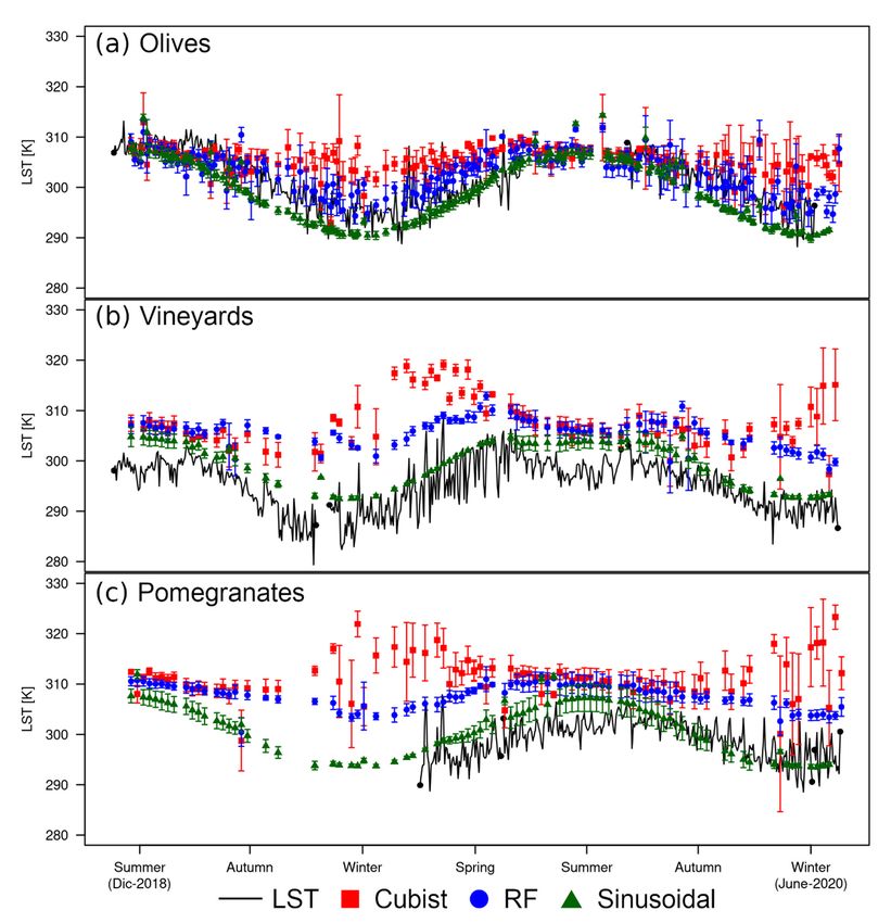
Remote Sens. 2021, 13, 4105                                                                                          2 of 21

                                   The actual evapotranspiration (ETa) is generally predicted as a fraction of maximum
                              evapotranspiration, which through an energy balance approach is calculated from remotely
                              sensed LST [7]. Furthermore, some methodologies integrate this LST approach in their ETa
                              estimation, such as the Operational Simplified Surface Energy Balance Model (SSEBop)
                              that relies on the LST, and the reference evapotranspiration (ETo) for ETa modeling [7–9].
                                   However, satellites have different sets of optical and thermal sensors, spatial reso-
                              lutions, and frequency of data acquisition. Usually, higher temporal resolution satellites
                              have lower spatial resolutions; therefore, combining and relating different satellite sensors
                              measurements is necessary in order to obtain higher frequencies and resolutions in areas
                              with contrasting land surfaces. The development of disaggregation of remotely sensed
                              LST (DLST) [10] allows for the capture of greater spatial differences in LST, which become
                              valuable in semiarid ecosystems with bare soil and vegetation variability at short dis-
                              tances [11]. The DLST methodologies can be used in surface energy balance models for ETa
                              modeling at higher spatial resolutions [12]. Currently, machine learning algorithms, such
                              as cubist (Cub) [13,14] and random forests (RF) [15], have been evaluated in downscaling
                              LST, but not in semi-arid ecosystems. Linear models [16,17], algorithms of RF [18–21]
                              and cubist [19,20], have been used successfully for DLST, arguing that the use of machine
                              learning approaches in capturing non-linear outliers is less sensitive than using linear
                              functions [22].
                                   The ET applications of DLST has been used in monitoring crop water requirements
                              during the growing season [23]. However, ET quantification using remote sensing monitor-
                              ing might get affected by the abovementioned differences between highly contrasting areas
                              with cultivated, low vegetation density, such as a desert [11]. The semi-arid ecosystem of
                              the Atacama Desert is characterized by a lack of precipitation, low humidity, and low cloud
                              coverage [24–26]. Furthermore, in the Copiapó valley, several water-demanding activities
                              coexist, increasing the stress in water use and decreasing water availability [27]. These
                              practices contribute to increased pressure over water use in the valley, and a clear analysis
                              of the water balance should be considered when evaluating the sustainable use of water,
                              food security, and decision making [28]. Therefore, looking for higher frequency estimation
                              of ET by remote sensing at a higher resolution provided by Sentinel-2 images might be a
                              proficient alternative to water assessment in an area where water conflicts may arise. The
                              aims of this study were (i) to downscale LST from optical sensor and indices derived from
                              Sentinel-2 at 10 m using observations from the Thermal Infrared Sensor (TIRS) of Landsat-8
                              using cubist, RF, and a sinusoidal model; and (ii) to estimate ETa using the DLST approach
                              applied in the SSEBop model in an arid or semi-arid climate of the Copiapó valley.

                              2. Materials and Methods
                              2.1. Study Area
                                   The area of study is in the Copiapó valley in the Atacama Region, Chile. The Copiapó
                              river watershed is about 18,538 km2 , stretching from the Andes to the Pacific Ocean coast.
                              The area of study is located in the nearest zone to the pacific coast (Figure 1). In this
                              section of the valley, the water source is mainly from aquifers, extracted through wells
                              and applied with high-frequency irrigation systems [29] (Figure 1). The agriculture in this
                              sector is dominated by olive trees, table grape orchards, pomegranates, tomatoes, and
                              natural vegetation. The climate is semiarid to arid, with hot and dry summer seasons, and
                              28 mm of mean annual precipitation [27,30].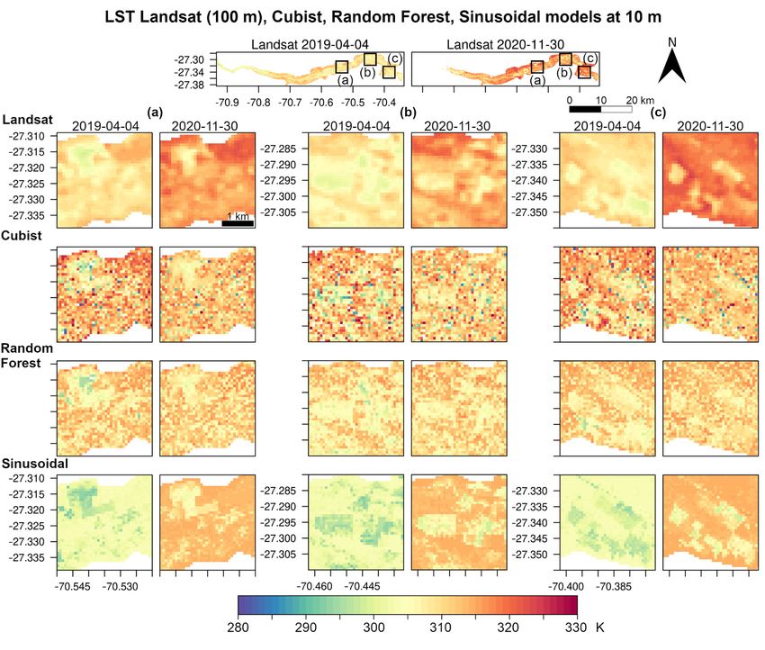
Remote Sens. 2021, 13, 4105 3 of 21
Remote Sens. 2021, 13, x FOR PEER REVIEW 3 of 22
Figure 1. Study area delimited by a green light dashed line (top). Location of three meteorological stations distributed in
Figure 1. Study area delimited by a green light dashed line (top). Location of three meteorological stations distributed in
olives (green circle), vineyards (red diamond), and pomegranates (blue triangle).
olives (green circle), vineyards (red diamond), and pomegranates (blue triangle).
2.2. Local Data
2.2. Local Data
Meteorological stations data were obtained from LAB-network [31], located across
Meteorological stations data were obtained from LAB-network [31], located across
the valley over three crops, as was described in Mattar et al. [31] and Olivera-Guerra et al.
the valley over three crops, as was described in Mattar et al. [31] and Olivera-Guerra
[27]. Crop coefficients (kc) used are in concordance with those used by Olivera-Guerra et
et al. [27]. Crop coefficients (kc) used are in concordance with those used by Olivera-Guerra
al. [27]
et al. forfor
[27] olives and
olives andvineyards
vineyards (Table
(Table1),
1),and
andthethepomegranates
pomegranateskckcvalues
values were
were adapted
adapted
from
from Franck [32] and Otárola Aliaga [33], which estimated kc values to arid and
Franck [32] and Otárola Aliaga [33], which estimated kc values to arid and semiarid
semiarid
conditions
conditions in in Chile.
Chile. The
The stations
stations located
located in
in olives
olives and
and vineyard
vineyard orchards
orchards have
have aa continuity
continuity
of in situ data from January 2016, while the pomegranates station started
of in situ data from January 2016, while the pomegranates station started to measure to measure in
in the
the winter
winter of 2019,
of 2019, all orchards
all orchards are under
are under dripdrip irrigation.
irrigation.
Table 1. Olives,
Table 1. Olives, vineyards,
vineyards, and
and pomegranates
pomegranates kc
kc values.
values.
Crop
Crop
Jan Jan
FebFeb Mar Mar
Apr May Jun
Apr May Jun
Jul
Jul
Aug
Aug
Sep
Sep
Oct
Oct
Nov Dec
Nov
Dec References
References
Olives 0.65 0.65 0.65 0.65 0.6 0.5 0.5 0.5 0.6 0.6 0.65 0.65 [27]
Olives 0.65 0.65 0.65 0.65 0.6 0.5 0.5 0.5 0.6 0.6 0.65 0.65 [27]
Vineyards
Vineyards 0.7 0.70.650.65 0.60.6 0.50.5 0.40.4 0.40.4 0.4
0.4 0.4
0.4 0.4
0.4 0.6
0.6 0.65
0.65 0.70.7 [27]
[27]
Pomegranates
Pomegranates 0.6 0.60.680.68 0.80.8 0.45
0.45 0.40.4 0.115
0.115 0.115
0.115 0.3
0.3 0.3
0.3 0.4
0.4 0.4 0.45
0.4 0.45 [32,33]
[32,33]
2.3. Remote Sensing Data
2.3. Remote Sensing Data
The product used for remote sensing was the Level 1-C Top of Atmosphere Reflec-
The product used for remote sensing was the Level 1-C Top of Atmosphere Reflectance
tance (TOA) and Surface Reflectance from Landsat 8 Level 2-A product. Thermal data
(TOA) and Surface Reflectance from Landsat 8 Level 2-A product. Thermal data were
were obtained from band 10 digital numbers (ND) of Landsat 8 Thermal Infrared Sensor
obtained from band 10 digital numbers (ND) of Landsat 8 Thermal Infrared Sensor (TIRS)
(TIRS) for the 2016–2020 period. Landsat-8 and Sentinel-2 images were cloud masked us-
for the 2016–2020 period. Landsat-8 and Sentinel-2 images were cloud masked using the
ing the Fmask 4.0 algorithm [34], and spatially matched according to the study area and
Fmask 4.0 algorithm [34], and spatially matched according to the study area and study
study period. There were 27 dates that match between Landsat-8, and Sentinel-2 used for
model calibration and validation. For each match date of Sentinel-2 and Landsat-8 TIRS
Remote Sens. 2021, 13, 4105                                                                                        4 of 21

                              period. There were 27 dates that match between Landsat-8, and Sentinel-2 used for model
                              calibration and validation. For each match date of Sentinel-2 and Landsat-8 TIRS images,
                              18 pairs of images were used in calibration of the Cub, RF, and sinusoidal (Sin) models,
                              and 9 pairs of images for validation of the LST were estimated.

                              2.4. Methodology
                              2.4.1. Surface Reflectance Retrieval
                                   The Sentinel 2 Level 2-A Surface Reflectance product was retrieved using a sen2cor
                              processor [35], which corrects the image using Water Vapour (WV) and Aerosol Optical
                              Thickness (AOT). This method performs atmospheric correction using Look-Up tables
                              from libRadtran [36] using as baseline the mid-latitude summer (MS) for the aerosol and
                              water vapour concentration for the study area. Water Vapour is obtained with Atmosphere
                              Pre-Corrected Differential Absorption algorithms [37] using the B8A and B9 bands for
                              reference channels in the atmospheric window and absorption region, respectively. The
                              Aerosol Optical Thickness is derived from 550 nm using the Dense Dark Vegetation (DDV)
                              algorithm [38], which correlates B12 versus VIS (B2, B3, B4). In order to determine the
                              impact atmospheric inputs of the imagery, we assessed the mean value, standard deviation
                              and coefficient of variation (cv) per pixel of WV and AOT for the study period. We
                              evaluated the impact of topographic illumination relating the hillshade of every image
                              versus the bands and NDVI determining the coefficient of determination of the imagery.

                              2.4.2. Land Surface Temperature Retrieval
                                   The Landsat-8 LST was determined by a single-channel algorithm using the band
                              10 [39], which is defined as

                                                                  1
                                                         LST = γ (ϕ1 ·Lsen + ϕ2 ) + ϕ3 + δ                    (1)
                                                                  ε

                              where γ, δ are two parameters that depend on the at-sensor brightness temperature, ε is
                              surface emissivity, and ϕ1 , ϕ2 , ϕ3 are the atmospheric functions versus atmospheric water
                              vapor content [40,41]. These input data of the atmospheric functions were obtained by
                              polynomial equations proposed by Cristóbal et al. [40] using NCEP/NCAR Reanalysis
                              data, which models the ascending, descending, and ascending atmospheric radiance and
                              transmittance (Lup, Ldown, and T, respectively). The ε input was obtained from the ASTER
                              Global Emissivity Dataset (ASTER GED) [42]. Thermal radiance (Lsen) was obtained from
                              radiometric calibration of band 10. This LST obtained from Landsat-8 will be used as the
                              observed data, and Sentinel-2 bands and spectral indices were considered as predictors for
                              the LST modeling.

                              2.4.3. Predictors
                                    The dataset used as predictors were 13 bands from Sentinel-2 plus 22 remote sensing
                              indices (Table 2), which were used as calibration data for the Cub and RF methods. The
                              pixel resolution for Landsat-8 LST and NDVI was 100 m as the observation data, and 10 m
                              for the Sentinel-2 bands and indexes. Sentinel-2 data were resampled to 100 m at each date
                              for modeling as predictors at 100 m and 10 m. The range of images acquisition was from
                              February 2016 to January 2019 in the calibration data, and from April 2019 to April 2020 in
                              the validation data in the matching dates, and Sentinel-2 data between February 2016 and
                              June 2020.
Remote Sens. 2021, 13, 4105 5 of 21
Table 2. Set of sentinel bands and indexes tested for LST modeling.
Name Variables Sentinel-2 Variables Expression References
B1 Band 1
B2 Band 2
B3 Band 3
B4 Band 4
B5 Band 5
B6 Band 6
B7 Band 7
B8 Band 8
B8A Band 8A
B9 Band 9
B11 Band 11
B12 Band 12
NIR−Red
NDVI Normalized difference vegetation index NIR+Red [43]
NIR−Red
SAVI Soil adjusted vegetation index NIR+Red+L × (1 + L) [44]
NIR−Red
EVI Enhanced vegetation index G × NIR+C1 ×Red−C2×+L [45]
NIR−Green
GNDVI Green normalized difference vegetation index NIR+Green [46]
Green−NIR
NDWI Normalized difference water index [47]
q Green+NIR
2
2·NIR+1− (2·NIR+1) −8·(NIR−Red)
MSAVI2 Modified soil vegetation index 2 [48]
2
ALBEDO Albedo α = ∑B i |ρB i ·ωB i | [49]
B8a−B5
SELI Sentinel-2 LAIgreen index B8a+B5 [50]
TCARI Transformed chlorophyll absorption ratio index 3·((B5 − B4) − 0.2·(B5 − B3)(B5/B4)) [51]
(1+0.16)(NIR−Red)
OSAVI Optimized soil adjusted vegetation index NIR+Red+0.16 [52]
TCARI
TCARI/OSAVI OSAVI [51,52]
Green−Red
GRVI Green-Red vegetation index Green+Red [53]
0.1·NIR−Red
WDRVI Wide dynamic range vegetation index 0.1·NIR+Red [54]
0.1·NIR−Blue
BWDRVI Blue-wide dynamic range vegetation index 0.1·NIR+Blue [55]
√
TVI Transformed vegetation index NDVI + 0.5 [43]
NIR−Red−y(Red−Blue)
ARVI Atmospherically resistant vegetation index NIR+Red−y(Red−Blue)
[56]
B8−B1
SIPI Structure insensitive pigment index B8−B4 [57]
(SWIR+Red)−(NIR+Blue)
BSI Bare soil index (SWIR+Red)+(NIR+Blue)
[58]
B11
MSI Sentinel-2 Moisture stress index B8 [59]
B9
GCI Green chlorophyll index B3 − 1 [60]
NIR−SWIR
NDMI Normalized difference moisture index NIR+SWIR [61]
B9
CLRE Red-edge-band Chlorophyll Index B5 − 1 [60]
G, C1, C2: Coefficients; NIR: Near infrared; SWIR: short wave infrared; ρBi : surface reflectance at band Bi; ωBi : weighting coefficient at
band Bi.
2.4.4. Spatial Relationship between Landsat-8 LST and Sentinel-2
The spatial relationship between Landsat-8 LST and predictors from Sentinel-2 were
by two machine learning algorithms, cubist [13,14] and random forests [15,62], and one
through a sinusoidal relationship between LST and NDVI [27], based on Bechtel et al. [16]
and Bechtel [63,64]. For building each model, the LST at 100 m is the target variable,
excepting NDVI at 100 m, which is also needed for the sinusoidal model. The Sentinel-2
Remote Sens. 2021, 13, 4105                                                                                          6 of 21

                              images at 100 m are used to predict LST at 100 m according to each model; later, each
                              Sentinel-2 at 100 m calibrated model was used to predict LST using 10 m Sentinel-2
                              predictors.
                                    A cubist model is a tree of rules limited by conditions based on values or ranges of
                              predictors. Each rule has a linear model that predicts the target value of a pixel in that
                              condition. In this approach, the 27 calibration dates were spatially matched using the
                              whole set of predictors using the Cubist package [65] in R open source software [66].
                                    A random forest model consists of many decision trees that use several random
                              subsampling creating a learning model based on classification or regression trees. The
                              same 27 calibration dates of Sentinel-2 images were applied for prediction targeting LST
                              from Landsat-8 with the randomForest package [67,68]. Furthermore, the variable selection
                              for random forest algorithm (VSURF) was applied to allow parsimony and evaluate which
                              predictors performed better predicting LST with random forests. The VSURF algorithm
                              is implemented in R software by Genuer et al. [69,70]. Due to its high computational
                              demand, the algorithm was run in Wageningen University’s High Performance Computing
                              Cluster (HPC), Anunna. The process involved 25 random samples of 11,000 points from
                              the whole calibration dataset per each VSURF run. Then, 50 RF with 2000 trees each were
                              run at each sample, and then the results were ranked by variable importance averaging of
                              50 RF runs [69]. Later, VSURF has three outcomes of the selected variables: thresholding,
                              interpretation, and the prediction step. We chose interpretation, because it involves more
                              variables than a prediction step, and it reduces overfitting from the thresholding step.
                              Finally, the sum of the variables selected from those 25 VSURF runs were used as the set of
                              variables in the RF prediction.
                                    The sinusoidal modeling is based on a general linear relationship between LST and
                              NDVI [71]:
                                                                LST10m = a + b·NDVI10m                                (2)
                                   Furthermore, this relation is seasonal during the year, allowing estimation of annual
                              cycle parameters according to Bechtel et al. [16] and Bechtel [63,64]. The relationship
                              between LST and NDVI was validated for DLST in the study by Olivera-Guerra et al. [27].

                                                           LSTL8 100m = ci + di ·NDVIS2 100m                            (3)

                              where c is intercept and d is the slope from the fitted linear values of Landsat-8 LST and
                              Sentinel-2 NDVI at each i-calibration date. Therefore, the linear coefficients c and d can
                              be modeled as annual cycle parameters depending on the day of the year relative to the
                              spring equinox.
                                                                           DOY as equinox ·2π

                                                         c = e + f · sin                                              (4)
                                                                                 365
                                                                           DOY as equinox ·2π

                                                        d = g + h· sin                                                (5)
                                                                                  365
                              where c and d are linear coefficients of the LST–NDVI relationship to each image date. The
                              e, f, g, and h are fitted coefficients of the relationship between the day of the year with c
                              and d. The spring equinox is 21 September in the southern hemisphere, with a value of 0
                              to that day of DOY as equinox; therefore, −182.5 ≤ DOY as equinox ≤ 182.5. These c and d
                              coefficients from the calibration dates were used for estimating a and b from Equation (2)
                              using the fitted values of e, f, g, and h for a 10 m resolution.

                              2.4.5. Estimation of Actual Evapotranspiration
                                     The ET estimation method was the Operational Simplified Surface Energy Balance
                              (SSEBop) [9]. The SSEBop model has been widely applied at different hydroclimatic
                              regions [7], which is based on the estimation of the ET fraction (ETf), which is the ratio
                              of latent heat flux to the Net Radiation. The ETf is retrieved using surface temperature
                              (Ts ), cold/wet (Tc ), and hot/dry (TH ) idealized surface temperature conditions from
Remote Sens. 2021, 13, 4105                                                                                            7 of 21

                              Bastiaanssen et al. [72]. Thus, ETf is calculated using the following equations from Senay
                              et al. [9]:
                                                                       T − Ts     T − Ts
                                                               ETf = H          = H                                   (6)
                                                                       TH − Tc       dT
                                                                             Rn ·rah
                                                                      dT =                                                (7)
                                                                             ρa ·Cp
                              where dT is the difference in surface temperature between the idealized conditions and is
                              calculated under clear-sky conditions and is unique for location and day of the year (DOY),
                              but with the assumption of not changing from year to year [8]. rah is the aerodynamic
                              resistance to heat in an idealized bare and dry surface (s m−1 ), which was used the value of
                              110 sm−1 from Senay et al. [9]; ρa is the air density estimated by a function of air pressure
                              and the virtual temperature (Tkv ) [73]. Cp is the specific heat at a constant air pressure
                              (1.013 kJ kg−1 K−1 ). TH is calculated by TH = Tc + dT, and Tc is calculated by the relation of
                              the maximum air temperature and a correction factor of 0.093 (Tc = 0.093 Tmax ) [9,27]. The
                              Rn is clear-sky net radiation (W m−2 ), and Rn was obtained calculating the ratio between
                              daily net radio and instantaneous radiation (Cdi ) in the function of DOY from Sobrino
                              et al. [74], adapted by Moletto-Lobos [75] to the southern hemisphere:

                                              DOY ≥ 183 ⇒ −7·10−6 (DOY − 183)2 + 0.0027(DOY − 183) + 0.124

                                  Cdi =                                                                                   (8)
                                              DOY < 183 ⇒ −7·10−6 (DOY + 183)2 + 0.0027( DOY + 183) + 0.124

                                   Then ETf is calculated using the Ts derived from the downscaled LST of Cub, RF,
                              and Sin method. ETa is calculated using ETf, the maximum crop coefficient (kc) during
                              the phenological season by an aerodynamically rougher crop of 0.65 according to Olivera-
                              Guerra et al. [27,76], and the calculated evapotranspiration of reference (ETo) using the
                              standardized Penman–Monteith equation [73,77]:

                                                                 ETa = ETf × kc × ETo                                     (9)

                                    The ETo was calculated using the atmospheric inputs from the ERA5 product [78].
                              In previous studies using the SSEBop model by Senay et al. [8], they have defined those
                              negative values of ETf are set to zero and maximum ETf are capped at 1.05. According to
                              Senay et al. [7], ETf should vary between 0 and 1; therefore, in this study negative ETf were
                              set to zero and capped to 1.

                              2.4.6. Validation In Situ
                                   The validation of the downscaled LST and measured Landsat-8 LST were with the in
                              situ LAB-net stations, and their thermal infrared sensor (Apogee SI-111® ). This sensor is
                              located at 5 m height with the inclination to measure the same fraction of vegetation cover
                              of the terrain. The values of LST were extracted from the downscaled images to compare
                              them with in situ stations. The in situ value were obtained by the mean of the surrounded
                              pixels at the position of the corresponding olive, vineyard, and pomegranate stations. For
                              the comparison of in situ ET, the crop evapotranspiration (ETc) was calculated using the
                              ET calculated by the weather station and multiplying the monthly corresponding kc of
                              each crop (ETc = ETo ·kc), following the coefficients shown in Table 1. The performance
                              metrics were the root mean square error (RMSE), standard deviation (sigma), bias, and
                              correlation coefficient (r) for the nine LST validation dates that match between Landsat-8
                              and Sentinel-2.

                              3. Results
                              3.1. Atmospheric Inputs and Topographic Variation
                                   The atmospheric inputs of Sentinel 2 correction are shown in Supplementary Figure S1
                              for AOT. The mean value shows values related to clear sky places, such as the Atacama
                              Desert, with a mean value of 0.17 and standard deviation of 0.01, without variability over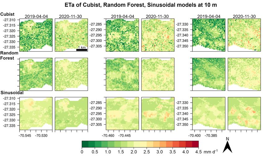
Remote Sens. 2021, 13, 4105                                                                                            8 of 21

                              the time series. The WV (Supplementary Figure S2) had a mean value of 1.13 cm and
                              coefficient of variation of 13.4%. The atmospheric inputs show an artifact due to the method
                              of calculation on the center of study area; however, the low values of atmospheric water
                              vapor do not change over values of an atmospheric profile for a semi-arid ecosystem. On
                              the other hand, the coefficient of determination of hillshade of every image versus the
                              input bands does not show any relation due to the flat terrain in the study area, with an
                              average slope of 3%. The part that reaches the highest correlation is in the red band with
                              an R2 of 0.2 in the place steeper area of 41%.
                                    The atmospheric inputs of Landsat 8 are in Supplementary Table S1, where Ldown
                              shows the most variation, with a maximum value of 5.70 W m−2 sr−1 , minimum of
                              1.29 W m−2 sr−1 , and coefficient of variation up to 28.41%. The Lup showed lower vari-
                              ability, with a cv of 16.06% and transmittance with cv of 9.42% and mean of 0.77 for the
                              study period.

                              3.2. Cubist
                                   The Cub output created a hundred rules for predicting LST, showing that almost all
                              the predictors are used for prediction, but not all of them in defining the set of rules of the
                              trees (Figure 2A). The most used variables in the algorithm to separate the conditions were
                              B9 (all conditions) and then B11 and TCARI, participating in 63% and 53% of the rules,
                              respectively.

                              3.3. Random Forest
                                   The results of the VSURF algorithm (Figure 2B) show that in the 25 runs in the HPC
                              computer, the variables selected for model interpretation after running 50 RF with 2000
                              trees per HPC run are B9, B11, B12, and TCARIOSAVI, which were selected in all VSURF
                              runs, secondary CLRE in 23, and B1 in 20. The other variables were selected in a minor
                              proportion but were included in the set of predictors used in the RF spatial prediction of
                              LST at 100 m. Therefore, the RF model parsimony from VSURF that was used in the RF
                              prediction of LST resulted in a total of 11 variables (Figure 2B,C). The variable importance
                              as a percentage of increase in MSE, when one of these variables is out of the model, shows
                              that the most important variables are B9, TCARIOSAVI, CLRE, and B1 (Figure 2C).

                              3.4. Sinusoidal
                                   The sinusoidal model and observed fitted values according to the day of year relative
                              to the spring equinox are shown in the Figure 2D,E, resulting in an intercept and slope
                              modeling equation c and d of

                                                                              DOY as equinox ·2π

                                                   c = 306.148 + 9.977· sin                                         (10)
                                                                                    365

                                                                              DOY as equinox ·2π

                                                  d = −14.118 − 5.047· sin                                          (11)
                                                                                     365
                                    The validation results (Figure 3) showed that for 100 m, the RMSE values were 5.77 K
                              for Cub, 4.81 K for RF, 3.97 K for Sin models, and 6.4 K of Landsat-8 at 100 m. In terms of
                              variation, the values of sigma followed the same previous trend with Cub with the higher
                              values, followed by RF and then Sin. The RF and Cub models slightly overestimate and
                              Sin underestimates LST, but also the correlation coefficient is the lowest for RF, followed by
                              Cub and Sin with the best performance. In the 10 m prediction model, the trend in RMSE
                              is similar: Cub performed with the highest RMSE 7.09 K, RF with 3.91 K, and 3.4 K for Sin.
                              Besides, Cub shows a higher variation and overestimation of LST compared to the in situ
                              values. RF at 10 m has a higher correlation coefficient and lower RMSE compared with
                              100 m. The Sin model shows an underestimation, the highest correlation coefficient, and
                              lowest variation in the two-resolution LST estimation compared to in situ.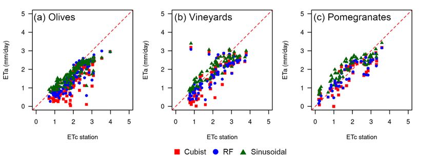
Remote Sens. 2021, 13, 4105                                                                                                                     9 of 21
            Remote Sens. 2021, 13, x FOR PEER REVIEW                                                                                 9 of 22

         Remote Sens. 2021, 13, x FOR PEER REVIEW                                                                                       10 of 22

                                            K for Sin. Besides, Cub shows a higher variation and overestimation of LST compared to
                                            the in situ values. RF at 10 m has a higher correlation coefficient and lower RMSE com-
                 Cubist2.(A),
      Figure 2. Figure         variable
                           Cubist           pared
                                          selection
                                  (A), variable     with
                                                selection  100random
                                                      for for  m. The
                                                          random       Sin algorithm
                                                                   forest
                                                                     forest model   shows
                                                                            algorithm       an underestimation,
                                                                                       (B),random
                                                                                      (B),   random  forest
                                                                                                  forest (C), (C), the highest
                                                                                                                   and          correlation
                                                                                                                       sinusoidal
                                                                                                              and sinusoidal (D,E)          coef-
                                                                                                                                    (D,E) model
                                                                                                                                   model
      calibrationcalibration
                   results. results.        ficient, and lowest variation in the two-resolution LST estimation compared to in situ.

                                                  The validation results (Figure 3) showed that for 100 m, the RMSE values were 5.77
                                             K for Cub, 4.81 K for RF, 3.97 K for Sin models, and 6.4 K of Landsat-8 at 100 m. In terms
                                             of variation, the values of sigma followed the same previous trend with Cub with the
                                             higher values, followed by RF and then Sin. The RF and Cub models slightly overestimate
                                             and Sin underestimates LST, but also the correlation coefficient is the lowest for RF, fol-
                                             lowed by Cub and Sin with the best performance. In the 10 m prediction model, the trend
                                             in RMSE is similar: Cub performed with the highest RMSE 7.09 K, RF with 3.91 K, and 3.4

      Figure 3.  Validation
              Figure         resultsresults
                      3. Validation   of the of
                                             predicted   LST with
                                                the predicted     cubist,
                                                              LST with    random
                                                                       cubist,      forest,
                                                                               random       and
                                                                                       forest,   sinusoidal
                                                                                               and sinusoidalmodels
                                                                                                              modelsversus
                                                                                                                     versus the
                                                                                                                            the LST measured
                                                                                                                                LST meas-
              ured
      by in situ    by in situ stations.
                 stations.

                                                  The models are applied in a temporal series of LST at 100 m and 10 m (Figures 4 and
                                            5, respectively) after validation dates in each crop, showing a general trend according to
                                            the bias validation results (Figure 3). For olives, the LST in all models is very similar to the
                                            LST trend during the seasons. However, Cub and RF overestimates the LST values of the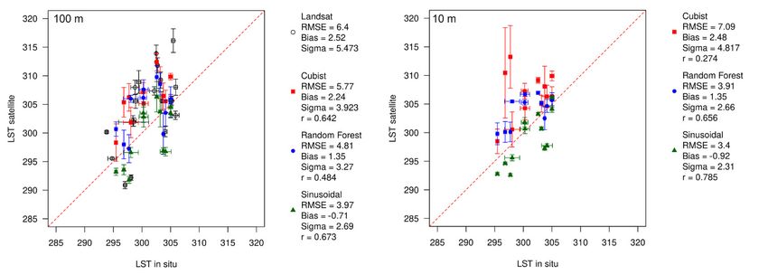
Remote Sens. 2021, 13, 4105                                                                                                    10 of 21

                                          The models are applied in a temporal series of LST at 100 m and 10 m (Figures 4 and 5,
                                    respectively) after validation dates in each crop, showing a general trend according to the
                                    bias validation results (Figure 3). For olives, the LST in all models is very similar to the
                                    LST trend during the seasons. However, Cub and RF overestimates the LST values of the
                                    station in winter and estimating in an opposite trend to the seasonal LST decrease in winter.
                                    The Sin model shows a tendency of seasonal variation of LST with a slight underestimation
                                    of LST, similar to bias validation results in Figure 3. In vineyards, the standard deviation of
                                    the surrounding pixels at the station of LST in Cub are higher than the other models and
                                    showed an increase in the winter LST estimated. The main difference in the 10 m resolution
Remote Sens. 2021, 13, x FOR PEER REVIEW                                                                                   11 of 22
                                    (Figure 5) is that Cub evidently has a higher standard deviation and is overestimating LST
                                    compared to the station in winter.

      Figure 4. Temporal series of the predicted Sentinel-2 LST at 100 m of the cubist, random forest, and sinusoidal models
      compared to the LST measured by the in situ stations at (a) olives, (b) vineyards,
                                                                              vineyards, and (c) pomegranates
                                                                                                 pomegranates orchards. The error
      bars are showing the standard  deviation of the 9 pixel cells surrounding  the LST  station
      bars are showing the standard deviation of the 9 pixel cells surrounding the LST station of of each
                                                                                                     each LST
                                                                                                          LST model.
                                                                                                              model.
Remote Sens. 2021, 13, 4105 11 of 21
Remote Sens. 2021, 13, x FOR PEER REVIEW 12 of 22
Figure 5.
5. Temporal
Temporalseries
seriesofofthe
the predicted
predicted Sentinel-2
Sentinel-2 LSTLST atm
at 10 10ofmthe
ofcubist,
the cubist,
randomrandom
forest,forest, and sinusoidal
and sinusoidal modelsmodels
versus
versus
the LSTthe LST measured
measured by the by
in the
situin situ stations
stations at (a) at (a) olives,
olives, (b) vineyards,
(b) vineyards, and
and (c) (c) pomegranates
pomegranates orchards.
orchards. The The
errorerror
barsbars
are
are showing
showing the the standard
standard deviation
deviation of 9the
of the 9 pixel
pixel cellscells surrounding
surrounding the LST
the LST station
station of each
of each LST LST model.
model.
The
The spatial
spatial prediction images (Figure 6) showed that in winter LST is higher for Cub
and
and RF
RF and
and lower
lower for Sin at a 10 m resolution. Warmer pixels next to vegetation can be
attributed
attributed toto be
be bare soil captured by Landsat-8, which are colder in the Sin model. The
Cub model shows aahigh
Cub model shows highvariation
variationinin predicted
predicted LST LST pixels
pixels in ainshort
a short range
range of spatial
of spatial var-
variation.
iation. Pixels
Pixels varied
varied between
between 280280
to to
290290
KK nexttotothe
next thewarmest
warmestwithout
withoutaaspatial
spatial relation
relation
to vegetation according
to accordingto toLandsat-8.
Landsat-8.In Insummer,
summer,allallmodels
models showed
showed spatially colder
spatially values
colder val-
thanthan
ues Landsat-8. The Sin
Landsat-8. Themodel showsshows
Sin model a clearadistinction between
clear distinction vegetation
between areas, and
vegetation RF
areas,
doesRF
and notdoes
show nota show
clear spatial
a clear trend
spatialwith vegetation,
trend but thebut
with vegetation, coldest pixels are
the coldest related
pixels to
are re-
areas with vegetation.
lated to areas with vegetation.
After being applied, the ETa spatial prediction of olives, vineyards, and pomegran-
ates at 10 m were generated (Figure 7). The results showed winter (left) and a summer
(right) images to each model of ETa per day, Cub and RF showed lower values of ETaWhen the ETa temporal series is analyzed at 100 m (Figure 8) and 10 m (Figure 9),
the values estimated for olives match almost entirely with ETc from the stations and kc
values defined in Table 1. The Cub model shows an underestimation in winter, but all the
other models followed the ETc seasonal variation in situ with an underestimation in sum-
Remote Sens. 2021, 13, 4105 mer. For pomegranates, the trend is the opposite, where generally all the models overes-
12 of 21
timate the ETc of station from winter to summer; however, in late 2019 summer to 2020
autumn, the estimated ETa followed the same trend as the station.
Figure 6. Land
Figure 6. Land surface
surface temperature
temperature byby Landsat-8
Landsat-8 atat 100
100 m
m and
and the
the spatial
spatial predictions
predictions of
of LST
LST from
from Sentinel-2
Sentinel-2 data
data using
using
cubist, random forest, and sinusoidal models.
cubist, random forest, and sinusoidal models. The predictions are shown at two dates apr 04 2019 (winter) and nov 11 2020
(late spring) in three locations next to the olives (a), vineyards (b), and pomegranates (c) stations.
After being applied, the ETa spatial prediction of olives, vineyards, and pomegranates
at 10 m were generated (Figure 7). The results showed winter (left) and a summer (right)
images to each model of ETa per day, Cub and RF showed lower values of ETa compared
to Sin in winter, and summer images are spatially similar in values with a clear distinction
of crops by Sin. Although, with abrupt changes in closer pixels for Cub. In vineyards,
a distinction is clear in winter for Sin, with higher values of ETa in the valley compared
to Cub and RF. In the summer, the condition of short-range variation in ETa values in
Cub continued similar to what was observed in the LST prediction, and RF and Sin also
performed similarly. Pomegranate spatial values show a distinction of Sin in winter,
showing higher values of ETa in the entire valley compared with Cub and RF. In the
summer it performed similarly, but Cub continuously showed abrupt changes in a short
range of pixels.Remote
Remote Sens.Sens. 13, x13,FOR
2021,2021, 4105PEER REVIEW 13 of 2114 of 22
Figure
Figure 7. ETa
7. ETa based
based onon Kmaxatat10
Kmax 10m
mestimated
estimated from
fromDLST
DLSTwith
withcubist, random
cubist, forest,
random and sinusoidal
forest, models.
and sinusoidal models.
When the ETa temporal series is analyzed at 100 m (Figure 8) and 10 m (Figure 9), the
values estimated for olives match almost entirely with ETc from the stations and kc values
defined in Table 1. The Cub model shows an underestimation in winter, but all the other
models followed the ETc seasonal variation in situ with an underestimation in summer.
For pomegranates, the trend is the opposite, where generally all the models overestimate
the ETc of station from winter to summer; however, in late 2019 summer to 2020 autumn,
the estimated ETa followed the same trend as the station.Remote Sens.
Remote 2021,
Sens. 13,13,
2021, x FOR
4105PEER REVIEW 1415
of of
21 22
Figure
Figure 8. Temporal
8. Temporal series
series ofof
thethe predictedETa
predicted ETaatat100
100mmwith
with cubist,
cubist, random
random forest,
forest,and
andsinusoidal
sinusoidalmodels
models versus thethe
versus ETa
ETa
measured
measured byby
thethe
ininsitu
situstations
stationsatat (a)
(a) olives,
olives, (b)
(b)vineyards,
vineyards,and
and(c)(c)
pomegranates orchards.
pomegranates The The
orchards. errorerror
bars are
barsshowing the
are showing
thestandard
standarddeviation
deviationofof the
the 9 pixel
9 pixel cells
cells surrounding
surrounding the the
ETc ETc station
station of each
of each ETa model.
ETa model.Remote Sens.
Remote 2021,
Sens. 13,13,
2021, x FOR
4105 PEER REVIEW 1516 of 22
of 21
Figure 9. Temporal
Figure 9. Temporalseries
seriesofofthe
the predicted ETaatat1010mmwith
predicted ETa with
thethe cubist,
cubist, random
random forest,
forest, and sinusoidal
and sinusoidal models
models versusversus
the ETathe
ETameasured
measured by the in situ stations at (a) olives, (b) vineyards, and (c) pomegranates orchards. The error bars are
by the in situ stations at (a) olives, (b) vineyards, and (c) pomegranates orchards. The error bars are showing showing
the
thestandard
standarddeviation
deviation of the 9 pixel cells surrounding the ETc station of each ETa
of the 9 pixel cells surrounding the ETc station of each ETa model. model.
4.4.Discussion
Discussion
Testingand
Testing andcomparing
comparing new methods
methods that
thatquantify
quantifyETETfrom
fromirrigation
irrigationcrops is vital
crops is vital
ininareas
areaswith
withwater
waterscarcity,
scarcity, and detailed
detailedprediction
predictionmaps
mapsallow
allowa better
a betterdecision-making
decision-making
processamong
process amongwater
water users
users [4].
[4]. The
The model
model applied
appliedfor
forDLST
DLSTininETaETabased
basedononKmax
Kmaxareare
different spatially (Figure 7) and temporally (Figures 8 and 9), but the strength showed
different spatially (Figure 7) and temporally (Figures 8 and 9), but the strength showed by by
the SSEBop ET model is consistent (Table 3), making these differences in LST
the SSEBop ET model is consistent (Table 3), making these differences in LST predicted predicted
bybyeach
each model (Figures 4–6) lower between Cub, RF, and Sin in ETa compared to ETc
model (Figures 4–6) lower between Cub, RF, and Sin in ETa compared to ETc
(Figure 10). The best model overall predicting ETa analyzed over ETc was RF with an 2
(Figure 10). The best model overall predicting ETa analyzed over ETc was RF with an R
R2 = 0.710, Sin with 0.707, and an R2 of 0.69 for Cub. However, the Sin model was with
= 0.710, Sin with 0.707, and an R2 of 0.69 for Cub. However, the Sin model was with the
lowest RMSE of 0.45 mm d-1, smallest bias, standard deviation, relative root mean square
error (RRMSE), and mean absolute error. Besides, the Sin model is the best in olives and
vineyards in all statistical indices, with the highest R2 in all stations, but with the highestRemote Sens. 2021, 13, 4105 16 of 21
the lowest RMSE of 0.45 mm d−1 , smallest bias, standard deviation, relative root mean
square error (RRMSE), and mean absolute error. Besides, the Sin model is the best in olives
and vineyards in all statistical indices, with the highest R2 in all stations, but with the
highest RMSE in pomegranates. The Cub model showed the lowest performance in all
stations and overall analysis. This low ETa performance of Cub was noticed in the spatial
ETa (Figure 7), with high variation of pixels over a short distance range. The performance
of RF and Sin are consistent and similar in ETa at 10 m; nevertheless, there is a practical
advantage of using the Sin model based in NDVI calibration compared with the RF model
that is dependent on predictors to build a model by an empirical relation in one spatial
area only. The meta-analysis obtained from the machine learning algorithms also gave
approximations of a general approach estimating ET, which are evidenced by variables
related with LST that showed high importance in the algorithms and may be important
for improving future indices, equations, and models for calculating ET. However, the
performance of the Sin model and its calibration process showed that it might be easier
to apply with Sentinel-2 NDVI and without several calibration parameters that might be
needed or differ for an RF model in a different region.
Table 3. Model performance statistics of ETa estimated using cubist, random forest, and sinusoidal
models compared with the ETc over olives, vineyards, and pomegranates orchards.
ETa Cubist Random Forest Sinusoidal
Olives RMSE 0.75 0.56 0.39
Bias −0.35 −0.25 −0.12
Sigma 0.56 0.42 0.29
R2 0.673 0.750 0.798
RRMSE 29.21 16.52 7.85
MAE 0.62 0.46 0.26
Vineyards RMSE 0.72 0.62 0.49
Bias −0.15 −0.12 0.00
Sigma 0.42 0.36 0.29
R2 0.651 0.675 0.692
RRMSE 26.01 19.66 12.26
MAE 0.59 0.50 0.33
Pomegranates RMSE 0.48 0.44 0.50
Bias −0.03 −0.02 0.07
Sigma 0.25 0.23 0.26
R2 0.764 0.802 0.837
RRMSE 12.96 10.96 14.30
MAE 0.39 0.35 0.44
Overall RMSE 0.69 0.56 0.45
Bias −0.18 −0.13 −0.02
Sigma 0.43 0.35 0.28
R2 0.641 0.710 0.707
RRMSE 24.85 16.29 10.51
MAE 0.56 0.45 0.32cording to previous studies, the topographic effect can be reduced by band ratios, due to
the spectrum similarity between the NIR and visible bands [82,83]. About the limitations
of the approach, our study used non-supervised areas for calibration of the LST models,
using images of the whole study area instead of a selection of areas with vegetation, bare
soil, or other surfaces. Besides, the models were evaluated during the seasonal variation
Remote Sens. 2021, 13, 4105 17 of 21
of the agricultural vegetation; thus, they can perform differently in non-agricultural veg-
etation or in non-irrigated agriculture.
Figure Predicted
10. 10.
Figure PredictedETaETa
at the 10 m
at the 10 resolution of the
m resolution cubist,
of the random
cubist, forest,
random andand
forest, sinusoidal model
sinusoidal compared
model to the
compared ETcETc
to the
station in (a) olives, (b) vineyards, and (c) pomegranates.
station in (a) olives, (b) vineyards, and (c) pomegranates.
The SSEBop approach in arid ecosystems has been applied in quantification of irri-
gation in California [79], but it also might be a useful tool in ET estimations of semi-arid
agroecosystems, such as the Copiapó valley. According to Anderson et al. [4], ET methods
from vegetation indices tend to overestimate ET under stress conditions, showing higher
crop demands before biomass can adjust. However, an estimation based on vegetation
indices, such as the Sin method, might be useful as a primary approach in demand es-
timations in areas where water crop demand cannot be estimated using an ETc station
with kc by calendar, and used in other areas of the valley as well. Furthermore, a spa-
tial ET estimation based on Sentinel-2 frequency and spatial resolution would improve
water demand quantifications in semiarid ecosystems such as the Copiapó valley, where
groundwater demand is under pressure [29]. Monitoring these ecosystems will be crucial
in order to minimize and prevent future conflicts over water in arid and semiarid climates,
where higher water requirements will increase in the future [80,81]. It should be considered
that the topographic effect can bring noise to NDVI retrieval, especially for these areas.
According to previous studies, the topographic effect can be reduced by band ratios, due to
the spectrum similarity between the NIR and visible bands [82,83]. About the limitations of
the approach, our study used non-supervised areas for calibration of the LST models, using
images of the whole study area instead of a selection of areas with vegetation, bare soil, or
other surfaces. Besides, the models were evaluated during the seasonal variation of the
agricultural vegetation; thus, they can perform differently in non-agricultural vegetation
or in non-irrigated agriculture.
5. Conclusions
In this study, we evaluated three models to estimate and downscale LST using Sentinel-
2 images and remote sensing indices as predictors, comparing them with Landsat-8 LST
as the training data. The results of the LST predictions showed that the best model to
downscale LST was a sinusoidal model, which showed the lowest RMSE of 3.97 K at 100 m
and 3.4 K in 10 m, and with the highest correlation coefficients. The machine learning
analysis showed that the variable with the greatest importance in predicting LST was
Sentinel-2 band 9, as it was included in the majority of internal model conditions and
prediction rules. These models were applied in ETa estimation using the operational
surface energy balance method (SSEBop) with the downscaled LST, showing that the RF
and Sin models are useful in estimating ETa in a semi-arid region. On the contrary, the Cub
model was not reliable across space, not in the ETa predictions overall nor for the olives,
vineyards, and pomegranates compared to Sin and RF.
This approach shows an advantage of the Sin model, which relies on NDVI and an
equation related to the day of the year, and not on a set of other predictors. Therefore, a Sin
model approach makes it possible to predict LST using previous date matches of LandsatRemote Sens. 2021, 13, 4105 18 of 21
and Sentinel, without training a dataset that might vary between locations. The RF model
showed the best overall performance estimating ET compared to all ETc stations, but a Sin
model showed a similar performance to RF with the lowest RMSE in ETa in comparison to
ETc overall and in olives, vineyards, and pomegranates. Future research should focus on
improvements in Kc in situ measurements using ETa stations instead of Kc values from
calendar, also testing the model quantification in irrigation scheduling considering the soil
water content, saline stress, and plant ecophysiological variables.
Finally, this study contributes to estimating water demand in a semi-arid region by
providing ETa maps at higher temporal and spatial resolutions and are reliable for crop
water requirements and irrigation scheduling compared to ETc calculated with the kc
values from the calendar.
Supplementary Materials: The following are available online at https://www.mdpi.com/article/
10.3390/rs13204105/s1. Table S1. Statistics of Atmospheric inputs over Landsat 8 series. Figure S1.
Mean, Standard Deviation and Coefficient of Variation of Aerosol Optical Thickness (AOT) retrieved
from Sen2Cor for all images during study period over Copiapó valley. Figure S2. Mean, Standard
Deviation and Coefficient of Variation of Water Vapor (WV) retrieved from Sen2Cor for all images
during study period over Copiapó valley. Figure S3. Coefficient of determination (R2) between
Illumination and Sentinel 2 Bands, NDVI during study period in Copiapó valley.
Author Contributions: Conceptualization, L.A.R.R., I.M.-L., C.M., R.F. and C.E.-A.; Data curation,
L.A.R.R., I.M.-L., F.C., C.M. and R.F.; Formal analysis, L.A.R.R., I.M.-L., F.C. and C.E.-A.; Funding
acquisition, C.M., R.F. and C.E.-A.; Investigation, L.A.R.R., I.M.-L., F.C., C.M., R.F. and C.E.-A.;
Methodology, L.A.R.R., I.M.-L., F.C., C.M. and R.F.; Project administration, C.M., R.F. and C.E.-
A.; Resources, L.A.R.R., I.M.-L., F.C., C.M., R.F. and C.E.-A.; Software, L.A.R.R., I.M.-L. and F.C.;
Supervision, I.M.-L., C.M., R.F. and C.E.-A.; Validation, L.A.R.R., I.M.-L., F.C., C.M., R.F. and C.E.-
A.; Visualization, L.A.R.R. and F.C.; Writing–original draft, L.A.R.R.; Writing–review and editing,
L.A.R.R., I.M.-L., F.C., C.M., R.F. and C.E.-A. All authors have read and agreed to the published
version of the manuscript.
Funding: This work was funded by Chile’s National Agency of Research and Development (ANID)
[FONDEF project number IT18I0022].
Acknowledgments: We thank JWZ and SJV for proof reading the manuscript.
Conflicts of Interest: The authors have declared that no competing interest exist.
References
1. Fuster, R.; Moletto-Lobos, Í.G.; Mattar, C. Evapotranspiration monitoring. In Encyclopedia of Water: Science, Technology, and Society;
Maurice, P., Ed.; Wiley: Hoboken, NJ, USA, 2020; Volume 3, pp. 1327–1358. ISBN 978-1-119-30075-5.
2. Fisher, J.B.; Melton, F.; Middleton, E.; Hain, C.; Anderson, M.; Allen, R.; McCabe, M.F.; Hook, S.; Baldocchi, D.; Townsend, P.A.;
et al. The future of evapotranspiration: Global requirements for ecosystem functioning, carbon and climate feedbacks, agricultural
management, and water resources: The future of evapotranspiration. Water Resour. Res. 2017, 53, 2618–2626. [CrossRef]
3. Kustas, W.P.; Norman, J.M. Use of remote sensing for evapotranspiration monitoring over land surfaces. Hydrol. Sci. 1996, 41,
495–516. [CrossRef]
4. Anderson, M.C.; Allen, R.G.; Morse, A.; Kustas, W.P. Use of Landsat Thermal Imagery in Monitoring Evapotranspiration and
Managing Water Resources. Remote Sens. Environ. 2012, 122, 50–65. [CrossRef]
5. Biggs, T.; Petropoulos, G.; Velpuri, N.M.; Marshall, M.; Glenn, E.; Nagler, P.; Messina, A. Remote Sensing of Evapotranspiration
from Croplands. In Remote Sensing of Water Resources, Disasters, and Urban Studies; Remote Sensing Handbook; CRC Press: Boca
Raton, FL, USA, 2015; Volume III, p. 707. ISBN 978-1-4822-1791-9.
6. Zhang, K.; Kimball, J.S.; Running, S.W. A review of remote sensing based actual evapotranspiration estimation. WIREs Water
2016, 3, 834–853. [CrossRef]
7. Senay, G.B.; Kagone, S.; Velpuri, N.M. Operational global actual evapotranspiration: Development, evaluation, and dissemination.
Sensors 2020, 20, 1915. [CrossRef] [PubMed]
8. Senay, G.B.; Friedrichs, M.; Singh, R.K.; Velpuri, N.M. Evaluating Landsat 8 evapotranspiration for water use mapping in the
colorado river basin. Remote Sens. Environ. 2016, 185, 171–185. [CrossRef]
9. Senay, G.B.; Bohms, S.; Singh, R.K.; Gowda, P.H.; Velpuri, N.M.; Alemu, H.; Verdin, J.P. Operational evapotranspiration mapping
using remote sensing and weather datasets: A new parameterization for the SSEB approach. J. Am. Water Resour. Assoc. 2013, 49,
577–591. [CrossRef]Remote Sens. 2021, 13, 4105 19 of 21
10. Zhan, W.; Huang, F.; Quan, J.; Zhu, X.; Gao, L.; Zhou, J.; Ju, W. Disaggregation of remotely sensed land surface temperature: A
new dynamic methodology: Dynamic disaggregation of LST. J. Geophys. Res. Atmos. 2016, 121, 10538–10554. [CrossRef]
11. Bilal, M.; Nazeer, M.; Nichol, J.E.; Bleiweiss, M.P.; Qiu, Z.; Jäkel, E.; Campbell, J.R.; Atique, L.; Huang, X.; Lolli, S. A simplified
and robust surface reflectance estimation method (SREM) for use over diverse land surfaces using multi-sensor data. Remote Sens.
2019, 11, 1344. [CrossRef]
12. Zhan, W.; Chen, Y.; Zhou, J.; Wang, J.; Liu, W.; Voogt, J.; Zhu, X.; Quan, J.; Li, J. Disaggregation of remotely sensed land surface
temperature: Literature survey, taxonomy, issues, and caveats. Remote Sens. Environ. 2013, 131, 119–139. [CrossRef]
13. Quinlan, J.R. C4.5: Programs for Machine Learning; The Morgan Kaufmann series in machine learning; Morgan Kaufmann
Publishers: San Mateo, CA, USA, 1993; ISBN 978-1-55860-238-0.
14. Quinlan, J.R. Learning with continuous classes. In Proceedings of the 5th Australian Joint Conference on Artificial Intelligence,
Singapore, 16–18 November 1992; Volume 92, pp. 343–348.
15. Breiman, L. Random Forests. Mach. Learn. 2001, 45, 5–32. [CrossRef]
16. Bechtel, B.; Zakšek, K.; Hoshyaripour, G. Downscaling land surface temperature in an urban area: A case study for Hamburg,
Germany. Remote Sens. 2012, 4, 3184–3200. [CrossRef]
17. Bisquert, M.; Sanchez, J.M.; Caselles, V. Evaluation of disaggregation methods for downscaling MODIS land surface temperature
to landsat spatial resolution in Barrax test site. IEEE J. Sel. Top. Appl. Earth Obs. Remote Sens. 2016, 9, 1430–1438. [CrossRef]
18. Bartkowiak, P.; Castelli, M.; Notarnicola, C. Downscaling land surface temperature from MODIS dataset with random forest
approach over alpine vegetated areas. Remote Sens. 2019, 11, 1319. [CrossRef]
19. Filgueiras, R.; Mantovani, E.C.; Dias, S.H.B.; Fernandes Filho, E.I.; da Cunha, F.F.; Neale, C.M.U. New approach to determining
the surface temperature without thermal band of satellites. Eur. J. Agron. 2019, 106, 12–22. [CrossRef]
20. Ke, Y.; Im, J.; Park, S.; Gong, H. Downscaling of MODIS one kilometer evapotranspiration using landsat-8 data and machine
learning approaches. Remote Sens. 2016, 8, 215. [CrossRef]
21. Pan, X.; Zhu, X.; Yang, Y.; Cao, C.; Zhang, X.; Shan, L. Applicability of downscaling land surface temperature by using normalized
difference sand index. Sci. Rep. 2018, 8, 9530. [CrossRef]
22. Agam, N.; Kustas, W.P.; Anderson, M.C.; Li, F.; Neale, C.M.U. A vegetation index based technique for spatial sharpening of
thermal imagery. Remote Sens. Environ. 2007, 107, 545–558. [CrossRef]
23. Weng, Q.; Fu, P.; Gao, F. Generating daily land surface temperature at landsat resolution by fusing Landsat and MODIS data.
Remote Sens. Environ. 2014, 145, 55–67. [CrossRef]
24. Valdés-Pineda, R.; Valdés, J.B.; Diaz, H.F.; Pizarro-Tapia, R. Analysis of spatio-temporal changes in annual and seasonal
precipitation variability in South America-Chile and related ocean-atmosphere circulation patterns: Precipitation and ocean-
atmosphere circulation patterns in Chile. Int. J. Climatol. 2016, 36, 2979–3001. [CrossRef]
25. Garreaud, R.D.; Wallace, J.M. The diurnal march of convective cloudiness over the Americas. Mon. Weather Rev. 1997, 125, 15.
[CrossRef]
26. Houston, J. Variability of precipitation in the atacama desert: Its causes and hydrological impact. Int. J. Climatol. 2006, 26,
2181–2198. [CrossRef]
27. Olivera-Guerra, L.; Mattar, C.; Merlin, O.; Durán-Alarcón, C.; Santamaría-Artigas, A.; Fuster, R. An operational method for the
disaggregation of land surface temperature to estimate actual evapotranspiration in the arid region of Chile. ISPRS J. Photogramm.
Remote Sens. 2017, 128, 170–181. [CrossRef]
28. Sheffield, J.; Wood, E.F.; Pan, M.; Beck, H.; Coccia, G.; Serrat-Capdevila, A.; Verbist, K. satellite remote sensing for water resources
management: Potential for supporting sustainable development in data-poor regions. Water Resour. Res. 2018, 54, 9724–9758.
[CrossRef]
29. Galvez, V.; Rojas, R.; Bennison, G.; Prats, C.; Claro, E. Collaborate or Perish: Water resources management under contentious
water use in a semiarid basin. Int. J. River Basin Manag. 2020, 18, 421–437. [CrossRef]
30. Suárez, F.; Muñoz, J.; Fernández, B.; Dorsaz, J.-M.; Hunter, C.; Karavitis, C.; Gironás, J. integrated water resource management
and energy requirements for water supply in the Copiapó river basin, Chile. Water 2014, 6, 2590–2613. [CrossRef]
31. Mattar, C.; Santamaría-Artigas, A.; Durán-Alarcón, C.; Olivera-Guerra, L.; Fuster, R.; Borvarán, D. The LAB-net soil moisture
network: Application to thermal remote sensing and surface energy balance. Data 2016, 1, 6. [CrossRef]
32. Franck, N. ABC del Cultivo del Granado. Aconex 2010, 103, 12–19. Available online: http://www.gira.uchile.cl/descargas/
Franck_Aconex.pdf (accessed on 1 July 2021).
33. Otárola Aliaga, J. Efecto de Distintos Regímenes Hídircos y de La Aplicación de Calcio y Caolinita Sobre La Incidencia de
Partidura En Frutos de Granado ‘Wonderful’. Master’s Thesis, Universidad de Chile, Santiago, Chile, 2015.
34. Qiu, S.; Zhu, Z.; He, B. Fmask 4.0: Improved cloud and cloud shadow detection in Landsats 4–8 and Sentinel-2 imagery. Remote
Sens. Environ. 2019, 231, 111205. [CrossRef]
35. Main-Knorn, M.; Pflug, B.; Louis, J.; Debaecker, V.; Müller-Wilm, U.; Gascon, F. Sen2Cor for Sentinel-2. In Proceedings of the
Image and Signal Processing for Remote Sensing XXIII, Warsaw, Poland, 4 October 2017; Bruzzone, L., Bovolo, F., Benediktsson,
J.A., Eds.; SPIE: Bellingham, WA, USA, 2017; p. 3.
36. Mayer, B.; Kylling, A. Technical note: The LibRadtran software package for radiative transfer calculations—description and
examples of use. Atmos. Chem. Phys. 2005, 5, 1855–1877. [CrossRef]You can also read