Discovery of a recurrent spectral evolutionary cycle in the ultraluminous X-ray sources Holmberg II X-1 and NGC 5204 X-1 with evidence for ...
←
→
Page content transcription
If your browser does not render page correctly, please read the page content below
Astronomy & Astrophysics manuscript no. aanda                                                                                    ©ESO 2021
                                               June 11, 2021

                                                      Discovery of a recurrent spectral evolutionary cycle in the
                                                  ultraluminous X-ray sources Holmberg II X–1 and NGC 5204 X–1
                                                            with evidence for periodic flux modulations
                                                                            A. Gúrpide1 , O. Godet1 , G. Vasilopoulos2, 3 , N. A. Webb1 , J.-F. Olive1

                                                     1
                                                         IRAP, Université de Toulouse, CNRS, CNES, 9 avenue du Colonel Roche, 31028, Toulouse, France
                                                     2
                                                         Department of Astronomy, Yale University, PO Box 208101, New Haven, CT 06520-8101, USA
                                                     3
                                                         Université de Strasbourg, CNRS, Observatoire astronomique de Strasbourg, UMR 7550, 67000, Strasbourg, France
arXiv:2106.05708v1 [astro-ph.HE] 10 Jun 2021

                                                                                                                ABSTRACT

                                                     Context. Most ultraluminous X-ray sources (ULXs) are now thought to be powered by stellar-mass compact objects accreting at
                                                     super-Eddington rates. While the discovery of evolutionary cycles have marked a breakthrough in our understanding of the accretion
                                                     flow changes in the sub-Eddington regime in Galactic Black Hole Binaries, their evidence in the super-Eddington regime has remained
                                                     so far elusive. However, recent circumstantial evidence had hinted the presence of a recurrent evolutionary cycle in two archetypal
                                                     ULXs, Holmberg II X–1 and NGC 5204 X–1.
                                                     Aims. Here we build on our previous work and exploit the long-term high-cadence monitoring of Swift-XRT in order to provide
                                                     robust evidence of the evolutionary cycle in these two sources and investigate the main physical parameters inducing their spectral
                                                     transitions.
                                                     Methods. We study the long-term evolution of both sources using hardness-intensity diagrams (HID) and by means of Lomb-Scargle
                                                     periodograms and Gaussian processes modelling to look for periodic variability. We also apply a physically motivated model to the
                                                     combined Chandra, XMM–Newton, NuSTAR and Swift-XRT data of each of the source spectral states.
                                                     Results. We robustly show that both sources follow a clear and recurrent evolutionary pattern in the HID that can be characterized
                                                     by the hard ultraluminous (HUL) and soft ultraluminous (SUL) spectral regimes, and a third state with characteristics similar to the
                                                     supersoft ultraluminous (SSUL) state. The transitions between the soft states seem consistent with aperiodic variability as revealed
                                                     by timing analysis of the light curve of Holmberg II X–1, albeit further investigation is warranted. The light curve of NGC 5204 X–1
                                                     shows a stable periodicity on a longer baseline of ∼ 200 days, possibly associated with the duration of the evolutionary cycle.
                                                     Conclusions. The similarities between both sources provides strong evidence for both systems hosting the same type of accretor
                                                     and/or accretion flow geometry. We support a scenario in which the spectral changes from HUL to SUL are due to a periodic increase
                                                     of the mass-transfer rate and subsequent narrowing of the opening angle of the supercritical funnel. The narrower funnel, combined
                                                     with stochastic variability imprinted by the wind, might explain the rapid and aperiodic variability responsible for the SUL–SSUL
                                                     spectral changes. The nature of the longer periodicity of NGC 5204 X–1 remains unclear and robust determination of the orbital
                                                     period of these sources could shed light on the nature of the periodic modulation found. Based on the similarities between the two
                                                     sources, a long periodicity should be detectable in Holmberg II X–1 with future monitoring.
                                                     Key words. X-rays: binaries – Accretion – Stars: neutron – Stars: black holes

                                               1. Introduction                                                          ders of magnitude higher in luminosity, still remain one of the
                                                                                                                        most compelling arguments in favour of the system harbouring
                                               Extensive monitoring of black hole (BH) and neutron star (NS)            an accreting intermediate mass BH (IMBH: ∼ 100 – 105 M ; see
                                               X-ray binaries has marked a breakthrough in our understanding            Mezcua 2017, for a review).
                                               of the accretion flow changes driving the flux variability in the             At the same time, it was the atypical spectral states of Ul-
                                               sub-Eddington regime (e.g., Done & Gierliński 2003; Remillard           traluminous X-ray sources (ULXs), most of them being extra-
                                               & McClintock 2006; Gladstone et al. 2007), thanks to the dis-            galactic off-nuclear point-like X-ray sources with an X-ray lu-
                                               covery of the hysteresis cycles. For instance, the discovery of          minosity in excess of ∼ 1039 erg/s (see Kaaret et al. (2017) for
                                               the hysteresis cycle or q-shape diagram found in BH X-ray Bi-            a review), that suggested that the majority of these objects with
                                               naries (BHXBs) (e.g. Fender et al. 2004; Belloni 2010) has al-           LX < 1041 erg/s could be powered by super-Eddington accre-
                                               lowed us to build a coherent picture about the physical changes          tion onto stellar-mass compact objects (e.g. Stobbart et al. 2006;
                                               in the accretion flow responsible for the multi-wavelength ob-           Gladstone et al. 2009; Sutton et al. 2013). In this extreme regime
                                               servational properties of each spectral state (associated with the       still poorly understood, the intense radiation pressure caused by
                                               presence or not of radio jet emission, for instance). The impor-         the high-mass transfer rate is expected to drive powerful and con-
                                               tance of such evolutionary tracks is such, that still nowadays it is     ical outflows (Shakura & Sunyaev 1973; Poutanen et al. 2007;
                                               used as a tool to identify accreting stellar-mass BHs (e.g., Zhang       Ohsuga & Mineshige 2007; Narayan et al. 2017). The atypical
                                               et al. 2020). For the same reason, the spectral changes observed         ULX spectral states were thus empirically classified as hard or
                                               in HLX-1 (Farrell et al. 2009; Godet et al. 2009; Servillat et al.       soft ultraluminous (HUL and SUL regimes), which were argued
                                               2011), reminiscent of those observed in BHXBs but at three or-           to depend on whether the observer had a clean view of the inner
                                                                                                                                                                  Article number, page 1 of 16
A&A proofs: manuscript no. aanda

regions of the accretion flow or instead the source was viewed         hard/intermediate, soft/bright and soft/dim (see Figure 6 from
through the wind (Sutton et al. 2013). The wind cone is ex-            Gúrpide et al. 2021).
pected to narrow with the accretion rate (King 2009; Kawashima              However, the limited cadence offered by XMM–Newton and
et al. 2012) and may explain the spectral transitions frequently       Chandra precluded us from constraining the exact temporal evo-
observed in ULXs (Sutton et al. 2013; Middleton et al. 2015a;          lution of the sources and therefore the nature of these transitions.
Gúrpide et al. 2021). It has been argued that at higher inclina-       In this paper, we build on our previous paper by exploiting the
tions or mass-accretion rates a ULX may appear as an ultralumi-        high-cadence monitoring offered by Swift-XRT (Burrows et al.
nous supersoft source (ULSs; e.g. Urquhart & Soria 2016). This         2005) in order to constrain the temporal timescale of the tran-
scenario is supported by the transitions from the SUL to the su-       sitions. We will show that these two sources describe a very
persoft ultraluminous (SSUL) regime observed in a handful of           similar and well-defined recurrent evolutionary cycle. Moreover,
sources such as NGC 247 ULX-1 (e.g. Feng et al. 2016; Pinto            we will show that the whole cycle is likely periodic, providing
et al. 2021) and NGC 55 ULX (Pinto et al. 2017).                       a clear connection between long-term periodicities and spectral
    Multi-wavelength observations provide indirect evidence for        changes in these ULXs.
such outflows or winds, in the form of inflated bubbles of ionised          Section 2 outlines the data reduction process. Section 3
gas around a handful of ULXs (e.g. Pakull & Mirioni 2002;              presents the data analysis and results. Section 4 is devoted to
Abolmasov et al. 2007) or optical (Fabrika et al. 2015) and X-         discuss our findings. Finally in Section 5 we summarize our con-
ray spectral lines (e.g. Pinto et al. 2020). The detection of X-       clusions.
ray pulsations in the light curve of six ULXs (Bachetti et al.
2013; Fürst et al. 2016; Israel et al. 2017; Carpano et al. 2018;
Sathyaprakash et al. 2019; Rodríguez-Castillo et al. 2020) and         2. Data reduction
possibly in another one (Quintin et al. 2021), identified the ac-
cretor as a NS and provided direct evidence of super-Eddington         For this work, we used the dataset analysed in Gúrpide et al.
accretion for at least a fraction of objects. The existing evidence,   (2021) to which we added long-term monitoring provided by
together with the sustained luminosities above 1039 erg/s over         archival Swift-XRT data. The details of our data reduction for
year timescales (e.g. Kaaret & Feng 2009; Grisé et al. 2013)           XMM–Newton (Jansen et al. 2001), NuSTAR (Harrison et al.
and their relative proximity, make ULXs excellent laboratories         2013) and Chandra (Weisskopf et al. 2000) can be found in Gúr-
to study super-Eddington accretion.                                    pide et al. (2021). Here we briefly summarize the main steps
    However, as opposed to Galactic X-ray binaries, the irreg-         followed. The data used in this work is summarized in Table 1.
ular monitoring of ULXs has precluded the study of any such                XMM–Newton. For the EPIC-pn (Strüder et al. 2001) and
evolutionary tracks, so important for our understanding of the         MOS (Turner et al. 2001) cameras we selected events with the
accretion flow properties in the super-Eddington regime. For this      standard filters, removing pixels flagged as bad and those close
reason, previous studies focused mainly on discussing the differ-      to a CCD gap. We filtered periods of high background flar-
ent spectral states observed in ULXs (Sutton et al. 2013; Mid-         ing by removing times where the count-rate was above a cho-
dleton et al. 2015a). Therefore, these studies lacked information      sen threshold by visually inspecting the background high-energy
about the timescales and duration of each spectral state, that still   light curves. Source products were extracted from a circular re-
hampers a full understanding of the nature of these transitions.       gion with a radius of 40" and 30" for pn and MOS respec-
                                                                       tively. The background region was selected from a larger circular
    For this reason, long-term monitoring programs have proven
                                                                       source-free region on the same chip as the source (when possi-
particularly useful in our understanding of the mechanisms re-
                                                                       ble). We generated response files using the tasks rmfgen (ver-
sponsible for the variability in ULXs. These have revealed the
                                                                       sion 2.8.1) and arfgen (version 1.98.3). Finally, we regrouped
presence of super-orbital periods on timescales of months (see
                                                                       our spectra to have a minimum of 20 counts per bin to allow
e.g., Vasilopoulos et al. 2019; Townsend & Charles 2020, and
                                                                       the use of χ2 statistics and also avoiding oversampling the instru-
references within), which are often variable (Kong et al. 2016;
                                                                       mental resolution by setting a minimum channel width of 1/3 of
An et al. 2016; Vasilopoulos et al. 2020). The nature of these su-
                                                                       the FWHM energy resolution.
per orbital periods remains unclear but it has recently been pro-
posed that Lense-Thirring precession of a supercritical disk and           Chandra. All Chandra data were reduced using the CIAO
outflows (Middleton et al. 2018, 2019) could explain the mod-          software version 4.11 with calibration files from CALDB 4.8.2.
ulation seen in the light curves of PULXs (Dauser et al. 2017).        We used extraction regions given by the tool wavdetect to extract
This model has been proposed to explain the extreme flux mod-          source events. Background regions were selected from roughly
ulation of factor >50 due to obscuration seen in the case of NGC       3 times larger circular nearby source-free regions. For this work,
300 ULX1, where a stable spin-up rate has been maintained dur-         we included 4 Chandra observations of NGC 5204 X–1 that
ing epochs of variable flux (Vasilopoulos et al. 2019). In addi-       were not considered by Gúrpide et al. (2021) due to their lim-
tion, NGC 300 ULX1 is perhaps the only ULX system where an             ited number of counts (< 700 counts). These are presented in
orbital period has been proposed to be longer than 1 year based        Table 2. All data were rebinned to a minimum of 20 counts per
on both X-ray (Vasilopoulos et al. 2018; Ray et al. 2019) and          bin so to use χ2 statistics, except for these low count observa-
infrared properties (Heida et al. 2019; Lau et al. 2019).              tions that are rebinned to 2 counts per bin and analysed using
                                                                       the pseudo C-statistic (Cash 1979), W-stat in XSPEC 1 , suitable
    In Gúrpide et al. (2021), we studied the long-term variabil-       for the analysis of low count spectra when the background is not
ity of a sample of 17 ULXs in order to understand the accretion        being modelled. The choice of 2 counts per bin is in order to re-
flow geometry that could be responsible for the spectral vari-         duce the biases associated with the W-stat2 . Note that W-stat is
ability observed in each source. In particular, we showed that
certain ULXs followed an interesting evolutionary track in the         1
                                                                         https://heasarc.gsfc.nasa.gov/xanadu/xspec/manual/
hardness-luminosity diagram (HLD). Of particular interest were         XSappendixStatistics.html
two archetypal ULXs, NGC 5204 X–1 and Holmberg II X–1,                 2
                                                                         seehttps://giacomov.github.io/
whose evolution could be clearly summarized in three states:           Bias-in-profile-poisson-likelihood/

Article number, page 2 of 16
A. Gúrpide et al.: Evolutionary cycles in the ULXs Holmberg II X–1 and NGC 5204 X–1

Table 1. Observation log used for each state

         State          Telescope         Obs. ID             Date               Good Exp          Detector/Filtera       (M–S )/T b
                                                                                   (ks)
                                                               NGC 5204 X–1
                   XMM–Newton          0405690101         2006-11-16   7.82/5.85/5.82             pn/MOS1/MOS2              –0.32
                     Chandra              3936            2003-08-14        4.56                      ACIS                  –0.49
         SUL         Chandra              3937            2003-08-17        4.64                      ACIS                  –0.49
                     Chandra              3941            2003-09-14        4.88                      ACIS                  –0.43
                     Chandra              3943            2003-10-03        4.90                      ACIS                  –0.44
                        Chandra             2029          2001-05-02               9.01                 ACIS                –0.62
                        Chandra             3934          2003-08-09               4.74                 ACIS                –0.73
         SSUL           Chandra             3935          2003-08-11                4.5                 ACIS                –0.61
                        Chandra             3938          2003-08-19               5.15                 ACIS                –0.73
                        Chandra             3939          2003-08-27               5.14                 ACIS                –0.79
                   XMM–Newton           0142770101        2003-01-06       15.33/18.49/18.50      pn/MOS1/MOS2              -0.26
                   XMM–Newton           0741960101        2014-06-27       19.01/22.54/22.73      pn/MOS1/MOS2              –0.29
                   XMM–Newton           0693851401        2013-04-21       13.37/16.40/16.46      pn/MOS1/MOS2              –0.28
         HUL
                   XMM–Newton           0693850701        2013-04-29        9.97/14.24/15.45      pn/MOS1/MOS2              –0.29
                     NuSTAR            30002037002        2013-04-19           95.96/95.80         FPMA/FPMB
                     NuSTAR            30002037004        2013-04-29           88.98/88.85         FPMA/FPMB
                                                              Holmberg II X–1
                   XMM–Newton           0200470101        2004-04-15 34.95/49.61/51.10            pn/MOS1/MOS2              –0.27
         SUL       XMM–Newton           0112520601        2002-04-10    4.64/9.45/9.65            pn/MOS1/MOS2              –0.31
                      Swift            00035475019        2009-12-01        23.40                     XRT
         SSUL      XMM–Newton          0112520901         2002-09-18           3.78/5.85/6.45     pn/MOS1/MOS2               -0.51
                   XMM–Newton           0724810101        2013-09-09           4.65/6.63/6.63     pn/MOS1/MOS2              –0.25
                   XMM–Newton           0724810301        2013-09-17           5.81/8.61/9.31     pn/MOS1/MOS2              –0.29
                     NuSTAR            30001031002        2013-09-09            31.38/31.32        FPMA/FPMB
                     NuSTAR            30001031003        2013-09-09            79.44/79.34        FPMA/FPMB
         HUL         NuSTAR            30001031005        2013-09-17           111.10/111.00       FPMA/FPMB
                      HST                 j9dr03r1q       2013-08-24               1.505         ACS/WFC/F550M
                      HST                icdm60ipq        2006-01-28               2.424        WFC3/UVIS/F275W
                      HST                icdm60j0q        2013-08-24               1.146        WFC3/UVIS/F336W
                      HST                icdm60j6q        2013-08-24               0.992        WFC3/UVIS/F438W

Notes. (a) Only for the HST data. (b) Softness computed as per Urquhart & Soria (2016) only for XMM–Newton and Chandra observations. M, S
and T refer to the net count rates in the 0.3–1.1 keV, 1.1–2.5 keV and 0.3–10 keV, respectively.

Table 2. Chandra observations of NGC 5204 X–1 considered in this           ground regions were selected from larger circular source-free
work that were not included in Gúrpide et al. (2021). The number of Cs     regions and on the same chip as the source but as far away as
indicate the number of observations fitted together after checking their
consistency.
                                                                           possible to avoid contamination from the source itself. We rebin
                                                                           NuSTAR data to 40 counts per bin, owing to the lower energy
                                                                           resolution compared to the EPIC cameras.
 Epoch           Date        Obs. ID     Good Exp.      Total Counts           Swift. We retrieved all publicly available snapshots from the
                                           (ks)                            UK Swift-XRT data center3 as of 01/08/2020. Each Swift obser-
            2003-08-09        3934          4.7              539           vation is split into several snapshots, each of which we consid-
  1CC
            2003-08-11        3935          4.5              616           ered separately in our periodicity analysis (Section 3.2). In order
   2C       2003-08-19        3938          5.1              567           to build products (i.e., light curves and/or spectra), we used the
   3C       2003-08-27        3939          5.1              586           standard tools outlined in Evans et al. (2007, 2009), considering
                                                                           all detections above the 95% confidence level. We further dis-
                                                                           carded 2 snapshots that had a signal-to-noise below 2 from the
the default statistic used when the option C-stat is selected and a        dataset of NGC 5204 X–1 for our periodicity analysis (Section
background file is read-in.                                                3.2). We also extracted the count rate in two energy bands, a soft
    NuSTAR. The NuSTAR data were extracted with the NuS-                   band (0.3 – 1.5 keV range) and a hard band (1.5 – 10 keV range)
TAR Data Analysis Software version 1.8.0 with CALDB version                to build a hardness–intensity diagram (HID) (Section 3.1). We
1.0.2. Source and background spectra were extracted using the              were left with 152 snapshots with a mean cadence between ob-
task nuproducts with the standard filters. Source events were se-
                                                                           3
lected from a circular of ∼ 60" centered on the source. Back-                   https://www.swift.ac.uk/user_objects/

                                                                                                                  Article number, page 3 of 16
A&A proofs: manuscript no. aanda
servations of 4.7 days for NGC 5204 X–1 and 303 snapshots The pattern revealed by the Chandra monitoring is remi-
with a mean cadence between observations of 1.6 days for Holm- niscent of the transitions observed in the 2009/2010 Swift-XRT
berg II X–1. data of Holmberg II X–1 (Figures 1 and 3). Once again, the
source transits from soft/bright (HR ∼ 0.8, unabsorbed LX ∼
9 × 1039 erg/s) to soft/dim (HR ∼ 0.2, unabsorbed LX ∼ 2 ×
3. Data analysis and results 1039 erg/s) on several occasions over ∼ 3 months. The tight-
est constraints on the duration of these transitions come from
3.1. Long-term variability
the 2003-08-09/19, that show that the source went back and
In order to investigate the long-term variability of both sources forth from the soft/dim state to the soft/bright state in 10 days.
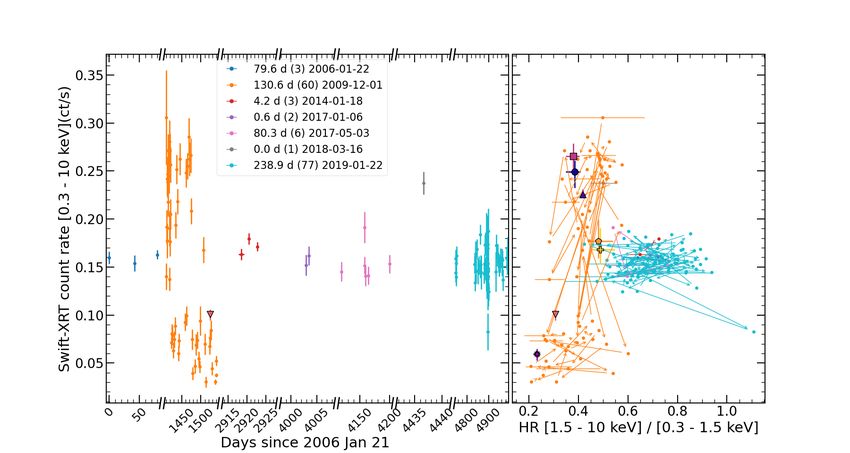
we inspected the Swift-XRT light curves and built HIDs for both The XMM–Newton observations from Figure 3 (coloured mark-
sources (Figure 1). Here we considered the data binned by ob- ers) show how the source went from the hard/intermediate state
servations to ensure that the source was well detected in each of (epoch 2003-01-06) to the soft/bright state and started transit-
the energy bands. ing from soft/bright to soft/dim from epoch 2003-05-01 onward.
The Swift-XRT data for Holmberg II X–1 reveals two dis- Another transition from bright/soft to hard/intermediate was also
tinct trends, one from the 2009/2010 data in which the source observed by XMM–Newton in 2006. Given that the source was
switched quickly and repeatedly, within a few days (see also found in the soft/dim state in 2001 and back in that state in 2003-
Grisé et al. 2010) between a bright and soft state (soft/bright 08-06 (Figure 3), the full cycle seems to have a duration of less
state: HR ∼ 0.5, count rate in the 0.3 – 10 keV band ∼ 0.28 than 2 years. It is also observed that NGC 5204 X–1 was not
cts/s) and a dim and softer state (soft/dim state: HR ∼ 0.25, detected in the soft/dim state by Swift-XRT.
count rate of ∼ 0.05 cts/s). This variability is also observed intra- Overall, the multi-instrument data presented reveals that the
observation in the long (30 ks good exposure; Gúrpide et al. evolution of both NGC 5204 X–1 and Holmberg II X–1 are akin
2021) obs id 0561580401 (this observation is indicated as a pink and can be characterized in three states: soft/bright, soft/dim
triangle pointing downwards in Figure 1). and hard/intermediate. The 2006 transitions of NGC 5204 X–1
The second trend is well sampled in the 2019 monitoring were also discussed by Sutton et al. (2013) and thus it is easy
and shows that the source remained stable with HR ∼ 0.75 and to see that the soft/bright state corresponds to the soft ultra-
a 0.3–10 keV count rate of ∼ 0.15 – 0.2 cts/s (hard/intermediate luminous (SUL) regime defined by these authors, whereas the
state). The source has been repeatedly observed in this state on hard/intermediate states correspond to the hard ultraluminous
several occasions prior to 2019, in 2006, 2014 and 2017. From (HUL) regime. The soft/dim state shows instead several char-
the 2009/2010 monitoring, the duration of whole soft state tran- acteristics similar to the supersoft ultraluminous (SSUL) regime
sitions seems to last at least ∼ 131 days, whereas the 2019 moni- (Feng et al. 2016; Urquhart & Soria 2016; Pinto et al. 2017),
toring indicates that the duration of the hard state seems to be of namely a luminosity around 1039 erg/s (Figure 3) and little emis-
at least ∼ 240 days. sion above 2 keV (see Figure 6 in Gúrpide et al. 2021). To illus-
The identification of any pattern in the Swift-XRT data is trate this further, we measured net count rates in the same three
not straightforward in the case of NGC 5204 X–1 because Swift energy bands as Urquhart & Soria (2016): 0.3.–1.1 keV (S ), 1.1–
caught the source mostly in the hard/intermediate state, albeit 2.5 keV (M) and 0.3–7.0 keV (T ). We computed (M − S )/T for
Gúrpide et al. (2021) showed that Holmberg II X–1 and NGC each of the XMM–Newton and Chandra observation available for
5204 X–1 evolved in a similar manner from the analysis of each state (Table 1). We see that the values for the soft/dim state
archival XMM–Newton and Chandra data. To illustrate this, we of NGC 5204 X–1 reach (M − S )/T ≈ – 0.8, the approximate
adapted Figure 6 from Gúrpide et al. (2021) in Figure 3 by con- threshold the authors used to classify ULX sources as super-
sidering the full Chandra monitoring of NGC 5204 X–1 pre- soft. The lowest value of Holmberg II X–1 registered by XMM–
sented by Roberts et al. (2006) (see Table 2), to highlight the Newton is –0.5, which overlaps with some supersoft sources,
short-term variability the source underwent in 2003. We fitted depending on the model considered (see their Figure 1). Note
these new Chandra observations using the same model as in also that Swift observed Holmberg II X–1 at even lower fluxes
Gúrpide et al. (2021), an absorbed dual-thermal component in than those observed by XMM–Newton (Figure 1) and that Holm-
XSPEC (Arnaud 1996) version 12.10.1f. We fixed the galactic berg II X–1 is generally softer than NGC 5204 X–1(Gúrpide
nH and the local nH to the same values found in Gúrpide et al. et al. 2021), suggesting that these differences in (M −S )/T might
(2021). The best-fit parameters are summarized in Table 3. For be mostly instrumental and that the properties of the SSUL state
our purpose, we retrieved unabsorbed fluxes using cflux in the are broader than based on hardness alone. We discuss in Sec-
0.3 – 1.5 keV and the 1.5 – 10 keV bands and show them to- tion 4 why Holmberg II X–1 and NGC 5204 X–1 appear slightly
gether with the previous observations from Gúrpide et al. (2021) harder in the SSUL state than canonical ULS sources.
in Figure 3. Additional evidence for the similarity between these states
To put the XMM–Newton and Chandra observations from and the ULS regime comes from the rapid < 2 day variability ob-
Gúrpide et al. (2021) in perspective with respect to the served in the soft/bright to soft/dim transitions in the Swift-XRT
Swift-XRT data, we estimated the count rates in the 0.3 light curve of Holmberg II X–1 (see also Grisé et al. 2010). This
– 1.5 keV, 1.5 – 10 keV and 0.3 – 10 keV bands from is reminiscent of the transitions observed in the ULS in M81 (Liu
the best-fit model parameters from Gúrpide et al. (2021) 2008), which shows sudden flux drops and rises on timescales of
by convolving each model with the latest redistribution ∼ 1 ks, similar to those seen in Holmberg II X–1 (Figure 2).
matrix (swxpc0to12s6_20130101v014.rmf) and ancillary file The ULX-ULS transitions seen in NGC 247 ULX-1 and NGC
(swxs6_20010101v001.arf) available as of 01/08/2020. In order 55 ULX are also associated with the brightest states (Feng et al.
to derive the uncertainties, we linearly interpolate the 1σ uncer- 2016; Pinto et al. 2017, 2021), which is exactly what is observed
tainties from the observed fluxes to convert them to equivalent in Holmberg II X–1 and NGC 5204 X–1. Thus, Holmberg II X–
Swift-XRT count rates. This is represented in Figure 1 using the 1 and NGC 5204 X–1 may be the first ULXs observed to switch
same colour code as in Gúrpide et al. (2021) in the case of Holm- through all these three canonical ULX spectral states. Hereafter
berg II X-1 and as Figure 3 in the case of NGC 5204 X–1. we will use the terms SUL, HUL and SSUL to refer to the spec-
Article number, page 4 of 16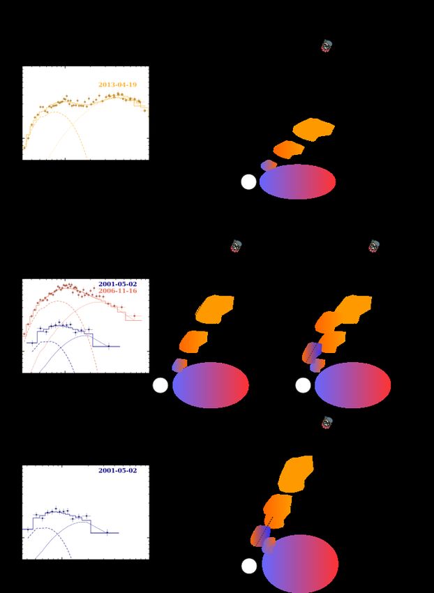
A. Gúrpide et al.: Evolutionary cycles in the ULXs Holmberg II X–1 and NGC 5204 X–1

Fig. 1. Left: Swift-XRT light curve in the 0.3 – 10 keV band for Holmberg II X–1 (top) and NGC 5204 X–1 (bottom) with its associated HID
(right). Continuous monitoring intervals with data gaps of less than 12 weeks have been coloured accordingly and the legend indicates the duration
in days, the number of observations and starting date of each continuous period. Arrows in the HID indicate chronological order and errors are
given every eight datapoints for clarity. Big coloured markers correspond to the Swift-XRT 0.3–10 keV count-rate estimates of the XMM–Newton
and Chandra observations based on best-fit models from Gúrpide et al. (2021) (see text for details). Errors are at 1 σ confidence level. Note that
the X-axis has been split on the left panels.

                                                                                                                     Article number, page 5 of 16
A&A proofs: manuscript no. aanda
Table 3. Results of the fit of the Chandra observations considered in this work that were not included in Gúrpide et al. (2021). Errors are quoted
at the 90% confidence level. The number of Cs indicates the number of observations jointly fitted.
Epoch kT soft norm kT hard norm Lasoft Lahard Latot C-stat(dof)
keV keV 10−2 (0.3–1.5 keV) (1.5–10 keV) (0.3 – 10 keV)
NGC 5204 X−1
1CC 0.26±0.03 8+6
−3 1.0+0.5
−0.2 2+4
−2 1.6±0.1 0.57+0.09
−0.08 2.2±0.1 1.24/218
2C 0.28±0.04 6+6
−3 1.2+b
−0.5 0.50+1.7
−0.5 1.4±0.1 0.4±0.1 1.8±0.2 1.03/104
3C 0.26±0.04 10+9
−4 0.9+b
−0.4 1+26
−1 1.8+0.2
−0.1 0.32+0.10
−0.08 2.1±0.2 0.79/94
Notes. The Galactic nH and the local nH were frozen to 1.75×1020 cm−2 Kalberla et al. (2005) and to 3.0×1020 cm−2 , respectively, following
Gúrpide et al. (2021). (a) I n units of 1039 erg/s. (b) W e set an upper limit of 5 keV.
Fig. 2. 0.3 – 10 keV background-subtracted EPIC-pn light curve of Fig. 3. Temporal tracks on the HLD adapted from Gúrpide et al. (2021)
Holmberg II X–1 (obs id 0561580401) binned to 500 s and corrected for NGC 5204 X–1. New Chandra observations have been included to
using the task epiclccorr. illustrate the short-term variability in 2003 (see Tables 2 and 3). Black
and coloured markers indicate Chandra and XMM–Newton observa-
tions respectively. Arrows indicate the chronological order and are only
tral states seen in Holmberg II X–1 and NGC 5204 X–1 for con- plotted for observations closer in time than 4 months.
sistency with previous works.
3.2. Periodicity analysis frequency explored to 5 days−1 , which is slightly above the typ-
ical cadence to which Swift visited each source. The minimum
3.2.1. Lomb-Scargle periodograms frequency explored is set to 1/Tsegment where Tsegment is the du-
ration of the continuous light curve segment considered in each
To investigate the presence of any periodicity in the long- case. We oversampled the periodogram by a factor five (i.e. ∆ f
term evolution of NGC 5204 X–1 and Holmberg II X–1, we = 1/nT segment where n = 5).
performed Lomb-Scargle periodograms4 (Lomb 1976; Scargle
1982), suitable to look for stable sinusoidal periodicities. In this
implementation of the Lomb-Scargle periodogram, the uncer- 3.2.2. False alarm probability: boostrap method
tainties in the measurements are used to weight the differences
between the sinusoidal model and the data, as for a classical A common challenge in the Lomb-Scargle periodogram is to es-
least-squares estimation. We also adopted the floating-mean pe- timate the significance of a peak in the power spectrum. In the
riodogram, in which the mean count-rate is fitted in the model in- presence of white noise, Scargle (1982) showed that the false
stead of being subtracted as for the classical periodogram, which alarm probability of a single peak with power P is F(P) = 1 −
has been shown to give higher accuracy, especially when the data e−P . But because we are essentially trying to detect a peak over
does not have full phase coverage (VanderPlas 2018). For this a certain frequency range, one should account for the fact that
analysis, we used the data from the Swift-XRT as it has the high- several frequencies are being explored. This is challenging be-
est cadence and longest monitoring. cause the frequencies in the Lomb-Scargle periodogram are not
In the case of unevenly sampled data, there is no well defined independent and thus one cannot compute the false alarm prob-
Nyquist frequency and thus the maximum frequency explored in ability as simply assuming that several independent frequencies
the periodogram has to be set according to some physical and/or (i.e. trials) have been looked for. Some empirical estimates of
observing constraints. In this case, we restricted the maximum the number of independent frequencies exist (e.g. Horne & Bali-
unas 1986) but the most robust method is to rely on Monte Carlo
4
https://docs.astropy.org/en/stable/timeseries/ simulations to calibrate the reference distribution, as it makes
lombscargle.html(VanderPlas 2018) few assumptions on the number of independent frequencies and
Article number, page 6 of 16A. Gúrpide et al.: Evolutionary cycles in the ULXs Holmberg II X–1 and NGC 5204 X–1
takes into account the observing cadence of the real data, so that structure from the observing window. The peaks at 444 days and
the effects of the observing window are taken into account. 103 days above the 3σ are almost exactly or very close to 2 ×
We thus estimated 2σ and 3σ false alarm probabilities in 221 days and 221/2 days respectively, suggesting that they could
the absence of a signal by using the bootstrap method outlined harmonics of the period at 221 days. The peak at 444 days is
in VanderPlas (2018). This method generates N lightcurves by also highly uncertain as it is only supported by 1.5 cycles and
drawing random samples from the original measurements to stronger noise is expected towards longer periodicities given the
generate light curves with the same time coordinates as for the sparsity of our data and the structure of the observing window.
original data. For each randomized light curve, the same Lomb- We also observe some variability on top of the sinusoidal varia-
Scargle periodogram is performed as for the real data. From tion at around 700–800 days after the beginning of the monitor-
the maxima of these fake periodograms, the reference distribu- ing.
tion is built. Another advantage of this method is that the null-
hypothesis model is not based on pure white noise, since the ref-
3.2.3. False alarm probability: REDFIT
erence distribution is built on randomized data, although there
are other limitations to consider (which we discuss in Section We note however, that in the presence of aperiodic variability,
3.2.3). We performed 3500 simulations to ensure that at least 10 the measurements could have some degree of correlation (i.e. in
peaks are found above the 3σ level and thus that the reference the presence of a flare) and by design, any correlation will be
distribution was well sampled (VanderPlas 2018). lost in the bootstrapped samples. In fact, red-noise, commonly
For Holmberg II X–1, in order to avoid aliasing effects observed in accreting sources, can often appear periodic (e.g.
caused by the large data gaps, we analysed the data separately Scargle 1981; Vaughan et al. 2016) and tests against the null-
in two segments of continuous monitoring. The first segment in- hypothesis of white noise often underestimated the false alarm
cluded the data from 2009 to 2010 and the second one comprised probability of the peaks in the periodogram (e.g. Liu 2008).
the 2019 data. The resulting periodograms are shown in Figures We therefore performed a second test to derive the signifi-
4 and 5. In the inset of the Figures we also show the structure cance of the peaks in the periodogram under the null-hypothesis
of the observing window, which is computed by performing the of red noise. To do so, we based ourselves on the publicly avail-
Lomb-Scargle periodogram on a light curve of constant flux and able R code REDFIT developed by Schulz & Mudelsee (2002)5 ,
same time coordinates as for the real data. The periodogram of in which red noise is modelled as a first-order autoregressive pro-
the 2009–2010 segment reveals two strong peaks at around 21 cess (termed AR(1) for short), a model commonly used in astro-
and 28 days both with a significance above the 3σ level. How- physics to model stochastic time-series (e.g., see Scargle 1981,
ever, the observing window has a strong power at around ∼ 25 see also An et al. (2016) for a similar approach). In AR(1) pro-
days (Figure 4), which may be introducing some aliasing. We cesses, the time series (xi ) at a given time (ti ) depend on the pre-
note also that Grisé et al. (2010) analysed the same dataset and vious sample as: xi = ρi xi−1 + i , where ρ is the autocorrelation
found no evidence for any periodicity. However, the discrepancy coefficient and is the random component with zero mean and
between these results might be simply due to the differences in a given variance σ2 . The case in which ρ = 1 simply describes
the periodogram implementation used by the authors (the pre- a random walk. For unevenly sampled data, the AR(1) can be
scription by Horne & Baliunas 1986), the sampling grid, the modelled with a variable autocorrelation coefficient that depends
way the false alarm probabilities were computed and the fact that on the sampling time difference ρ = e−(ti −ti−1 )/τ (Robinson 1977)
their implementation did not take into account the uncertainties where τ is the characteristic time of the AR(1) process, a mea-
in the measurements. sure of its memory and σ2 is set equal to 1 − e−2(ti −ti−1 )/τ to ensure
The best solution given by the 28 day peak is shown in Fig- that the AR(1) process has a variance equal to unity and is sta-
ure 4 (see the light purple solid line in the top right panel). The tionary. τ can be calculated directly from the time-series using
variability is clearly more complex than described by the simple the least-square algorithm of Mudelsee (2002). From the AR(1)
sinusoidal profile. It is also observed that the source variability model, an ensemble of Monte Carlo simulations of time series
changed after 2010-02-09 (see the blue dashed vertical line in with the same sampling as for the original light curve can be cre-
the top right panel of Figure 4). Since there is now compelling ated to test whether the presence of a peak in the periodogram is
evidence of variable periodicities in ULXs (Kong et al. 2016; consistent with an AR(1) process. However, the Lomb-Scargle
An et al. 2016; Brightman et al. 2019; Vasilopoulos et al. 2020) implementation proposed by Schulz & Stattegger (1997) does
with yet unclear origin, we repeated our analysis by considering not take into account the uncertainties in the data and the mean
separately the data before and after 2010-02-09. The results are of the measurements is not fitted as for the floating-mean peri-
presented in the top right and bottom panels of Figure 4. The odogram. Additionally, REDFIT might underestimate the signif-
peak from the first segment is consistent with the one at 28 days icance of the peaks in the periodogram as it computes the false
previously found, albeit now is found slightly below the 3σ level. alarm probabilities based on the entire distribution of the simu-
For the second segment after the blue dashed line, we found no lated periodograms, rather than on the largest peak in each syn-
evidence of any periodicity above the 2σ level. We still show the thetic periodogram.
best-solution from the highest peak found in the periodogram Because of the caveats outlined above, we replicated the
(yellow solid line in top right panel of Figure 4) to illustrate that same approach but instead simulated the ensemble of AR(1) gen-
light curves by setting the variance of the noise σ =
if the oscillation is still present, its amplitude must have signifi- 2
erated
cantly decreased. Finally, the 2019 data showed no evidence for σd 1 − e
2 −2(ti −ti−1 )/τ
, where σd is the variance of the data, so that
any periodicity which may indicate that the oscillation has de- the simulated data has variance equal to that of the real measure-
creased significantly or disappeared entirely (see Figure 5). ments. We then added an offset to the simulated data equal to the
For NGC 5204 X–1, we analysed the continuous and densely mean of the real measurements, so the simulated data has also
sampled part of the light curve from day ∼ 300 until day ∼ 900 approximately the same mean. We then computed uncertainties
after the start of the monitoring (green and purple segments in on xi assuming Poissonian statistics. In cases where xi happens
Figure 1). The Lomb–Scargle periodogram reveals a strong peak
5
at around 221 days (Figure 6), which is not coincident with any https://rdrr.io/cran/dplR/src/R/redfit.R
Article number, page 7 of 16A&A proofs: manuscript no. aanda
Fig. 4. Top left: Lomb-Scargle periodogram for the entire 2009-2010 Swift-XRT dataset of Holmberg II X-1 (black solid line). The 2σ and 3σ
levels (dashed and dotted line respectively) mark the false alarm probability computed from bootstrapped samples (see text for details). The inset
shows the structure of the observing window. Top right: Swift-XRT light curve corresponding to the 2009–2010 segment. The solid purple line
indicates the best-fit period from the periodogram of the whole light curve segment. The solid light blue line indicates the best-fit period from the
periodogram considering only the light curve segment to the left of the blue dashed line, while the yellow solid line indicates the best-fit period
from the light curve segment to the right of the blue dashed line. Bottom: Lomb-Scargle periodograms of two subsegments of the 2009–2010 data
separated by the blue dashed-line in the top right panel (left and right panels correspond to the data prior and after day ∼ 1480).
to be negative, we simply set the uncertainty equal to that of the
observed data at i. We note that there is no issue in introducing
negative rates in the Lomb-Scargle calculation, albeit ideally the
simulations should be flux limited to match more closely the real
measurements.
We then conducted the same Lomb-Scargle periodograms on
these light curves as for the real data, taking into account the
uncertainties. Following Schulz & Mudelsee (2002), we scaled
the synthetic periodograms to match the area under the power
spectrum of the real data and computed a bias-corrected version
of the periodograms. We finally derived the false alarm proba-
bility levels from each of the largest peak in the synthetic peri-
odograms. Results are shown in Figure 7 for 10000 Monte Carlo
simulations.
As expected, the false alarm probabilities under the null-
hypothesis of red noise are more stringent than those from the
bootstrap method. For Holmberg II X–1 the peak is well below
the 3σ false alarm probability. If we consider the less stringent
Fig. 5. As per Figure 4 but for the 2019 Swift-XRT dataset of Holm-
berg II X–1. false alarm probability computed from the whole distribution
of simulations (green line), the peak is only slightly below this
Article number, page 8 of 16A. Gúrpide et al.: Evolutionary cycles in the ULXs Holmberg II X–1 and NGC 5204 X–1
Fig. 6. Left: Lomb-Scargle periodogram of the 2014–2015 Swift-XRT light curve of NGC 5204 X–1 in solid black. The 2σ and 3σ mark the false
alarm probability levels computed from bootstrapped samples (see text for details). The inset plot shows the structure of the observing window.
Right: Swift-XRT light curve with the best fit period from the periodogram (orange solid line).
Fig. 7. False alarm probabilities for the Lomb-Scargle periodogram based on an adaptation of the REFIT code (see text for details) for NGC
5204 X–1 (left) for the 2014–2015 monitoring and for Holmberg II X–1 (right) for the 2009–2010 monitoring under the null-hypothesis of red
noise. The coloured 95.5% and 99.7% mark the distribution of the 10000 synthetic periodograms whereas the black dashed line 2σ and 3σ false
alarm probabilities which have been determined from the maximum of the peaks of the synthetic periodograms.
limit. It is possible that the variability exhibited by the source periodogram, and the possibility to retrieve meaningful errors
(Figure 4 right panel) is complicating the detection of the quasi- on the best period estimate, which are not well defined in the
periodicity if the latter is not strictly coherent. Thus, more mon- case of the periodogram VanderPlas (2018). We used the python
itoring might be needed to clarify whether the variability is in- implementation celerite proposed by Foreman-Mackey et al.
deed quasi-periodic. Instead, for NGC 5204 X–1 the red-noise (2017) and considered 3 different models consisting of one or
AR(1) process cannot account for the variability observed, sug- two components for our data.
gesting that the periodicity in the periodogram might be real. The first model (model a) has a single term to capture the
oscillatory behaviour by means of a damped simple harmonic
oscillator (SHO) whose power spectral density is given by:
3.2.4. Uncertainties on the period
S 0 ω40
r
In order to derive meaningful uncertainties on the periodicity 2
S (ω) = (1)
of NGC 5204 X–1, we followed Brightman et al. (2019) and π (ω2 − ω20 )2 + ω20 ω2 /Q2
used a fitting procedure based on Gaussian process modelling
proposed by Foreman-Mackey et al. (2017). Gaussian processes where S 0 is the amplitude of the oscillation, ω0 is the frequency
offer several advantages over the classical Lomb–Scargle peri- of the undamped oscillator and Q is the quality factor, which
odogram, namely, the possibility to test more refined models indicates how peaked is the periodicity in the PSD and gives a
than the implicitly assumed stable sinusoid in the Lomb–Scargle measure of the stability of the periodicity. For the second and
Article number, page 9 of 16A&A proofs: manuscript no. aanda
third models, we added a noise component on top of the SHO to and the additional Chandra and Swift-XRT data of this work. We
consider the variations not captured by the Lomb–Scargle solu- considered all the available datasets for each state, regardless of
tion (see e.g. Figure 6 around 700–800 days after the beginning their date, and fitted them assuming the same model. This selec-
of the monitoring). In one of the models this noise was modelled tion is driven by the results from Section 3.1 and the analysis
with a white noise or jitter term (model b) with amplitude σ. presented in Gúrpide et al. (2021). We also extracted Swift-XRT
For the other model (model c) we considered a red-noise com- spectra for each source state by stacking individual observations
ponent that in celerite can be modelled with the same kernel √ using the online tools (Evans et al. 2009). The count rates and
as for the damped harmonic oscillator, but fixing QN = 1 / 2 hardness used to classify the observations can be found in Table
(Foreman-Mackey et al. 2017), and leaving the other parameters 5. For NGC 5204 X–1, we found the Swift-XRT spectra of too
of the oscillator (S N , ωN ) free to vary during fit. To summarize, low data quality for a meaningful analysis. For Holmberg II X–
we thus tested three different models: a) A single SHO term, b) 1, we only found good agreement between the Swift-XRT data
the same SHO term but with a white noise term and finally c) the and the other mission datasets for the SUL regime and thus this
SHO term with the red-noise component. was the only Swift-XRT spectra that we finally used. In the other
In order to select the most suitable model for our datasets, cases we found the Swift-XRT data to be significantly dimmer
we fitted each of the three models to the light curve using the below 1 keV compared to the other datasets (residuals of & 3σ)
L-BFGS-B minimisation method from scipy and retrieved the and the floating cross-calibration constant is above 10% with re-
Bayesian information criterion (BIC) (Schwarz 1978) as given spect to the XMM–Newton data, even when taking into uncer-
in Equation 54 from Foreman-Mackey et al. (2017) i.e., lower tainties. This disagreement is consistent with the scatter seen in
BIC values indicating preferred models. We set the following the Swift-XRT observations with respect to the XMM–Newton
uniform priors on the parameters:10 < P < 700 days, 0.1 < S 0 < observations of the SSUL and HUL regimes (Figure 1).
10000 and 20 < Q < 2000. That is, all parameters are essentially We also inspected the XMM–Newton optical monitor and the
unconstrained except for the lower bound of Q, that we limited Swift-UVOT images looking for observations that could help to
as low values of Q lose the oscillatory behaviour that we want to constrain the broadband emission. However, given the limited
describe (Foreman-Mackey et al. 2017). For the red-noise com- spatial resolution of the instruments (PSF ∼ 1 arcsec) both ULXs
ponent, S N and ωN are arbitrarily started at log ωN = –0.1 and are completely blended with nearby sources in the field of view
log S N = –5 with the following uniform priors (again essentially preventing a clean determination of the direct contribution from
unconstrained): –10 < log ωN < 15 and –10 < log S 0 < 15. The the ULX. We therefore searched for Hubble Space Telescope op-
amplitude of the white noise term σ is set initially to the mean tical/UV data using the MAST portal6 and selected observations
value of the count-rate errors and is allowed to vary between –10 when the source state was known. We restricted the search to the
< log σ < 15. We performed several runs varying the initial pa- wide or medium filters as we were interested in the continuum
rameters to ensure that the minimisation routine finds the global emission. Unfortunately, we only found quasi-simultaneous HST
minimum for each model. The best-fit parameters and the BIC data for the hard/intermediate state of Holmberg II X-1 in the
calculations are presented in Table 4. F275W, F336W, F438W and F550M filters. We used a 0.255"
radius circular aperture for the source and an annulus of 0.37"
Based on the BIC values, the model with the addition of
and 0.58" inner and outer radius for the background, to consider
white noise (model b) seems the preferred model. The addition
some of the nebular emission in the background subtraction. We
of a more complex red-noise component (model c) seems not to
applied the appropriate aperture correction for each filter 7 and
be justified by the quality of data since similar solution is found
converted the telescope counts to fluxes using the calibration
as for model b (Table 4), with the addition of an extra parameter.
PHOTFLAM keywords found in the file headers8 . We obtained
Therefore, the simpler white noise component seems to be the
preferred model and we thus considered only this model for the background corrected fluxes in units of erg/cm−2 s−1 Å−1 of (6 ±
subsequent analysis. The best-fit model is shown in Figure 8. 2) × 10−17 , (3.6 ± 0.8) × 10−17 , (1.6 ± 0.4) × 10−17 and (7± 2) ×
10−18 for the F275W, F336W, F438W and F550M filters respec-
In order to estimate errors on the best fit parameters of the tively. The different datasets considered together to characterise
model with the added white noise, we initialized 32 walkers (or each state can be found in Table 1.
chains) to sample the posterior probability distribution by draw- Previous broadband spectral analysis by Tao et al. (2012) on
ing 20000 MCMC samples using the emcee library in python. NGC 5204 X–1 indicated that the emission could be consistent
Each walker is initialized by randomly drawing a sample from with an irradiated standard accretion disk and that a stellar origin
the uniform priors defined above to ensure that parameter space was unlikely. Here we chose to model our data with the physi-
is adequately sampled by the chains. In order to estimate an ad- cally motivated model sirf (Abolmasov et al. 2009, available in
equate burn-in period, we visually inspected the convergence of XSPEC), which provides a self-consistent analytical solution to
the chains and discarded the first 10000 samples of each of them. the super-critical funnel geometry based on the theoretical works
From the remaining samples, we selected one every 20 samples of Shakura & Sunyaev (1973) and Poutanen et al. (2007) to see
to derive the posterior probability density that is shown in Fig- if the broadband emission could instead be explained as arising
ure 8. The periodicity found above in the light curve of NGC from a self-irradiated supercritical disk.
5204 X–1 is found to be 197+27 −31 days (1 σ error), which is con- This model considers blackbody emission from the outer
sistent with the 221 day peak found in the Lomb–Scargle peri- wind photosphere, the walls of the supercritical funnel and the
odogram (Section 3.2.3) at the 1 σ level.
6
https://mast.stsci.edu/portal/Mashup/Clients/Mast/
Portal.html
3.3. Spectral analysis 7
https://www.stsci.edu/hst/instrumentation/acs/
data-analysis/aperture-corrections and https://www.
Here we attempt to characterize spectrally each of the states stsci.edu/hst/instrumentation/wfc3/data-analysis/
found in Section 3.1 (HUL, SUL and SSUL regimes) with a photometric-calibration/uvis-encircled-energy
physically motivated model. To do so, we made use of the XMM– 8
https://www.stsci.edu/hst/wfpc2/Wfpc2_dhb/wfpc2_
Newton, Chandra and NuSTAR data used in Gúrpide et al. (2021) ch52.html
Article number, page 10 of 16A. Gúrpide et al.: Evolutionary cycles in the ULXs Holmberg II X–1 and NGC 5204 X–1
Table 4. Best fit parameters from the minimisation routine for the three different models tested and the corresponding Bayesian information
criterion (BIC) for each of them to model the 2014–2015 light curve of NGC 5204 X–1.
Model P (days) log S 0 log Q log σ log S N log ωN BIC
NGC 5204 X–1
SHO 186.5 4.0 3.0 - - - –772
SHO + white noise 196.8 3.7 3.0 –5.1 - - –788
SHO + red-noise 196.8 3.7 3.0 - –6.9 -2.9 –783
Fig. 8. Left : Best fit solution of the celerite modelling (orange solid line) with the 1 σ shaded contours for the light curve of NGC 5204 X–
1Ṫhe model shows the SHO with additional white noise (model b), for which we only show the oscillatory component. Right: Posterior probability
distributions of the parameters of the celerite model in the right panel. The histograms along the diagonal show the marginalized posterior
distribution for each parameter with dashed lines indicating the median and the 1σ errors. The two-dimensional histograms show the marginalized
regions for each pair of parameters with the contours showing the 1 and 2 σ confidence intervals.
Table 5. Swift-XRT count rates and hardness ratios used to extract stacked spectra.
NGC 5204 X–1 Holmberg II X-1
State Count rate HR Count rate HR
cts/s cts/s
SUL 0.06–0.11 0.4–0.8 0.225–0.35 0.3–0.7
HUL 0.05–0.06 0.45–1.1 0.105–0.205 0.44–1.0
SSUL 0.4–1.1 0.035–0.05 0–0.105 0–0.8
photosphere at the bottom of the funnel, taking into account self- 1 and Holmberg II X-1, respectively; HI4PI Collaboration et al.
irradiation effects. The model has 9 variable parameters, namely, 2016) and another one free to vary. For the dataset containing
the temperature and the distance from the source of the funnel HST data, we considered interstellar extinction by adding the
bottom photosphere (T in and Rin ), the outer wind photospheric redden model in XSPEC with E(V-B) fixed to 0.074, based on the
radius (Rout ), the half-opening angle of the funnel (θ f ), the ve- measured Hα /Hβ ratio from the nebular emission of Vinokurov
locity law exponent for the wind (α) i.e., vwind ∝ rα , the adia- et al. (2013) and using the extinction curve from Cardelli et al.
batic index (γ), the mass-ejection rate (ṁejec ) and the normali- (1989) of RV = 3.1.
sation of the model. As a caveat we note that the model does The 9 parameters of the sirf model could not all be con-
not take into account Comptonization, which is likely to be an strained if left free to vary, even for the hard/intermediate state
important source of opacity in the super-Eddington regime (e.g., of Holmberg II X–1, where we had the best data quality. There-
Kawashima et al. 2012). fore, following Abolmasov et al. (2009), we fixed in all fits the
We modeled interstellar X-ray absorption with two tbabs velocity law exponent of the wind (α) to –0.5, the adiabatic in-
components, one frozen at the Galactic value along the line of dex (γ) to 4/3 and Rout to 100 Rsph , as this latter parameter is
sight (2.72 × 1020 cm−2 and 5.7 ×1020 cm−2 for NGC 5204 X– insensitive to the spectra unless its value is below 1 according
Article number, page 11 of 16A&A proofs: manuscript no. aanda
to the authors. However, we found that for the soft and super- was due to an increase of the mass-transfer rate and correspond-
soft states, due to the lack of optical coverage and the poor data ing decrease of the opening angle of the funnel, based on the
quality, we could not discriminate between different solutions, HUL-SUL softening from a rather sparse monitoring provided
with the fit often being insensitive to several parameters and re- by XMM–Newton and Chandra. The authors also suggested that
sulting in large parameter uncertainties. Another complication a line of sight grazing the wind walls in the SUL state could
arose due to the fact that the model favours solutions in which i explain the rapid transitions observed to the SSUL state as we
∼ θ f when θ f was not well constrained. This occurs due to the switch between peering down the optically thin funnel and ob-
fact that a sharp transition is created in the χ2 space when the serving the wind photosphere, as the source precessed (e.g.,
model changes from a solution where our line of sight is within Abolmasov et al. 2009). We note that a viewing angle grazing the
the the wind cone to a solution with the wind cone out of the wind walls is also supported by the lack of short-term variability
line of sight, creating an artificial minimum in the χ2 space at i in the SUL state of Holmberg II X–1 and NGC 5204 X–1 (e.g.
∼ θ f . We therefore decided to restrict the spectral analysis to the Heil et al. 2009; Sutton et al. 2013), at odds with the high-short
hard/intermediate states, which are the only states for which we term variability seen in softer soft ULXs (e.g. Middleton et al.
have broadband good quality data. Obtaining HST observations 2011) argued to be viewed through the wind. However, the lack
of both ULX in the different spectral states should help to allow of periodic variability (Figure 7) in the SUL–SSUL transitions
us to constrain the broadband emission. found here suggests that precession of the accretion flow might
The sirf model offered a good fit (χ2r = 1.00 for 960 degrees not be responsible for the spectral changes. Instead, a scenario
of freedom) to the broadband emission (see Figure 9 and Table in which the short-term variability may be ascribed to the pres-
6) of Holmberg II X–1 in the HUL state. Thus while emission ence of wind clumps crossing our line of sight (Takeuchi et al.
from the donor star or an irradiated disk could be consistent with 2013; Middleton et al. 2015a) as a result of the narrower funnel
the UV/optical emission (e.g. Tao et al. 2012), self-irradiation by is supported by the aperiodic transitions. Similar transitions from
a supercritical disk seems another plausible scenario based on SUL to SSUL are seen in the ULS NGC 247 ULX–1 (Urquhart
the broadband emission. We found an upper limit on i of 9.1◦ . & Soria 2016; Feng et al. 2016) and NGC 55 ULX (Pinto et al.
This is slightly below the lower limit of 10◦ suggested by Cseh 2017), which are also observed during the bright states (Pinto
et al. (2014), assuming that the radio jet detection is not strongly et al. 2021), suggesting a tight link between standard ULXs and
Doppler boosted, although we note that if the source precesses, ULSs. However, as opposed to NGC 247 ULX-1, Holmberg II
the viewing angle could be variable. Therefore a viewing angle X–1 and NGC 5204 X–1 are the first sources observed to switch
looking down the funnel (θ f ∼ 40 degrees) seems to be supported. through all these three canonical ULX states, possibly due to
For NGC 5204 X–1, we similarly obtained an upper limit on i the lower viewing angle compared to ULSs. Moreover, dips fre-
of ∼ 12◦ . Interestingly, the set of parameters obtained is very quently seen in ULSs (e.g. Stobbart et al. 2006; Urquhart & Soria
similar to those obtained for Holmberg II X–1, except for a fac- 2016; Alston et al. 2021) are not observed in the light curves of
tor of ∼ 7 lower ṁejec and a factor of ∼ 5 higher Rin (see Table Holmberg II X–1 and NGC 5204 X–1, supporting this interpre-
6). Therefore, the spectral differences between NGC 5204 X–1 tation. It is thus likely that the dipping activity in ULSs is asso-
and Holmberg II X–1 could be accounted by a lower ṁejec and a ciated with direct obscuration of the puffed-up accretion disk as
thicker bottom of the funnel in the case of NGC 5204 X–1 with a result of the increased mass-accretion rate (Guo et al. 2019).
an unobscured view of the bottom of the funnel in both cases. Hence the increase in mass-accretion rate confers Holmberg II
X–1 and NGC 5204 X–1 with a somewhat harder ULS aspect,
because the SSUL aspect of these standard ULXs is not due to
4. Discussion a high inclination angle, but rather due to the extreme narrowing
The multi-instrument data analysed in this work has allowed us of the funnel. This might imply that ULSs are characterized by
to firmly establish for the first time the presence of a recurrent both a high inclination angle and a high mass-accretion rate.
evolutionary cycle in ULXs. The similarities that exist in the The amplitude of the jittering decays towards the end of
temporal (Figures 1 and 3) and spectral (Figure 9 and Table 6; the 2009/2010 monitoring of Holmberg II X–1 (Figure 4).
see also Figure 6 in Gúrpide et al. 2021) properties of Holm- This might imply that the mass-transfer rate has increased and
berg II X–1 and NGC 5204 X–1 allow us to describe the evo- narrowed the funnel further, so that towards the end of the
lution of the cycle as follows: starting from the HUL state, the 2009/2010 monitoring our line of sight no longer sees the in-
sources transit to the SUL state (Figure 3). There, the sources ner regions of the accretion flow and instead mostly sees the
will transit back and forth from the SUL regime to the SSUL wind photosphere, reducing the observed variability. Such dim-
regime (Figures 1 and 3) and finally the sources will return to ming and reduced variability caused by an increase of the mass-
the HUL state from the SUL state (Figure 3). These findings of- accretion rate is in good agreement with the predictions made
fer a unique opportunity to constrain the timescale and nature of by Middleton et al. (2015a) for sources at moderate inclinations.
the transitions frequently observed in these sources (e.g., Roberts This is illustrated in Figure 10 panels b and c.
et al. 2006; Grisé et al. 2010) and could potentially be extended The spectral analysis might support a low viewing angle for
to similar transitions seen in other ULXs as well (e.g., Middleton Holmberg II X–1 and NGC 5204 X–1 at least for the HUL state
et al. 2015b; Gúrpide et al. 2021). (Section 3.3) and moderate opening angle of the funnel (θ f ∼
Spectral transitions in ULXs have been frequently discussed 40◦ ). The lack of clear jittering behaviour in the 2019 data (see
invoking geometrical effects induced by the wind/funnel struc- Figure 1) may be explained due to the larger opening angle of
ture (e.g., Sutton et al. 2013; Middleton et al. 2015a; Pinto et al. the funnel as a result of the lower mass-transfer rate. This is con-
2021) expected to form as the mass-transfer rate approaches the sistent with the reduced short-term variability seen in hard ULXs
Eddington limit and radiation pressure starts to drive a conical (e.g. Middleton et al. 2015a; Sutton et al. 2013), frequently ar-
outflow (Shakura & Sunyaev 1973; Poutanen et al. 2007). Build- gued to be viewed face-on, and is consistent with the suggestion
ing a coherent picture of the long-term spectral evolution of these that the increase of mass-transfer rate and narrowing of the open-
two ULXs was attempted in Gúrpide et al. (2021), where it was ing angle of the funnel causes the HUL–SUL spectral change
suggested that the transition from the hard to soft ULX regimes (Figure 3). This interpretation naturally accounts for the lack of
Article number, page 12 of 16You can also read