Eciency Exploration of Frequency Ratio, Entropy, and Weights of Evidence-Information Value Models in Flood Susceptibility Assessment: A Study of ...

E ciency Exploration of Frequency Ratio, Entropy,
and Weights of Evidence-Information Value Models
in Flood Susceptibility Assessment: A Study of
Raiganj Subdivision, Eastern India
Sunil Saha
 Raiganj University
Debabrata Sarkar
 Raiganj University
Prolay Mondal (  mon.prolay@gmail.com )
 Raiganj University https://orcid.org/0000-0003-3263-4377

Research Article

Keywords: Flood susceptibility mapping, Frequency ratio, Shannon’s Entropy, Weights-of-evidence, GIS,
Raiganj Subdivision

Posted Date: July 23rd, 2021

DOI: https://doi.org/10.21203/rs.3.rs-729511/v1

License:   This work is licensed under a Creative Commons Attribution 4.0 International License.
Read Full License

1   Efficiency Exploration of Frequency ratio, Entropy, and Weights of evidence-Information
 2   Value models in flood susceptibility assessment: A study of Raiganj Subdivision, Eastern
 3   India

 4   Sunil Sahaa , Debabrata Sarkarb , Prolay Mondalc*
 5   aResearch Scholar, Department of Geography, Raiganj University, Raiganj, West Bengal,
 6   733134, India. E-mail: sahasunil2507@gmail.com
 7   bResearch Scholar, Department of Geography, Raiganj University, Raiganj, West Bengal,
 8   733134, India. E-mail: debabratas077@gmail.com
 9   cAssistantProfessor, Department of Geography, Raiganj University, Raiganj, West Bengal,
10   733134, India. E-mail: mon.prolay@gmail.com
11   *Corresponding Author

12   Abstract

13   The primary objective of this research was to assess the efficiency of RS and GIS for
14   predicting the flood risk using the Frequency ratio, Entropy index, and Weight of evidence-
15   information Value models. Consequently, for spatial analyses fourteen flood conditioning
16   variables are constructed. The research region is experiencing floods consequently in the
17   past with moderate to high intensities. The assessment demonstrates that parameters such
18   as elevation, LULC, rainfall, distance from rivers, and drainage density contributed
19   significantly to the occurrence of floods. The validation of the results indicates that the
20   success rate of the presently constructed models. Around 33 per cent to 47 per cent of the
21   total area of each block in the subdivision is projected to be in danger of floods. The report's
22   findings will aid planners in designing flood prevention measures as part of regional flood
23   risk management programs and will serve as a platform for future research in the study
24   area.

25   Keywords

26   Flood susceptibility mapping, Frequency ratio, Shannon’s Entropy, Weights-of-evidence, GIS,
27   Raiganj Subdivision.

28   1. Introduction

     1|Page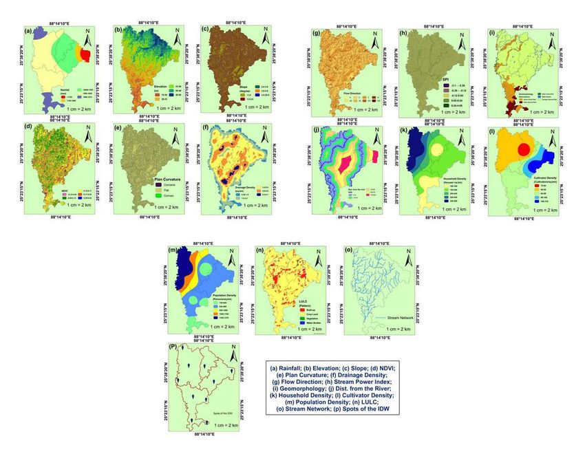

29   Flood is the most common and destructive weather phenomenon in India. Furthermore,
30   second to Bangladesh, the most flood-affected country in the world is India with around
31   one-eighth of its total land (40 million hectares) susceptible to flooding. The Central water
32   commission (2010) estimated about 7.6 million hectares of geographical area are severely
33   affected due to flooding each year. Between 13 years (1965-1978) the flood-affected area
34   has been significantly increased from 7.6 million to 17.5 million hectares. Monsoon rainfall
35   in India creates most of the flooding which happens in conjunction with the shifting nature
36   of monsoonal low-pressure centers and cyclones throughout the monsoon period between
37   June to September. Indian rivers namely Ganga, Brahmaputra, Mahanadi, Krishna, Kaveri
38   are known for devastating flooding, massive flooding occurs on these rivers as a
39   consequence of monsoon outbreaks.

40   Gupta et al. (2003), Singh and Kumar (2013) in their paper investigated that more than 30
41   million individuals are impacted by flooding in India and more than 1500 people are killed
42   each year, accounting for nearly one-fifth of the world deaths caused by this catastrophe.
43   According to a government estimate (CWC, 2010), floods killed over 92 thousand people
44   and cost $200 billion in economic damage over a 56-year period (1953-2009). Kalsi and
45   Srivastava (2006) reported that cyclone-induced floods in Orissa coastal area (Paradeep) in
46   1999 caused devastating damages to properties and about 10 thousand people are died
47   within two days (29 and 30 October). In Andhra Pradesh and Orissa, extremely destructive
48   and sudden floods wreak havoc on property and kill a considerable number of people (Dhar
49   et al., 1981a; WMO, 1994; Dhar and Nandargi, 2003). Due to the dam breaking as a
50   consequence of the unexpectedly severe flooding, flash floods might occur downstream.
51   Near 1979, the Machchhu dam collapsed in Morbi town in Saurashtra, destroying
52   unimaginable amounts of land, crops, animals, and almost 10000 human lives (Dhar et al.,
53   1981b; Dhar and Nandargi, 2003). A total of 34 million hectares of land is under threat of
54   flooding as per the national flood commission (NFC) in 1980 report and in the present day
55   this number significantly increases due to climate change and unpredictability. Though the
56   NFC study claimed that the government has secured 10 million hectares of land against
57   flooding, effective protection may only be available for 6 million hectares.

58   According to Cloke and Pappenberger (2009), it is somewhat impossible to completely avoid
59   or bypass the devastation of floods altogether, however, the severity of this catastrophe
     2|Page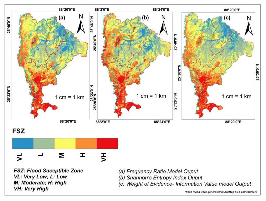

60   may be somewhat reduced by adequate risk and susceptibility assessment measures.
61   Prevention is better than quire, due to this relevance flood susceptibility evaluation and risk
62   assessment are regarded as an extremely beneficial techniques to minimize flood severity
63   (Sarkar and Mondal, 2020). In the various geospatial environments, the influencing
64   capacities of individual flood conditioning factors are different. It is thus extremely
65   important to evaluate numerous conditions that cause flood before any flood risk
66   assessments. If we consider several flood conditioning factors and performed flood
67   susceptibility mapping and risk assessment the resulted outcomes will more precise and
68   accurate rather, we use one flood-induced variable.

69   Now a day, in the field of flood susceptibility analysis, geographical information system (GIS)
70   and remotely sensed (RS) information serve as the main ingredient and achieved
71   widespread acceptance (Kafira et al., 2014; Tehrany et al., 2014; Sachdeva et al., 2017; Al-
72   Jauidi et al., 2018; Lee et al., 2018; Dano et al., 2019; Kanani-Sadat et al., 2019; Lappas and
73   Kallioras, 2019; Castache et al., 2020; Pham et al., 2020; Khoirunisa et al., 2021). The RS and
74   GIS techniques are used to gather reliable information about earth surface characteristics,
75   topographic, morphological character, LULC, meteorological information, and a wide range
76   of other associated information related to a specific environment. Concurrently, the GIS
77   platform provides a fascinating environment for flood susceptibility mapping using RS
78   datasets. The RS and GIS methodologies have effectively been used worldwide in the field of
79   flood susceptibility mapping.

80   Around the globe, the RS and GIS based different numerical, statistical and machine learning
81   methods have been used to assess flood risk and vulnerability such as, flood susceptibility
82   assessment using SVM in Kuala Terengganu (Tehrany et al., 2015), bivariate and multivariate
83   statistical approach based flood susceptibility mapping in Jeddah city (Youssef et al., 2016),
84   FR and WoE model based flood susceptibility analysis in Iran (Khosravi et al., 2016a), SEI, SI
85   and WoE model based flood susceptibility analysis in Iran (Khosravi et al., 2016b), flood
86   susceptibility analysis using FR and WoE in Iran (Golastan province) (Rahmati et al., 2016),
87   flood susceptibility mapping using hybrid AI in Haraz watershed (Chapi et al., 2017), Flood
88   risk assessment using entropy index model in Madarsoo watershed (Haghizadeh et al.,
89   2017), flood susceptibility analysis in Hengfeng using neuro-fuzzy in Hengfeng county (Hong
90   et al., 2018), flood susceptibility analysis using FR model in Markham basin, Papua New
     3|Page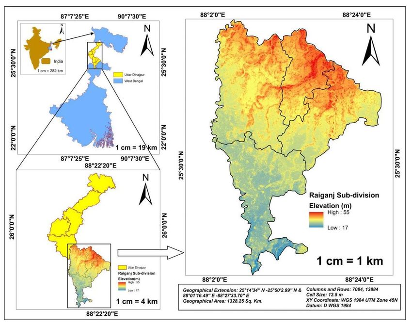

91   Guinea (Samanta et al., 2018a), flood risk assessment in Subarnarekha river basin using FR
 92   technique (Samanta et al., 2018b), flood risk evaluation using probabilistic techniques in
 93   Gucheng county (Tang et al., 2018), flood susceptibility assessment using MCDM and fuzzy
 94   in Haraz watershed (Azareh et al., 2019), fuzzy logic based flood risk assessment in Koshi
 95   river basin (Sahana and Patel, 2019), FR and LR based flood susceptibility assessment in
 96   Brisbane catchment, Australia (Tehrany et al., 2019), flood vulnerability mapping in Kulik
 97   river basin using frequency ratio model (Sarkar and Mondal, 2020), frequency ratio (FR) and
 98   SVM based flood susceptibility assessment in Sundarban BR (Sahana et al., 2020), novel
 99   ensemble and SVM based flood risk assessment (Saha et al., 2021),

100   In this present study, the bivariate techniques such as frequency ratio (FR), Shannon's
101   entropy index (SEI), and weights of evidence (WoE) were utilized along with geospatial
102   information of the study region. These bivariate methods are very effective and widely
103   accepted techniques for susceptibility analysis. The main purpose of the present study is to
104   construct and deploy a quantitative approach using bivariate techniques in conjunction with
105   RS and GIS for flood susceptibility mapping and risk assessment of the study region. For this
106   purpose, various flood conditioning parameters are taken into consideration.

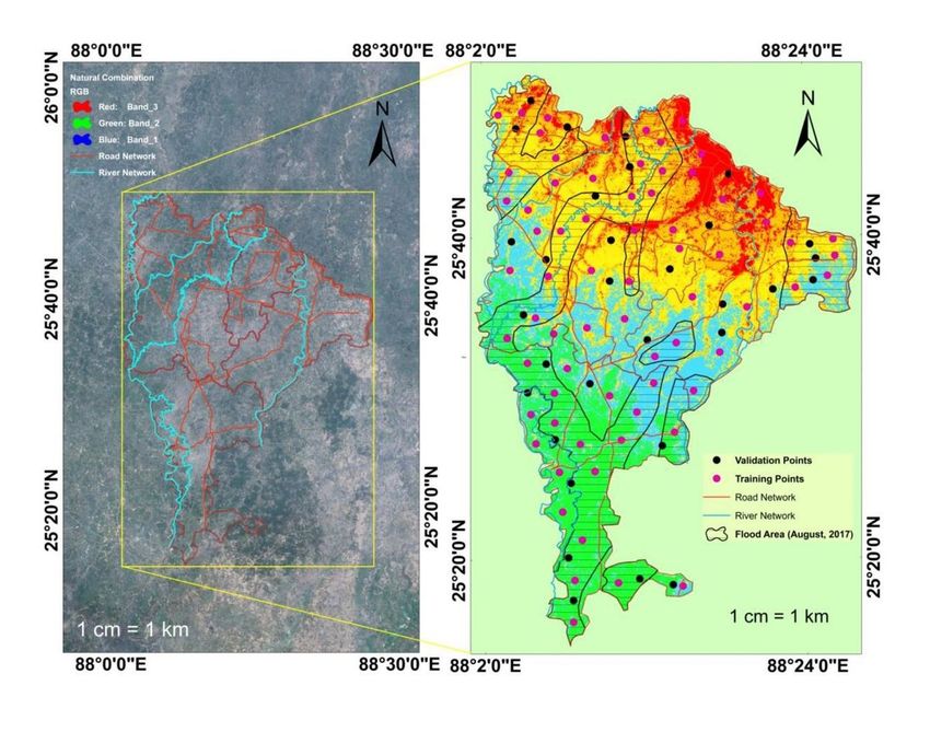
107   2. Description of the Study Area

108   Raiganj subdivision is part of Uttar Dinajpur district (Fig. 1). The Uttar Dinajpur district was
109   established on April 1, 1992, with the division of West Dinajpur into Dakshin and Uttar
110   Dinajpur, and after the formation of the Raiganj Sub-division. The research area is spread
111   out over a large geographical area with an extension of 25°14′34′′ N latitudes to 25°50′2.99′′
112   N latitudes and 88°01′16.49′′ E longitudes to 88°27′33.70′′ E longitudes. Raiganj Sub-division
113   is divided into four Community Development Blocks and four Panchayat Samitis. The study
114   area is around 1328.25 sq.km., or over 45 percent of the district's total area. Bihar in the
115   east, Malda in the south and southwest, Dakshin Dinajpur district in the east, and
116   Bangladesh in the north surround the research region. The older alluvial sediments are
117   found to be from the Pleistocene epoch. Uttar Dinajpur has been blessed with extremely
118   fertile land. The usual average high temperature is 39 °C (102 °F) in July and 26 °C (79 °F) in
119   January, owing to the sedimentary deposition that aids in the growth of rice, Jute, Mesta,
120   and Sugarcane, among other crops. The average annual temperature is around 25 ° (79

      4|Page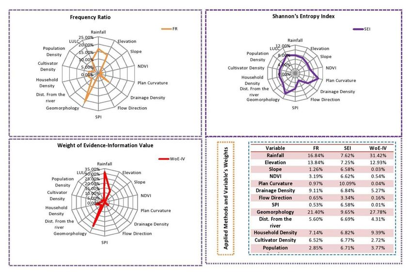

121   °). The study area is situated in the Mahananda-Nagar river basin region where the Kulik,
122   Gamari, Chhiramati (Srimati), and Tangon, Sooin (Saha et al., 2021) are major rivers flowing
123   as slope direction. In the year 2017, a major flash flood wreaked havoc in the Raiganj sub-
124   division, North Dinajpur, W/B. The destruction of the 2017 flood was caused by unplanned
125   construction, incorrect growth of the Raiganj sub-division region, and excessive rainfall in
126   adjacent states and river basins. North Dinajpur and Raiganj have previously experienced
127   floods in 1982, 1987, 1992, 1995, 1998, 2000, 2002, and 2005 and among the mentioned
128   years, the floods of 1987, 1992, 1998, and 2000 had large magnitudes and wreaked havoc
129   on the neighborhood (Saha and Mondal 2020). The flow diagram of the whole study is given
130   in Fig. 2.

131   Fig. 1 Geographical Location of the research area

132   Fig.2 Flow diagram of the research

133   3. Database and Method

134   3.1. Data Sources
135   3.1.1. Flood Inventory Map
136   The probability of a future flood event in a certain area can be predicted by looking at
137   previous flood records (Manandhar 2010). The flood inventory map (Fig. 3) is therefore
138   regarded as a significant component in predicting future floods. In this study, a flood
139   inventory map containing 70 training points was prepared using various sources of the
140   district reports. The flood inventory map was randomly partitioned into (Pradhan
141   2010; Pourtaghi & Pourghasemi 2014) two datasets such as 40 flood locations and 30 non-
142   flood locations for training and 30 validation points, respectively.
143   Fig. 3 Flood Inventory mapping of the research area

144   3.1.2. Flood predisposing Variables
145   It is believed that the precision of susceptibility simulation improves when the analysis
146   procedure integrates all event control factors. The acquisition of data and the construction
147   of databases are essential parts of any research study. There were fourteen variables
148   selected for the current simulation procedure on the expert's recommendation. The
149   simulated flood susceptibility regions of the study area were afterward determined by FR,
150   SEI, and WoE methodologies.

      5|Page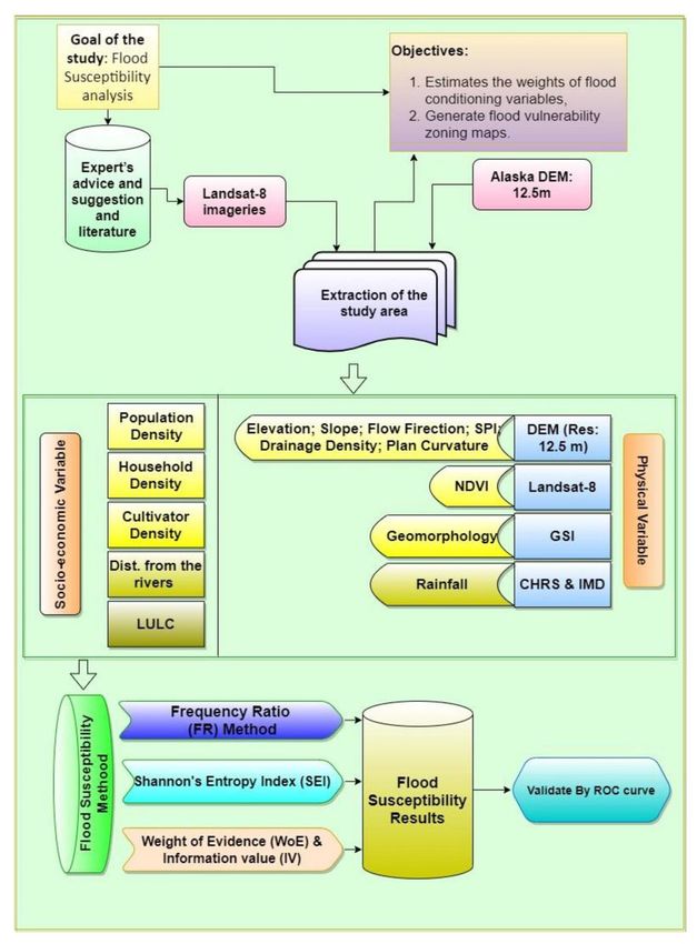

151   3.1.3. Physical Variable
152   The process of flood susceptibility mapping entails determining the flood-conditioning
153   factors (Kia et al. 2012). This study anticipates a total of 10 independent physical factors.
154   The information about rainfall was collected from the CHRS data portal and thereafter it is
155   verified with the Indian Meteorological Department’s data.
156   The Digital Elevation Models (DEMs) were downloaded from the Alaska Satellite Facility with
157   12.5 m cell size and thereafter the Elevation of the study area was estimated (Fernandez &
158   Lutz 2010).
159   Similarly, the Slope of the study area was generated using the above DEMs to access the
160   topographic inclination. The slope orientation regulates surface runoff infiltration and
161   stream flow rate of any region (Adiat et al., 2012).
162   The erosive force of surface runoff is measured using SPI. Stream Power Index (SPI) was
163   generated from the DEMs using Eq. 1.
164                          SPI  Carea  tan 
                                                             (1)
165   Where, SPI: Stream Power Index; Carea : Catchment Area (m2/m); tan  : Angle of the Slope.

166   Plan Curvature (PC), Flow Direction (FD), and Stream Density (SD) were also generated in
167   the GIS environment using Alaska DEMs. The predisposing variable that significantly
168   contributes to flooding prevalence is Stream Density (Eq. 2) (Gül 2013).

                                           slength
169                          Sdenssity 
                                                     Carea          (2)
170   Where, Sdenssity : Stream Density (km2); slength : Length of the streams in the specific

171   catchment; Carea : Catchment Area.

172   The data about geomorphology was collected from the data portal of the Geological Survey
173   of India.
174   The Normalized Difference Vegetation Index (NDVI) was estimated (Eq. 3) using the pixel
175   values of Near-Infrared Band (IR) and Red Band (RB) of Landsat-8 OLI imageries. This data
176   was collected from the USGS Earth Explorer data portal with a 30 m cell size.

177                          NDVI 
                                       NIR  RED    Band 5  Band 4 
                                       NIR  RED   Band 5  Band 4       (3)
178   Where, NDVI: Normalized Difference Vegetation Index; NIR: Near-Infrared Band.

      6|Page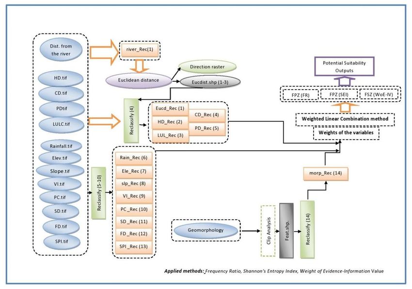

179   3.1.4. Socio-economic Variable
180   In order to evaluate the probable flood sensitivity region of the study area, some of the four
181   variables were studied from the socio-economic group. From the Census of India, the
182   statistics on population-related characteristics such as total population, total area, the total
183   number of houses, total number of farmers, were collected to estimate the Population
184   Density, Household Density, and Cultivator Density of the study area.
185   The River network of the study area was manually digitized from the Google Earth Pro
186   software to measure the distance from the river (Tehrany et al. 2015).
187   The LULC data was collected from the Bhuvan data portal and thereafter the LULC layer of
188   the study area was generated. A detailed account of variables and their sources is
189   mentioned in table 1.
190   Table 1 Data and their sources for the research work

191   3.1.5. The rationale for the Selecting of the variables
192   Rainfall is one of the prominent flood predisposing variables. Massive rainfall leads to a little
193   probability that rainwater will be absorbed by the ground (infiltration), so it will wash off
194   into the river. The quicker the water reaches the river, the greater the chance of flooding
195   (Saha et al. 2020). Excessive rainfall causes flooding when existing watercourses are unable
196   to carry the excess water (Ouma et al. 2014). The elevation influences flood vulnerability
197   (Fernandez and Lutz 2010) by regulating stream direction and producing changes in
198   vegetation and soil properties, which influence the runoff of the research area (Aniya
199   1985). Steep slopes restrict water penetration into the ground, allowing water to flow
200   quickly down to rivers as surface runoff, causing flooding. SPI was used to identify
201   and analyze areas where soil management actions could reduce surface runoff-induced
202   degradation (Jebur et al., 2014). Plan curvature is the frequency of slope changes in a
203   specific direction (Wilson and Gallant 2000) and it is also determining the flow pattern (Oh
204   and Pradhan 2011). Plan curvature measurements can be used to extract useful
205   geomorphologic data from any area. The alignment and number of cells in the catchment
206   area that contribute flow into a given cell are incorporated into the flow direction study,
207   which reflects not only the drainage network but also the route a potential flood may take
208   (Kourgialas and Karatzas 2011; Sahana et al. 2019). Geomorphology employs numerous
209   research projects, modeling, and simulation to provide a better understanding of landform

      7|Page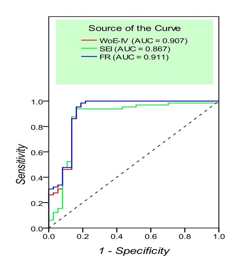

210   histories and dynamics, as well as to identify its future shifts. The variation in reflectance of
211   plant cover between visible and near-infrared wavelengths can be used to calculate the
212   density of vegetation on a plot of land (Weier and Herring, 2000).
213   The density of the population as intended is a critical measure of vulnerability because the
214   vulnerability is negligible if there is no population. Higher farmers' densities provide greater
215   assurance that crops will be destroyed during flooding. A higher density of households
216   creates a higher certainty of the destruction of houses during a flooding event. Distance
217   from the river is the most significant contributing variable due to its significant effect on
218   flood extent and intensity (Glenn et al. 2012). Improper land use and land cover pattern can
219   entertain every type of susceptibilities to occur. The most common land-use types within
220   the study area are cropland, Vegetation, bare land, built-up land, and water body. Surface
221   runoff and floods are increased in built-up areas, which are primarily made up of
222   impermeable surfaces (Tehrany et al. 2013). Due to the positive link between infiltration
223   capability and vegetation density, however, vegetated areas are less prone to flooding.
224   3.2. Methods of the study
225   3.2.1. Frequency Ratio Method (FR)
226   The predictive relationship between dependent and independent variables can be easily
227   quantified using the FR model. The FR method is a Basic Statistical Analysis method that
228   assesses the impact of each type of conditioning factor on projected flooding (Lee et al.,
229   2012; Sarkar and Mondal 2020). According to Bonham-Carter (1994), FR is the possibility of
230   the emergence of a certain event and it reveals the relationship between the flood sites and
231   their relevant variables.

232   This approach has been employed in several natural catastrophe circumstances including
233   the estimation of groundwater potentiality (Manap et al., 2014), to estimate the blast-
234   induced air-blast (Keshtegar et al. 2019), landslide susceptibility mapping (Lee and Pradhan
235   2007; Mondal and Maiti 2013), and flood susceptibility mapping (Lee et al., 2012; Rahamti
236   et al. 2015; Khosravi et al. 2016). The advantage of this model is that it is easy to apply and
237   gives totally understood outcomes (Ozdemir and Altural 2013). Among numerous bivariate
238   statistical approaches, the FR model was used in the current study to assess the flood
239   susceptibility tendency of the study area (Althuwaynee et al. 2014). This method can be
240   expressed by equation 4.

      8|Page

Pixiv
                     Pixic
241   FR                                     (4)
             Pixtv
                     Pixtc

242   Where, FR: Frequency Ration; Pixiv : Total vegetable pixel of ith alternative; Pixic : Total class

243   pixel of ith alternative; Pixtv : Total vegetable pixel of the criteria; Pixtc : Total pixel of the

244   criteria.

245   In order to assess the association between the flood site and predictor classes, the Relative
246   Frequency Index (RF) was used. It is the normalized values of the previous frequency ratio
247   (FR) values of the variables. Eq. 5 demonstrates the formulation of FRF for a given class
248   factor field.

             FRi
249   RF                         (5)
                      FR    c

250   Where, RF: Relative Frequency; FR: Frequency Ratio; FRi : FR value ith alternative;        FR   c
                                                                                                           :

251   Summation of FR values of C criteria.

252   The prediction rate was determined using equation 3 to recognize the relational
253   interrelationships among the independents. The entire procedure can be based on a
254   frequency ratio (FR) model and the individual rating of variables was expressed as the
255   prediction rate (Eq. 6) (Sabatakakis et al., 2013).

           PR 
                      MaxRF  MinRF 
256
                       Min MaxRF  MinRF 
                                                     (7)

257   Where, PR-Prediction Rate; MaxRF -Highest value from the RF values; MinRF -Least value

258   from the RF values; Min MaxRF  MinRF  - is the minimum value from all selected variables

259    MaxRF  MinRF  .

260   The flood susceptibility was calculated using a factor analysis algorithm that projected the
261   probable influence and predictor interrelationships as a function of factor analysis. The
262   following (Eq. 7) is the proposed algorithm, which combines the amount of the products of
263   fourteen separate factor variables.

      9|Page

FSZ  V1 PR  V2PR  .......VnPR
264
      Where, V1 PR  VaSlope          n
                         RF .........V PR    (7)

265   Where, FSZ: Flood Susceptibility Zone; V: Variable; PR: Prediction Rate; a: Alternatives of
266   specific variables; RF: Relative Frequencies of the alternatives of that specific variable.

267   In each area of pixels, the Flood Susceptibility Zone (FSZ) was generated independently from
268   relative frequency values of the selected fourteen conditioning variables. Following that, the
269   pixel values were classified using a natural break classification scheme (Moghaddam et al.,
270   2013) in the ArcMap-10.5 environment.

271   3.3.2. Shannon Entropy Weight Method

272   Entropy is the measure of unpredictability, volatility, imbalanced behaviors, energy
273   distribution, and instability in a system (Pourghasemi et al. 2012; Khosravi et al. 2016).
274   Stephan Boltzmann was the first to propose this theory, while Shannon was the first to
275   present it statistically in 1948. Based on the Boltzmann theorem, Shannon expanded the
276   entropy model for information theory. The entropy model has been widely used in hazard
277   identification and risk management studies to calculate the leverage ratio of natural hazards
278   and to represent the priority of some variables in influencing a particular hazard (Al-Hinai et
279   al. 2021). The core aim of this research work is to measure flood susceptibility of the study
280   area using the entropy technique. The following Eq. 8 was used to normalize the arrays of
281   performance indices to obtain the probability density.

                 FRij
282   Pdij    mj                   (8)
                FR
               i 1
                        ij

283   Where, Pdij : Probability Density or Project outcomes; FRij : Frequency Ratio value of the

284   specific cell.

285   After calculating the probability density, the entropy measure of these probability densities
286   is estimated using equation 9.

      10 | P a g e

mj

      Ev j   Pdij log 2 Pdij , j  1,..., n
287             i 1                                           (9)
      Ev j max  log 2 m j

288   Where, Ev j & Ev j max : Entropy Value;        mj   : Number of classes.

289   Furthermore, the weights of the criteria were estimated using Equations 10 and 11.

              Ev     Ev j     
290   Ic j   j max            , I  (0,1)1 j  1,....n           (10)
              Ev j max
                               

291   Cwj  I j FR              (11)

292   Where, Ic j : information coefficient; Cw j : Weight of the criteria.

293   The criteria weights of all criteria were estimated using Shannon’s entropy technique on MS
294   Excel. After calculating the entropy values, the final flood vulnerability map was generated
295   using the raster calculator tool in the ArcMap environment.

296   3.3.3. Weight of Evidence and Information Value (WoE-IV)

297   WoE is a quantitative data-driven strategy for predicting the recurrence of events based on
298   the Bayes rule (Rahmati et al., 2016). This approach, which is based on the Bayesian
299   probability model, has more facilitation when compared to other statistical methods
300   (Tehrany et al., 2014). The WoE model is built around the concept of determining positive
301   and negative weights. Based on the presence or absence of cultivations inside a certain
302   area, the approach estimates the weight of each cultivation conditioning variable. In this
303   study the following Eq. 12 was used to predict the WoE values.

      WoE  ln               
                  % Pixt
304                                        (12)
                        % Pixv

305   Where, WoE : Weight of Evidence; ln : Natural Log; % Pixt : Percentage of the total pixel of

306   the alternative; % Pixv : Percentage of the vegetable pixel of the same alternative.

307   A negative weight (W-) reflects the magnitude of negative association and implies the
308   absence of the conditioning variable and a positive weight ( W+) denotes the presence of

      11 | P a g e

309   the conditioning factor at the cultivation sites, and its magnitude reflects the positive
310   association between the presence of the conditioning component and vegetable cultivation
311   (Pradhan et al. 2010).

312   One of the most useful techniques for selecting important variables in a predictive model is
313   information value (IV). It facilitates the classification of variables according to their
314   importance. The IV is determined using the formula below (Eq. 13).

      IV   % Pixt  % Pixv   ln               
                                       % Pixt
315                                                                        (13)
                                             % Pixv

316   Where, ln : Natural Log; % Pixt : Percentage of the total pixel of the alternative; % Pixv :

317   Percentage of the vegetable pixel of the same alternative.

318   3.3.4. Weighted Linear Combination Method (WLCM)
319   Several scholars have used AHP to investigate the 'Potentiality' of its effective mathematics
320   qualities (Triantaphyllou and Mann, 1995; Srdevic et al. 2011). ‘WLC’ or ‘The 'Weighted
321   Linear Combination Model' (Fig. 8) is intended to rank the criteria in order to get a probable
322   appropriateness index. The priority values of the parameters were evaluated using AHP, and
323   then the Potential Suitability Zoning map was produced utilizing equation 14 in a GIS
324   environment.
325   FSZWLC  Variable  Rating1   .... Variable  Rating n 
                                                                     (14)
326   Where, FSZ : Flood Susceptibility Zone; WLC : Weighted Linear Combination; n : no. of the
327   variable
328   4. Discussion of the results

329   4.1. Execution Frequency ratio model

330   The FR approach was used to determine the degree of correlation between flood sites and
331   conditioning factors i.e. the frequency ratio model can be used to evaluate the correlation
332   between each flood factor and the distribution of prior floods, which is based on
333   probabilistic (statistical) methodologies (Manandhar 2010; Sarkar and Mondal 2018). Table
334   2 shows the results of the geographic connection between the flood location and the
335   conditioning factors using the FR model. In general, an FR value of 1 indicates that flood
336   sites and affective factors have an average correlation (Pradhan 2010). There is a high

      12 | P a g e

337   correlation if the FR value is greater than 1 and a lesser correlation if the FR value is less
338   than 1.

339   The relative frequencies of all variables were estimated using equation 5 which is helpful in
340   the calculation of priority values of the individual variable. A higher value of RF depicts a
341   higher susceptibility to flooding and vice-versa. The estimation of FR (RF) for the relationship
342   between flood sites and rainfall, it is found that the rainfall zone (Fig. 4a) of

368   Rainfall, Household Density, Cultivator Density, and Population Density were generated in
369   the GIS environment using the IDW tool (Fig. 4p). The correlation between flood sites and
370   the land use pattern (Fig. 4n) indicates that water bodies and cropland have a higher chance
371   to flood followed by the Built-up area.

372   The variables-wise weighting was estimated using relative frequency values where
373   Geomorphology is the most influencing variable with a priority value of 21.40 per cent
374   followed by Rainfall, Elevation, and LULC with priorities values of 16.84 per cent, 13.84 per
375   cent, and 10.10 per cent. SPI (Fig. 4h; Fig. 4o), Flow Direction, and Plan Curvature are the
376   least influencing variables to flood with 0.53 per cent, 0.65 per cent, and 0.97 per cent
377   variable priorities values.

378   Finally, the Flood Susceptibility Zoning map (Fig. 5a; Table 3) was generated using equation
379   14 in the GIS environment. From the result, it is found that 11.02 per cent of the total area is
380   very highly susceptible to flood whereas only 8.80 per cent area is least susceptible. 32.06
381   per cent of the total area is moderately susceptible to flood.

382   4.2. Execution Shannon Entropy Index

383   The relative frequency values were used to calculate the Shannon’s Entropy Index to
384   estimate the priority weights of the variables. A higher relative frequency value indicates a
385   higher probability of the flood occurring and a lower value indicates a lesser probability to
386   flood occurring. From the estimation of the relationship between the flood sites and
387   variables, it is found that the rainfall zone of

398   with a 3.34 per cent criteria weight. The rainfall and Elevation influence the estimation with
399   7.62 per cent and 7.25 per cent of criteria weights respectively.

400   Finally, the Flood Susceptibility Zoning map (Fig. 5b; Table 3) was generated using equation
401   14 in the GIS environment. From the result, it is found that 13.90 per cent of the total area is
402   very highly susceptible to flood whereas only 7.20 per cent area is least susceptible. 31.44
403   per cent of the total area is moderately susceptible to flood.

404   4.3. Execution Weight of Evidence model

405   According to Armaş (2012), WofE is one of the most extensively used statistical data
406   integration methods since it can be utilized with only a few predictive variables. According
407   to Rahmati et al. (2015), the WoE method is an appropriate technique for flood hazard
408   modeling, because its unpredictability is related to hazard events and their connections with
409   the complex landscape. From the calculation, it was found that the rainfall zone of 1750-
410   1800 mm (WoE: 0.023243), and 1800-1850 mm (WoE: 0.994778) are positively correlated
411   with flood occurrence in the study area. In the case of elevation, the zone of 40-55 m is
412   positively co-related with the flood with WoE 1.01696. The slope zone of

428   The WoE values are used to estimate the Information Values (IV) of the variables as well as
429   of all the alternatives of the variables.       Using Information Values, the final flood
430   susceptibility map was generated. The IV of rainfall is 31.42 per cent followed by
431   geomorphology with 27.78 per cent, elevation with 12.93 per cent whereas SPI represents a
432   lower IV of 0.01 per cent followed by slope with 0.03 per cent respectively.

433   Finally, the Flood Susceptibility Zoning map (Fig. 5c; Table 3) was generated using equation
434   14 in the GIS environment. From the result, it is found that 11.50 per cent of the total area is
435   very highly susceptible to flood whereas only 8.08 per cent area is least susceptible. 31.46
436   per cent of the total area is moderately susceptible to flood.

437   Fig. 4 Performing Variables of the research; (a) Rainfall; (b)Elevation; (c) Slope; (d)NDVI;
438   (e)Plan Curvature; (f) Stream Density; (g) Flow Direction; (h) SPI; (i) Geomorphology; (j) Dist.
439   from the river; (k) Household Density; (l) Cultivator Density; (m) Population Density; (n)
440   LULC; (o) Stream Network; (p) Spots of the IDW.

441   Table 2 Areal distribution of the variables with their relative weight of applied statistical
442   methods

443   4.4. Comparison of FR, SEI, and WoE-IV results

444   The final results of all the models that were applied in the evaluation nearby represent a
445   valid result. From the result changing matrix of FR and SEI, it is found that in the case of SEI
446   estimation the very high susceptibility zone is larger than 2.88 per cent from FR estimation.
447   The very low, Low, and Moderate susceptibility regions decreased in SEI estimation by -1.60
448   per cent, -3.32 per cent, and -0.62 per cent respectively. The result of WoE-IV is also valid
449   with FR estimation, where the higher flood susceptibility region is just 0.48 per cent more
450   than the FR result. The result of SEI and WOE-IV are also comparing using changing matrix
451   (Table 4; Fig. 7). The very high flood susceptibility region of the WoE-IV estimation is - 2.40
452   per cent lower than SEI estimation (Table 5).

453   Table 4 Changing comparison matrix of different alternatives of the FSZ (Flood Susceptibility
454   Zone) for applied techniques

455   Table 5 Areal changes of the result of using the methods

      16 | P a g e

456   Fig. 5 Potential Flood Susceptibility Outputs; (a) Frequency Ratio; (b) Shannon’s Entropy
457   Index; (c) WoE-IV

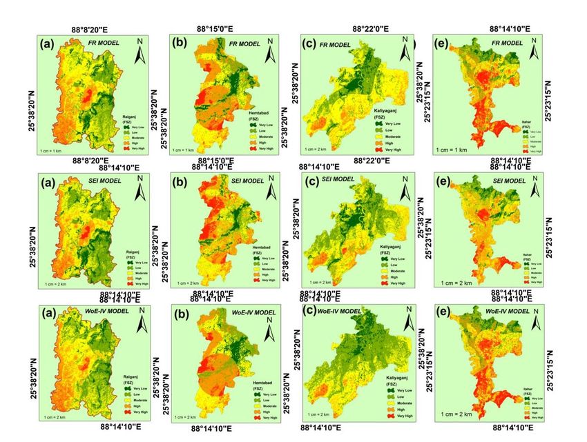
458   4.5. District-wise Flood Susceptibility Analysis

459   From the estimation of district-wise flood susceptibility regions, it is found that more than
460   33.39 per cent areas of the entire blocks are vulnerable to flood (Fig. 6). The middle,
461   western and south-western portions of the Raiganj block are highly susceptible to flood. The
462   southern and western portion of the Hemtabad block has very high susceptibility to flooding
463   during the opposite time. The Kaliyaganj block is the least flood-affected region whereas
464   only 8.16 per cent of the total area falls under the very high flood susceptibility zone. Most
465   probably, itahar is the most vulnerable block to flood where 52.34 per cent of the total area
466   falls under the very high flood susceptibility region. The southern and middle itahar is highly
467   susceptible to flood during the rainy season.

468   Fig. 6 Block-wise flood susceptibility mapping; (a)Raiganj; (b)Hemtabad; (c)Kaliyaganj; (d)
469   Itahar

470   Fig.7 Efficiency Comparison of applied methods

471   Fig. 8 Weighted Linear Combination model for potentiality estimation

472   5. Validation of the flood susceptibility maps

473   The principal objective is to find areas that may be affected by future flooding in the analysis
474   of susceptibility to floods. So it is very crucial to check the resulting flood susceptibility maps
475   in respect of any further unknown floods regardless of whether integration process is
476   employed (Chung & Fabbri 2003). The examination of the accuracy of the flood
477   susceptibility maps obtained using FR, SEI, and WoE-IV models was conducted using the
478   Receiver Operating Characteristics (ROC) analysis (Rahmati et al., 2014; Sarkar and Mondal,
479   2020). A receiver operating characteristic curve (ROC curve) is a graph that depicts a
480   classification model's output across all classification thresholds. The ROC (Receiver
481   operating features) curve, derived from the fields of signal detection, visual representation
482   of the hit, and false-alarm rate exchange. TPR vs. FPR at different prediction thresholds is
483   plotted on a ROC curve. As the rating threshold is reduced, more objects are labeled as
484   positive, resulting in a rise in both False Positives and True Positives. It is obvious that the

      17 | P a g e

485   AUC (Area Under Curve) is around 0.911 in flood susceptibility maps, which corresponds
486   with the reliability of the forecast of 91.10 per cent by methods of the FR model (Fig. 9)
487   whereas it is 86.70 per cent and 90.70 per cent for SEI and WoE-IV estimation. Therefore,
488   the FR, SEI, and WoE-IV demonstrated almost the same and fair results based on the
489   computed AUC.

490   Fig. 9 Validation of the results using ROC curve

491   6. Conclusion

492   Floods have been labeled the world's worst and most devastating catastrophe in recent
493   years, amid several geo-environmental risks and catastrophes. Flood susceptibility mapping
494   can be used to detect flood-prone locations or regions. Flood susceptibility mapping is
495   essential for flood-prone areas to prepare for proper field management. The major goal of
496   creating a flood susceptibility map was to promote community awareness of the flood
497   threat among residents, local government, and other organizations. The current research
498   aims to define flood-prone locations in the Raiganj Sub-division by developing
499   flood susceptibility maps.     The       geospatial     technology       and       BSA-based
500   statistical methodologies were used to design and assess the results of this study. This semi-
501   quantitative and BSA-based statistical technique is useful for determining appropriate
502   flood management strategies. Based on 70 training points, The FR approach was used to
503   investigate the relationship between past flood events and the likelihood of forecasted
504   future flood episodes. From the final outputs, it is found that about 11 to 14 per cent of the
505   total area belongs to the high flood susceptibility region. The results of the FR Shannon’s
506   Entropy value and WoE-IV estimations demonstrate that variables like rainfall, elevation,
507   LULC, Geomorphology, distance from the river, and drainage density play a crucial role in
508   resulting in floods in the study region. The success rate of the frequency ratio model is
509   0.911, while the success rate of Shannon's entropy is 0.867. The success rate of the WoE-
510   IV model is 0.907 indicating that the used models for analyzing flood susceptibility of the
511   Raiganj sub-division might be considered genuine. Itahar and Raiganj blocks of the district
512   are demarcated as the area having very high flood risk potentiality. The main barrier to
513   flood susceptibility mapping is the scarcity of trustworthy flood occurrence data
514   sources, information, as well as a suitable modeling approach for replicating the findings.
515   This study demonstrates that bivariate approaches such as FR, SEI, and WoE-IV, when
      18 | P a g e

516   combined with a Geographic Information System, are always effective measures (GIS) to
517   flood susceptibility mapping. A flood management strategy includes conducting a risk
518   assessment and developing a flood susceptibility map. Developing and implementing an
519   effective flood vulnerability map can help in identifying the flood hazard zones, putting
520   adequate management systems in place and early warning systems, preparation for a swift
521   response during a flood, flood shelters, and flood rescue planning are all instances of
522   resilience methods.

523   Acknowledgments

524   The authors are grateful to acknowledge all the agencies especially, the Indian
525   Meteorological Department (IMD), Geological Survey of India, Survey of India (SOI), USGS,
526   and Alaska Sattelite Facility as sources of data required for the study. We'd like to thank Dr.
527   Gopal Chandra Debnath (Retired Professor of Visva Bharati University, W/B) for his
528   assistance with the data analysis and model validation parts.

529   Compliance with ethical standards

530   The manuscript of the research was prepared as per the Journal’s ethical standards and all
531   the authors were equally contributed to the manuscript preparation. The authors hereby
532   declared that there is no conflict of interest. During the research work, no humans or
533   animals are wounded or harmed in any way.

534   Reference

535   Adiat KAN, Nawawi MNM, & Abdullah K (2012) Integration of geographic information
536   system and 2D imaging to investigate the effects of subsurface conditions on flood
537   occurrence. Mod App Sci 6(3):11-21

538   Al-Hinai H, Abdalla R (2021) Mapping Coastal Flood Susceptible Areas Using Shannon’s
539   Entropy Model: The Case of Muscat Governorate, Oman ISPRS Int J Geoinf 10(4):252

540   Al-Juaidi AE, Nassar AM, & Al-Juaidi OE (2018) Evaluation of flood susceptibility mapping
541   using logistic regression and GIS conditioning factors. Ara J Geo 11(24): 1-10

      19 | P a g e

542   Althuwaynee OF, Pradhan B, Park HJ, & Lee JH, (2014) A novel ensemble bivariate statistical
543   evidential belief function with knowledge-based analytical hierarchy process and
544   multivariate statistical logistic regression for landslide susceptibility mapping. Cat 114 :21-36

545   Aniya M, (1985) Landslide-susceptibility mapping in the Amahata river basin, Japan. Ann Ass
546   Amer Geo 75(1):102-114

547   Azareh A, Rafiei SE, Choubin B, Barkhori S, Shahdadi A, Adamowski J, & Shamshirband S,
548   (2019) Incorporating multi-criteria decision-making and fuzzy-value functions for flood
549   susceptibility assessment. Geoca Inter 1-21

550   Bonham-Carter GF, (1994) Geographic information systems for geoscientists-modeling with
551   GIS. Comp meth geosci 13:398

552   Central Water Commission (CWC), (2010) Water and related statistics Water Resource
553   Information System Directorate. New Delhi 198–247

554   Chapi K, Singh VP, Shirzadi A, Shahabi H, Bui DT, Pham BT, & Khosravi K, (2017) A novel
555   hybrid artificial intelligence approach for flood susceptibility assessment. Envir mod soft. 95:
556   229-245

557   Chung CF, Fabbri AG, (2003) Validation of spatial prediction models for landslide hazard
558   mapping. Nat Haz 30:451–472

559   Cloke HL, & Pappenberger F, (2009) Ensemble flood forecasting: A review. J hydr 375(3-4):
560   613-626

561   Costache R, Pham QB, Sharifi E, Linh NTT, Abba SI, Vojtek M, & Khoi DN (2020) Flash-flood
562   susceptibility assessment using multi-criteria decision making and machine learning
563   supported by remote sensing and gis techniques. Rem Sens 12(1):106

564   Dano UL, Balogun AL, Matori AN, Wan YK, Abubakar IR, Said Mohamed MA, & Pradhan B
565   (2019) Flood susceptibility mapping using GIS-based analytic network process: A case study
566   of Perlis, Malaysia. Wat 11(3): 615

567   Dhar ON, Mandal BN, and Ghose GC (1981a) Vamsadhara flash flood of September 1980 - a
568   brief appraisal. Va Man 11: 7-11

      20 | P a g e

569   Dhar ON, Nandargi S (2003) Hydrometeorological aspects of floods in India. Nat Haz 28(1):1-
570   33

571   Dhar ON, Rakhecha PR, Mandal BN, Sangam RB (1981b) The rainstorm which caused the
572   Morvi dam disaster in August 1979/L'orage qui a provoqué la catastrophe du barrage Morvi
573   août 1979 Hydr Sci J 26(1):71-81

574   Fernández DS, Lutz MA (2010) Urban flood hazard zoning in Tucumán Province, Argentina,
575   using GIS and multicriteria decision analysis. Eng Geo 111:90–98

576   Glenn E, Morino K, Nagler P, Murray R, Pearlstein S, Hultine K (2012) Roles of saltcedar
577   (Tamarix spp) and capillary rise in salinizing a non-flooding terrace on a flow-regulated
578   desert river. J Ari Envi 79:56–65

579   Gül GO, (2013) Estimating flood exposure potentials in Turkish catchments through index-
580   based flood mapping Nat Haz. 69:403–423

581   Gupta S, Javed A, Dutt D (2003) Economics of flood protection in India. Nat Haz 28:199–210

582   Haghizadeh A, Siahkamari S, Haghiabi AH, & Rahmati O (2017) Forecasting flood-prone areas
583   using Shannon’s entropy model. J Ear Sys Sci 126(3): 39

584   Hong H, Panahi M, Shirzadi A, Ma T, Liu J, Zhu AX, & Kazakis N (2018) Flood susceptibility
585   assessment in Hengfeng area coupling adaptive neuro-fuzzy inference system with genetic
586   algorithm and differential evolution. Sci tot Envi 621:1124-1141

587   Jebur MN, Pradhan B, Tehrany MS, (2014) Using ALOS PALSAR derived high-resolution
588   DInSAR to detect slow-moving landslides in tropical forest, Cameron Highlands, Malaysia. J
589   Geo Nat Haz Ri 1–19. https:// doi:101080/194757052013860407

590   Kafira V, Albanakis K, & Oikonomidis D (2014) Flood Susceptibility Assessment using GIS An
591   example from Kassandra Peninsula, Halkidiki, Greece. Proc 10th Inte Congress Hel Geo Soci
592   Thessaloniki, Greece 287-308

593   Kalsi SR, & Srivastava KB (2006) Characteristic features of Orissa super cyclone of 29th
594   October, 1999 as observed through CDR Paradip. Maus 57(1):21

      21 | P a g e

595   Kanani-Sadat Y, Arabsheibani R, Karimipour F, & Nasseri M (2019) A new approach to flood
596   susceptibility assessment in data-scarce and ungauged regions based on GIS-based hybrid
597   multi criteria decision-making method. J Hydr 572:17-31

598   Keshtegar B, Hasanipanah M, Bakhshayeshi I, Sarafraz ME, (2019) A novel nonlinear
599   modeling for the prediction of blast-induced airblast using a modified conjugate FR
600   method. Mea 131:35-41

601   Khoirunisa N, Ku CY, & Liu CY (2021) A GIS-Based Artificial Neural Network Model for Flood
602   Susceptibility Assessment. Inter J Envir Res Pub Hea 18(3):1072

603   Khosravi K, Nohani E, Maroufinia E, & Pourghasemi HR (2016a) A GIS-based flood
604   susceptibility assessment and its mapping in Iran: a comparison between frequency ratio
605   and weights-of-evidence bivariate statistical models with multi-criteria decision-making
606   technique. Nat Haz 83(2):947-987

607   Khosravi K, Nohani E, Maroufinia E, Pourghasemi HR (2016b) A GIS-based flood susceptibility
608   assessment and its mapping in Iran: a comparison between frequency ratio and weights-of-
609   evidence bivariate statistical models with multi-criteria decision-making technique. Nat
610   Haz 83(2):947-987

611   Khosravi K, Pourghasemi HR, Chapi K, & Bahri M (2016c) Flash flood susceptibility analysis
612   and its mapping using different bivariate models in Iran: a comparison between Shannon’s
613   entropy, statistical index, and weighting factor models. Envi moni asse 188(12):1-21

614   Kia MB, Pirasteh S, Pradhan B, Mahmud AR, Sulaiman WNA, & Moradi A (2012) An artificial
615   neural network model for flood simulation using GIS: Johor River Basin, Malaysia. Envi Ear
616   Sci 67(1):251-264

617   Kourgialas NN, Karatzas GP (2011) Flood management and a GIS modelling method to assess
618   flood-hazard areas: a case study. Hydr Sci J 56:212–225

619   Lappas I, & Kallioras A (2019) Flood susceptibility assessment through GIS-based multi-
620   criteria approach and analytical hierarchy process (AHP) in a river basin in Central
621   Greece. para (Malczewski, 1999):6(03)

      22 | P a g e

622   Lee MJ, Kang JE, & Jeon S (2012) Application of frequency ratio model and validation for
623   predictive flooded area susceptibility mapping using GIS. Int geosci rem sens sym 895-898

624   Lee S, and Pradhan B (2007) Landslide hazard mapping at Selangor, Malaysia using
625   frequency ratio and logistic regression models Landslides. 4(1). 3341doi:101007/s10346-
626   006-0047-y

627   Lee S, Lee S, Lee MJ, & Jung HS (2018) Spatial assessment of urban flood susceptibility using
628   data mining and geographic information System (GIS) tools. Sust 10(3):648

629   Manandhar B (2010) Flood Plain Analysis and Risk Assessment of Lothar Khola, MSc Thesis,
630   Tribhuvan University, Phokara, Nepal, 64

631   Manap AM, Nampak H, Pradhan B, Lee S, Sulaiman WNA, & Ramli MF (2014) Application of
632   probabilistic-based frequency ratio model in groundwater potential mapping using remote
633   sensing data and GIS. Ara J Geosci 7(2):711-724

634   Moghaddam DD, Rezaei M, Pourghasemi HR, Pourtaghie ZS, Pradhan B (2015) Groundwater
635   spring potential mapping using bivariate statistical model and GIS in the Taleghan
636   watershed, Iran. Ara J Geosci 8(2):913-929

637   Mondal S, Maiti R, (2013) Integrating the analytical hierarchy process (AHP) and the
638   frequency ratio (FR) model in landslide susceptibility mapping of Shiv-khola watershed,
639   Darjeeling Himalaya. Inter J Dis Ris Sci 4(4):200-212

640   Oh HJ, Pradhan B, (2011) Application of a neuro-fuzzy model to landslide susceptibility
641   mapping for shallow landslides in a tropical hilly area. Comp Geosci 37:1264–1276

642   Ouma YO, & Tateishi R (2014) Urban flood vulnerability and risk mapping using integrated
643   multi-parametric    AHP     and    GIS:    methodological   overview    and    case    study
644   assessment. Wat 6(6):1515-1545

645   Ozdemir A, Altural T (2013) A comparative study of frequency ratio, weights of evidence and
646   logistic regression methods for landslide susceptibility mapping: Sultan Mountains, SW
647   Turkey. J Asian Earth Sci64:180-197

648   Pham BT, Avand M, Janizadeh S, Phong TV, Al-Ansari N, Ho, LS, PrakashI (2020) GIS based
649   hybrid computational approaches for flash flood susceptibility assessment. Water 12(3):683

      23 | P a g e

650   Pourghasemi HR, Mohammadi M, Pradhan B (2012) Landslide susceptibility mapping using
651   index of entropy and conditional probability models at Safarood Basin, Iran. Catena 97:71-
652   84

653   Pourtaghi, ZS, Pourghasemi, HR, (2014) GIS-based groundwater spring potential assessment
654   and mapping in the Birjand Township, southern Khorasan Province, Iran.Hydrogeol Jdoi:
655   101007/s10040-013-1089-6

656   Pradhan B (2010) Flood susceptible mapping and risk area estimation using logistic
657   regression, GIS and remote sensing.J Spat Hydrol 9(2):1–18

658   Rahmati O, Nazari SA, Mahdavi M, Pourghasemi HR, Zeinivand H (2014) Groundwater
659   potential mapping at Kurdistan region of Iran using analytic hierarchy process and
660   GIS.Arab J Geoscidoi: 101007/s12517-014-1668-4

661   Rahmati O, Samani AN, Mahdavi M, PourghasemiHR, Zeinivand H (2015) Groundwater
662   potential mapping at Kurdistan region of Iran using analytic hierarchy process and
663   GIS. Arab J Geosci8(9):7059-7071

664   RahmatiO, Pourghasemi HR, Zeinivand H (2016) Flood susceptibility mapping using
665   frequency ratio and weights-of-evidence models in the Golastan Province, Iran. Geocarto
666   Int31(1):42-70

667   Sabatakakis N, Koukis G, Vassiliades E, Lainas S (2013) Landslide susceptibility zonation in
668   Greece. Nat Hazards65(1):523-543

669   Sachdeva S, Bhatia T, Verma AK (2017) Flood susceptibility mapping using GIS-based support
670   vector machine and particle swarm optimization: A case study in Uttarakhand (India)
671   In 2017 8th International conference on computing, communication and networking
672   technologies (ICCCNT) (pp 1-7) IEEE

673   Saha A, Pal SC, Arabameri A, Blaschke T, Panahi S, ChowdhuriI,Arora A (2021) Flood
674   susceptibility assessment using novel ensemble of hyperpipes and support vector regression
675   algorithms. Water, 13(2):241

      24 | P a g e

676   Saha S, Mondal P (2020) A Catastrophic Flooding Event in North Bengal, 2017 and its Impact
677   Assessment: A Case Study of Raiganj CD Block Uttar Dinajpur, West Bengal. AppliGeospat
678   Tech Geomorpho Environ IGI Conf ISBN 978-81-925799-3-1

679   Saha S, Sarkar D, MondalP, Goswami S (2021) GIS and multi-criteria decision-making
680   assessment of sites suitability for agriculture in an anabranching site of sooin river,
681   India. Model Earth Syst Environ7(1):571-588

682   Sahana M, Patel PP (2019) A comparison of frequency ratio and fuzzy logic models for flood
683   susceptibility   assessment     of    the      lower   Kosi   River    Basin     in   India.
684   Environ Earth Sci78(10):1-27

685   Sahana M, Rehman S, Sajjad H, Hong H, (2020) Exploring effectiveness of frequency ratio
686   and support vector machine models in storm surge flood susceptibility assessment: A study
687   of Sundarban Biosphere Reserve, India. Catena 189:104450

688   Samanta S, Pal DK, Palsamanta B (2018a) Flood susceptibility analysis through remote
689   sensing, GIS and frequency ratio model. Appl Water Sci8(2):1-14

690   SamantaRK, Bhunia GS, Shit PK,Pourghasemi HR (2018b) Flood susceptibility mapping using
691   geospatial frequency ratio technique: a case study of Subarnarekha River Basin,
692   India. Model Earth Syst Environ 4(1):395-408

693   Sarkar D, Mondal P (2020) Flood vulnerability mapping using frequency ratio (FR) model: a
694   case study on Kulik river basin, Indo-Bangladesh Barind region. Appl Water Sci 10(1):1-13

695   Singh O, Kumar M(2013) Flood events, fatalities and damages in India from 1978 to
696   2006. Nat hazards, 69(3):1815-1834

697   Srdevic Z, Blagojevic B, Srdevic B (2011) AHP based group decision making in ranking loan
698   applicants for purchasing irrigation equipment: a case study Bulgarian. J Agric Sci17(4):531-
699   543

700   Tang Z, Yi S, Wang C, Xiao Y (2018) Incorporating probabilistic approach into local multi-
701   criteria decision analysis for flood susceptibility assessment. Stoch Environ Res Risk
702   Assess 32(3):701-714

      25 | P a g e

703   Tehrany M, Kumar L, NeamahJeburM, Shabani F (2019) Evaluating the application of the
704   statistical index method in flood susceptibility mapping and its comparison with frequency
705   ratio and logistic regression methods. Geomat Nat Haz Risk 10(1):79-101

706   Tehrany MS, Pradhan B, Mansor S, Ahmad N (2015) Flood susceptibility assessment using
707   GIS-based support vector machine model with different kernel types. Catena 125:91–101

708   TehranyMS, Pradhan B,Jebur MN (2014) Flood susceptibility mapping using a novel
709   ensemble weights-of-evidence and support vector machine models in GIS. J hydrol 512:332-
710   343

711   Triantaphyllou E, Mann SH (1995) Using the analytic hierarchy process for decision making
712   in engineering applications: some challenges. Int J Ind Eng: Theory Appl Pract2(1):35-44

713   Weier     J,Herring   D,   (2000)    Measuring     Vegetation    (NDVIEVI)    NASA     Earth
714   Observatory Washington, DC, USA

715   WHO (2003) World Health Organization Disaster data-key trends and statistics in world
716   disasters report WHO, Geneva, Switzerland

717   Wilson JP, Gallant JC (2000) Terrain Analysis: Principles and Applications New York. Wiley, p
718   479

719   Youssef AM, Pradhan B, Sefry SA (2016) Flash flood susceptibility assessment in Jeddah city
720   (Kingdom of Saudi Arabia) using bivariate and multivariate statistical models. Environ Earth
721   Sci 75(1):12

      26 | P a g e

Figures

Figure 1

Geographical Location of the research area

Figure 2

Flow diagram of the research

Figure 3

Flood Inventory mapping of the research area

Figure 4

Performing Variables of the research; (a) Rainfall; (b)Elevation; (c) Slope; (d)NDVI; (e)Plan Curvature; (f)
Stream Density; (g) Flow Direction; (h) SPI; (i) Geomorphology; (j) Dist. from the river; (k) Household
Density; (l) Cultivator Density; (m) Population Density; (n) LULC; (o) Stream Network; (p) Spots of the IDW.

Figure 5

Potential Flood Susceptibility Outputs; (a) Frequency Ratio; (b) Shannon’s Entropy Index; (c) WoE-IV

Figure 6

Block-wise ood susceptibility mapping; (a)Raiganj; (b)Hemtabad; (c)Kaliyaganj; (d) Itahar

Figure 7

E ciency Comparison of applied methods

Figure 8

Weighted Linear Combination model for potentiality estimation

Figure 9

Validation of the results using ROC curve