Exact polarization energy for clusters of contacting dielectrics
←
→
Page content transcription
If your browser does not render page correctly, please read the page content below
Exact polarization energy for clusters of contacting dielectrics
                                                                                               Huada Lian1 and Jian Qin2,*
                                                                    1
                                                                        Department of Materials Science & Engineering, Stanford University
                                                                           2
                                                                             Department of Chemical Engineering, Stanford University
                                                                                   *
                                                                                     Corresponding author: jianq@stanford.edu
arXiv:2104.04175v1 [cond-mat.soft] 9 Apr 2021

                                                                                                         April 12, 2021

                                                                                                             Abstract
                                                        The induced surface charges appear to diverge when dielectric particles form close contacts. Resolving this singularity
                                                    numerically is prohibitively expensive because high spatial resolution is needed. We show that the strength of this
                                                    singularity is logarithmic in both inter-particle separation and dielectric permittivity. A regularization scheme is proposed
                                                    to isolate this singularity, and to calculate the exact cohesive energy for clusters of contacting dielectric particles. The
                                                    results indicate that polarization energy stabilizes clusters of open configurations when permittivity is high, in agreement
                                                    with the behavior of conducting particles, but stabilizes the compact configurations when permittivity is low.
                                                For particle aggregates or clusters stabilized by electrostatic       in the electrostatic potentials of particles. This is analogous
                                                interactions, 1–3 the cohesive energy depends on the dielec-          to the divergent lubrication force between approaching solid
                                                tric permittivities of both the particles and the medium.             particles in the Stokesian regime. 15 Resolving these appar-
                                                Permittivity quantifies the density of dipoles induced by ex-         ently diverging charge densities requires a high spatial reso-
                                                ternally applied electric fields, which is proportional to po-        lution that becomes computationally prohibitive for nearly
                                                larization in the linear regime. When the permittivity con-           touching particles. 8 For conductors like metalic particles,
                                                trast between the particles and the medium is high, as is             the functional form of the divergent charge density has been
                                                often the case, the polarizations from the two sides of the           identified and used to isolate the singularity obscuring nu-
                                                interface do not fully compensate each other, resulting in            merical calculations, and to obtain the exact energy and
                                                the accumulation of induced surface charges.                          force for contacting particles. 5 For dielectric particles, the
                                                                                                                      question remains unsolved.
                                                    Resolving the surface charges is needed to evaluating the
                                                electrostatic interactions among particles in close proxim-
                                                ity, and is challenging because polarization is intrinsically a
                                                many-body effect, depending on the positions of all parti-
                                                cles. For instance, careful measurements in colloidal suspen-
                                                sions have shown that the inter-particle force is non-additive,
                                                which is at least partially due to the polarization effect. 4
                                                In another set of experiments on metallic nanoparticles, it
                                                has been found that the aggregation of multiple particles
                                                surrounding a charged particle can be stabilized by the po-
                                                larization effect alone. 3,5 More dramatic demonstration of
                                                such polarization effects is found in the so-called like-charge
                                                attraction caused by the strong polarization effect, for par-
                                                ticles of large size or permittivity ratios. 6,7
                                                    Computational methods, such as the boundary element
                                                method, 8 the spectral methods 9,10 and the image method, 11
                                                have been developed to account for this polarization effect.          Figure 1: Surface charges between two particles separated
                                                In practice, these methods all need to evaluate the induced           by a distance h. The separation of two surfaces at a radial
                                                surface charge densities in one form or another, and have             distance r from the contact points can be approximated by
                                                been successfully applied to study a wide range of prob-              h + r2 /a, where a ≡ 2/(a−1       −1
                                                                                                                                                 1 + a2 ). The permittivity of the
                                                lems involving the aggregation of polarizable particles. 12–14        medium is ǫout . Surface of conducting particles are equipo-
                                                However, when particles are in close proximity, the surface           tential with potential set to V and 0. Surfaces of dielectric
                                                charge densities apparently diverge because the electric field        particles, with permittivities ǫ1 and ǫ2 , have surface poten-
                                                in the narrow gap region is strong even for a small difference        tial distributions φ1 (r) and φ2 (r), respectively.

                                                                                                                  1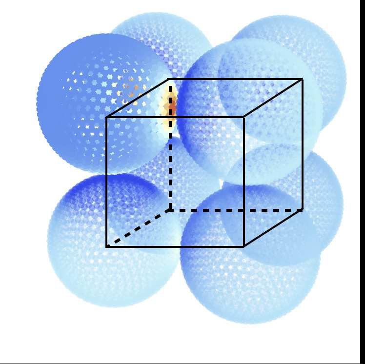
One way to reveal these singular surface charges is to               not equipotential. The potential difference ∆V (r) needed
consider two conducting particles separated by a small gap,              to evaluate the charge density in eq. (1) can not be fully
as sketched in Fig. 1. The points on the two surfaces sep-               specified by the potential difference between the contact
arated by the minimum distance, or gap distance h, are                   points ∆V (0). The variation of ∆V (r) with r in the gap
referred to as contact points. The surface charge density                region is expected to be quadratic, but the curvature is un-
is proportional to the strength of the normal component of               known a priori. In an early, and analogous work on thermal
electric field on surfaces, according to Gauss’s law. When h             conduction of composite materials, Batchelor et al. 16 no-
is small, the electric field lines in the gap region are nearly          ticed that the potential distribution, which determines the
parallel to the line connecting the two contact points. The              surface charges, is itself dominated by the contribution from
strength of the electrical field is, in turn, proportional to            the surface charges nearby, so that a self-consistent treat-
the difference in the surface electrical potentials. This re-            ment is needed.
lation between the surface potential and the electrical field                To illustrate this point, we consider the dielectric case
is analogous to that between the longitudinal velocities of              in Fig. 1. Let the surface potentials of the two particles be
converging particles and the transverse velocity of squzzed              φ1 (r) and φ2 (r), and the surface charges be σ1 (r) and σ2 (r).
fluid velocity in the lubrication theory. 15                             The surface potential φi (r), with i = 1, 2, can be calculated
    To calculate the surface charge density, both the surface            by integrating the coulombic potential of the respective sur-
potentials and the vertical separations are needed. Since                face charges. Near the contact point, we have
conductors are equipotential, the surface potentials can be                                   ˆ ∞ ˆ 2π
set to V and 0 respectively. The vertical separation de-                                  1                        r′ σi (r′ )
                                                                          φi (r) = Ṽi +          dr′   dθ′ √                        . (2)
pends on the radial distance r, and can be expressed within                              2πǫi 0       0       r2 + r′2 − 2rr′ cos θ′
the Derjaguin approximation as h + r2 /a, where a is the
harmonic average of radii of curvature a1 and a2 at the        Here, Ṽi are the contributions to the surface potential from
two contact points, i.e., a−1 = (a−1           −1
                                       1 + a2 )/2. Here, the
                                                               the surface charge outside the contact region. The integral
spherical apexes are assumed for simplicity, but more gen-     are those from the surface charges in the contact region. The
                                                                               1                   1
eral curvatures can be treated similarly. Consequently, the    prefactor is 2π      (instead of 4π   ) because of the well-known
field strength at radius r is E(r) = V /(h + r2 /a), and the   jump condition for surface potentials. 17 The distance at de-
surface charge density σ(r) = 4π  1                            nominator is approximated using that for the flat surface,
                                    ǫout V /(h + r2 /a) on the top
surface, where ǫout is the medium permittivity. Integrating    which leads to negligible error because only the contact re-
σ(r) for r from 0 to R0 , where R0 is a cutoff of order a,     gion is of concern. The upper bound is set to infinity for con-
results in the singular part of the surface charge             venience; as we shall see below, the singular surface charge
                                                               density dies off rapidly outside the contact region.
           V ǫout R0        2πr        V ǫout a  a
                  ˆ
                                                               (1) The surface charge density σi (r) in eq. (2) are related to
     Qs =              dr           ≃           ln       .
             4π    0      h + r2 /a        4         h         the potential difference, ∆V (r) ≡ φ1 (r) − φ2 (r). By analogy
                                                               to the conductor case, the electric field is approximately ver-
The unity in the logarithmic term is dropped because R0 ≃ tical and its magnitude is ∆V (r)/(h + r2 /a). Then applying
a ≫ h. Further, the difference between R0 and a is neglected Gauss’s law, we get the charge density on the top surface
because it only leads to a constant shift. Equation (1) shows
how surface charges of the upper surface become singular as                                             −1
                                                                                                             ∆V (r)
the gap distance decreases. That of the lower surface is also                  σ  1 (r) =  ǫ out 1 −  ǫ r,1            ,       (3)
                                                                                                             h + r2 /a
singular, but of opposite sign. In the limit h → 0, the energy
does not blow up because the potential difference V vanishes where ǫr,1 ≡ ǫ1 /ǫout . The charge density σ2 is given sim-
once particles form contact.                                   ilarly, but with a negative sign. Substituting the charge
    The ratio of the singular charge Qs and the potential densities to eq. (2) and taking the difference gives an inte-
difference V gives the singular part of the capacitance cs = gral equation for ∆V (r). The dependence on the unknown,
ǫout a ln(a/h)/4, which has been found previous for spherical Ṽ1 − Ṽ2 , can be factored out by introducing an auxiliary,
dimers. 6,7 The above analysis shows that this singular ca- f (r) ≡ 1 − ∆V (r)/(Ṽ1 − Ṽ2 ), which satisfies
pacitance is local. Thus, the same singularity applies to non-
spherical particles, and for aggregates of multiple particles.                 ǫ−1        −1 ˆ ∞
                                                                                 r,1 + ǫr,2             1 − f (r′ ) 4r′
                                                                      f (r) =                     dr′                    K(x). (4)
This fact has been employed to find the exact energy for clus-                       2π        0       h + r′2 /a r + r′
                                           5
ters of contacting, conducting particles. In this work, the
full capacitance array is first numerically calculated for an Here the integral over the azimuthal angle has been replaced
ensemble of conducting particles at finite but small separa- with the complete          elliptic function of the first kind K(x),
                                                                              4rr ′
tions. The singular contribution is then subtracted, leaving where x ≡ (r+r′ )2 . When ǫ1 = ǫ2 , eq. (4) reduces to Batch-
a regular part that can be extrapolated to h = 0. Finally, elor’s original result, eq. (4.5) in ref. 16. Since f (r) is pro-
when the singular and regular parts are pieced together, the portional to the contribution from the surface charges in
variation of energy with separation is obtained.               the contact region, we see that it is dominated by particles
    For the dielectric case, a straightforward generaliza- of lower permittivity. When both permittivities approach
tion of the above treatment fails, because the particles are infinity, we have f (r) = 0 and ∆V (r) = Ṽ1 − Ṽ2 , which

                                                                     2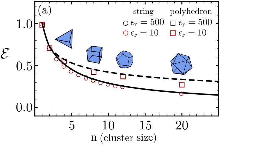
is identical to the expression for the conductors discussed
above. More general cases are discussed below.
    The solution to eq. (4) is uniquely determined by the
normalized distance h/a and the average permittivity, ǫr ≡
                                          16
2/(ǫ−1      −1
     r,1 + ǫr,2 ). As shown by Batchelor,    eq. (4) can be non-
dimensionalized to
                      1 ∞ ′ 1 − f (ρ′ ) 4ρ′
                        ˆ
             f (ρ) =       dρ                   K(x)         (5)
                      π 0       λ + ρ′2 ρ + ρ′
in which ρ ≡ rǫr /a and λ ≡ hǫ2r /a. The numerically solved
f (ρ) for a few representative λ values are shown in Fig. 2a.
For large gap distance, with λ ≫ 1, f (ρ) is nearly uniform,
as expected. For smaller λ values, f (ρ) decreases from f (0)
with r monotonically. The difference in electric potential at
the contact points is proportional to 1 − f (0). The value
of f (0) increases as h decreases, and reaches unity at h = 0,
ensuring that the surface potential is continuous at the con-
tact point. The variation of f (ρ) obtained from the above
local analysis is confirmed by directly solving the full poten-
tial distribution for dielectric dimers (inset, Fig. 2a).
     Similar to eq. (1) for the conductor case, the singular
part of surface charges on particle 1 is given, with R0 being
the regularizing cutoff of order a, by
           (Ṽ1 − Ṽ2 )ǫout            R0 2πr [1 − f (r)]
                                        ˆ
                                   −1
    Qs,1 =                   1 − ǫr,1        dr             (6) Figure 2: (a) Variation of surface potential f (ρ) along the
                 4π                       0     h + r2 /a
                                                                radial direction for λ = 0, 0.5, 1.0, 10.0 and 1000. The in-
The dependence on the dielectric permittivity appears in set shows the normalized potential difference for spherical
the prefactor 1 − 1/ǫr,1 and in f (r). The singular surface dimer with a minimum separation h = 0.1a and parameters
charge Qs,2 on the particle 2 is given analogously, but with (Q , ǫ , a ): (1, 100, 1) and (−1, 10, 2). Dots are numerically
                                                                   i i i
a negative sign. However, because of the dependence on the solved by a spectral method in bispherical coordinate 10 and
dielectric permittivity, Qs,2 and Qs,1 do not add up to zero. the solid line is proportional to 1 − f (r). (b) The singu-
The first term in the square bracket gives the same ln(a/h) lar capacitance c is presented as a function of normalized
                                                                                   1
singular contributions as eq. (1). The second term represents surface separation h/a and relative permittivity ǫ .
                                                                                                                     r
the correction due to dielectric screening.
     The singular capacitance defined by c1 (h) ≡ Qs,1 /(Ṽ1 −
Ṽ2 ) also has these two contributions.            In the non- that is similar to the conductor behavior. However, as long
dimensionalized form, it reads                                  as ǫr is finite, this logarithmic behavior will eventually be
                            −1
                      1 − ǫr,1        a                       cut off by contribution from P (λ) at sufficiently small sep-
           c1 (h) =            aǫout ln − P (λ) ,               aration. Therefore, unlike the conductor case, the contact
                     ˆ ∞4                  h                (7) capacitance for dielectrics is finite at h = 0. Instead, it ap-
                                 2ρ
            P (λ) ≡       dρ          f (ρ).                    proaches a constant proportional to 2 ln ǫr . Physically, the
                       0       λ + ρ2                           logarithmic h-dependence originates from the accumulated
In the last term, the upper bound is set to infinity be- polarization charges at the interface. It is cut off for di-
cause f (ρ) decays rapidly (as ln ρ/ρ, ref. 16). The dielectric electrics because the potential difference, which gives rise
correction is contained in the term P (λ), which depends on to the polarization charge, is self-consistently determined
permittivity ǫr and relative gap distance h/a through the by the latter. The weaker polarization effect for dielectrics
combination λ = hǫ2r /a. The behavior of P (λ) is derived eventually can not keep up with the needed potential differ-
from that of f (ρ). For λ ≫ 1, P (λ) is vanishingly small, so ence for producing the polarization charge. The variation
the capacitance is dominated by ln(a/h), the characteristic of c1 on h and ǫr are shown in Fig. 2b. The crossover can
behavior of conductors. On the other hand, when λ → 0, be estimated by setting λ = hǫ2r /a = 1. The logarithmic
the leading contribution to P (λ) is − ln λ, which cancels divergence, although being cut at small gap separation, still
exactly the ln(a/h) dependence, leaving a term 2 ln ǫr that plagues numerical calculations in practice. 18
diverges instead with the average permittivity. Further, we         This type of crossover behavior has been confirmed
note that c1 (h) approaches the conductor limit for ǫr ≫ 1. in a study on dielectric spherical dimers using the image
     The difference in contact charges between dielectric and method. 19 The limiting value of the capacitance 2 ln ǫr as
conductor cases is solely contained in P (λ). For intermedi- well as the crossover is also consistent with the analytically
ate separation, c1 (h) shows a singular ln(a/h) dependence known result between a conducting sphere and a dielectric

                                                                   3
plane. 20 However, unlike these two work on dimer parti- neighboring particles. Specifically, if particle i and j form
cles, Batchelor’s result is strictly local, suggesting that the a close contact, we set the entries Lij = Lji = −1. The
same type of singularity as represented by eq. (7) is appli- diagonal entry Lii equals the number of close neighbors of
cable to all contact region in cluster of multiple dielectric the particle i. All other entries of L are set to zero. The
particles, irrespective of the particle shape. In the follow- singular capacitance L as defined here is the same as the ad-
ing, we show that, the approach for isolating the singularity jacency matrix representing the connectivity of clusters (see
for contact between conductors can be generalized to treat ref. 5 for explicit examples). In practice, for a given cluster
the dielectric clusters, yielding the exact contact energy and configuration, we first numerically solve the full capacitance
distance-dependence with modest numerical cost. array C at finite but small h values, then subtract from C
We consider the cluster consisting of n dielectric spheres. the singular term cs (h)L, to get the regular capacitance H.
Given the free charge distribution ρf (r), the potential φ is The h-dependence of this regular capacitance is then fitted
governed by Poisson’s equation ∇ · ǫ(r)∇φ = −ρf (r)/ǫout , to a straight line when h is small, allowing us to obtain the
where ǫout is the medium permittivity. The (relative) mate- full h-dependence for the capacitance array C and, conse-
rial permittivity ǫ(r) is set to ǫr ≡ ǫin /ǫout inside particles quently, the full h-dependence of energy, down to h = 0.
and unity in the medium. Although the general charge dis- Generalizing eq. (9) to dielectrics requires two nontrivial
tribution poses no added difficulty, for simplicity, we focus modifications. First, the decomposition in eq. (9) is valid
on the case when only the free surface charge σf are present. because the potential of the conductors can be used to eval-
In such case, the system energy can be written as surface uate the contact potential difference. But dielectrics are
integrals of the product of the free surface charge and the not equipotential, and the surface potential at the contact
surface potential over all surfaces. Furthermore, when the points Ṽi generally differ from the average potential Vi by a
surface charge distribution is uniform, the energy reduces numerical factor that depends on the dielectric permittivity
to the sum of the product of the total charge and the av- and the cluster configuration. Its variation with gap dis-
erage surface potential. Therefore, we denote the set of net tance h is weak, and approaches a constant as h → 0. So
charges on particles by Q, and the mean surface potentials we generalize eq. (9) to
V. The net charges and the mean potentials are linearly
related, i.e.,
Q = CV, (8) 1 − ǫ−1 Ṽj(i) cij , i 6= j;
r,j
Q = L̃ + H V, L̃ij ≡
where C is an n×n “capacitance array”. In this notation, Vj PN Ṽ (k) c , i = j.
k=1 j jk
1 −1
the total energy can be expressed as E = 2 Q · C · Q. For (10)
convenience, the total energy E presented below is always Above, the superscript ‘(i)’ in Ṽ (i) indicates that the con-
j
normalized by the self-energy of a single isolated sphere with tact potential is evaluated on the particle j at the contact
2
the radius a and a net charge q, q /(8πǫout a). We note formed with the particle i. The singular capacitance c is
that this formulation applies to arbitrary particle shapes and ij
ǫout aij aij
cluster configurations. If the surface charge distribution is given from eq. (7) by c ij = 4 ln hij − P (λij ) , which
non-uniform or any external excitation exists, a multipole depends on the mean radius of curvature a, gap distance h,
expansion of surface charge in terms of dipole, quadrupole and λ value evaluated for the particle pair i and j. From
etc. is needed. The constitutive relation eq. (8) and the the definition, it is clear that L̃ is generally not symmetric,
quadratic expansion to energy can be generalized to include which however reduces to the (symmetric) form identical to
(i)
the contribution from these higher multipoles and external eq. (9) in the conductor limit, since Ṽj = Vj for all contacts
electric fields. For the purpose of demonstrating how the on the particle j.
contact singularity is isolated, we focus on the case of the Second, it turns out that the contact potentials exhibit
uniform surface charge distribution. strong dependence on the second order and more distant
Our method for dielectrics is an extension to our earlier neighbors, because the dielectric screening is comparatively
work on conductors. 5 Because the conductors are equipo- weak (see Fig. 4 below). Therefore, to ensure rapid conver-
tential, the mean potential is also the surface potential at gence of the correct contact potentials, our construction of
every point on the surface. Since the capacitance C in eq. (8) the adjacency array L̃ contains all pairs of particles. Fortu-
contains two types of contributions, one type dominated by nately, as we shall see below, this construction requires no
close contacts between neighboring particles, and the other extra computation other than evaluating the surface poten-
type from the remaining interactions from all particles, we tials at additional contact points.
decompose the capacitance C as follows
In order to identify the regular part H using eq. (10),
Q = (cs L + H) V. (9) we numerically compute the full capacitance matrix C(h)
(i)
and all the contact potentials Ṽj , for a range of small but
aǫout
Here, cs (h) = 4 ln(a/h) is the singular capacitance for nonzero h values. We used the boundary element method
conductors derived above (assuming that all gap distances (BEM) implemented in the package COPSS 18 to solve Pois-
are h). Since cs becomes significant only for small gaps, son’s equation. The solution is expressed in terms of the
the entries in the array L are nonvanishing only for closely induced bound (polarization) charges σb , which satisfies the
4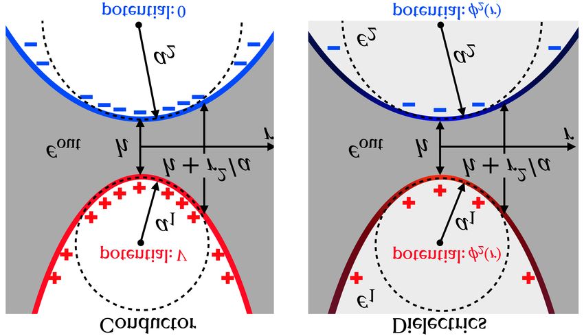
following boundary integral equation,                                                                                   ●
                                                                                                             ●
                                                                                                             ●●
                                                                                                              ●
                                                                                                              ●●
                                                                                                               ●●
                                                                                                                ●●
                                                                                                                 ●●
    1 + ǫr                                      1 − ǫr                                                             ●●
           σb + (1 − ǫr )ǫout (Eb + Ef ) · n̂ =        σf .     (11)
      2                                           2                                                                     ●
                                                                                                                             ●    ●
Above, the electric field strength at the surface due to in-
duced bound charge σb and free charges σf are expressed as                                                              ●
surface integrals (α = b, f),                                                                                ●
                                                                                                             ●●
                                                                                                              ●
                                                                                                              ●●
                                                                                                               ●●
                       1                  r − r′                                                                ●●●
                              ˆ
             Eα =                 dS ′              σα (r′ ).   (12)                                               ●●   ●         ●
                     4πǫout              |r − r′ |3

By our convention, the surface normal n̂ points outward.
For clusters of multiple particles, it is understood that dif-
ferent particles may have different values of permittivity ǫr .            Figure 3: Electrostatic energy of a pair of identical spheres.
Equation (11) is linear in σb and σf . After discretization, the           (a) and (b): asymmetric charge Q = (q, −q). (c) and
bound charge is obtained by inverting the coefficient array.               (d): symmetric charge Q = (q, q). In (b) and (d), dots
The apparent divergent diagonal entries while discretizing                 are numerical results obtained using our proposed method,
the surface integral eq. (12) can be re-parameterized to re-               and curves are exact prediction obtained using the tangent-
produce the correct self-energy. Further numerical details                 sphere coordinate (SI).
can be found in ref. 8. In all calculations by BEM presented
in this work (the dimer example used the exact series ex-
pansion. 10 ), we meshed each spherical surface into 17342                     For the asymmetric case, interfacial polarization en-
triangular patches such that mesh size is about 0.03 a.                    hances the inter-particle attraction. To illustrate this effect,
    In general, for a cluster of n particles, n separate nu-               we subtract the energy of two isolated spheres from that of
merical calculations with n independent charge vectors Q                   a dimer, then plot it against the gap distance in Fig. 3, for
are needed to determine the full capacitance matrix C. The                 three representative values of ǫr : 10, 102 and 104 . In ab-
computational cost can be reduced by imposing the sym-                     sence of the polarization effect, the energy curves would ex-
metry of the cluster configuration. Subtracting from C the                 hibit no dependence on ǫr , and appear flat over this narrow
singular contribution L̃ is expected to give the h-dependence              range of h/a values. As ǫr is increased from 1, we confirm
of the regular part H. However, unlike the conductor case,                 the expected, stronger distance dependence, as h → 0. In
where the coefficient to the logarithmic term is exactly                   particular, for the case of ǫr = 104 , an apparent logarithmic
known, the singular capacitance L̃ for dielectrics depends on              dependence on h is seen in Fig. 3a, which is precisely the
                                       (i)
the calculated contact potentials Ṽj , which is susceptible to            singularity revealed in eq. (7) and is stronger for higher per-
the numerical precision and what is meant by ‘contact point’               mittivity values. On the other hand, when the permittivity
on a surface mesh. In practice, we vary the gap distance h                 ǫr is decreased, this logarithmic dependence is cut off at an
and compute a few trial values of contact potentials, then                 increasingly larger separation and becomes almost invisible
select the one that ensures the difference Hij (h) = Cij − L̃ij            when ǫr = 10.
converges linearly with h as h → 0 for all the entries. In the                 The normalized energy difference, as shown in Fig. 3a,
following, three examples are presented to demonstrate the                 evaluated at h = 0, is show in Fig. 3b for different ǫr values.
nature of the contact singularity, and to show that the reg-               This contact energy represents the energy gain for bring-
ularization scheme allows us to obtain the energy of cluster               ing two particles from infinity to contact. In terms of the
of dielectric particles with small h.                                      normalizing energy unit, q 2 /(8πǫout a), its value is −1 with-
    The first example is a dimer of identical dielectric                   out the polarization effect, and becomes more negative as ǫr
spheres. It is the simplest example for demonstrating the                  increases, eventually reaching −2 at ǫr = ∞. 5 The con-
effects of interfacial polarization. 6,9,10,21 Except a study on           tribution from the polarization effect for ǫr & 100 is com-
the interaction between a conducting sphere and a dielec-                  parable to the coulombic attraction alone. Moreover, we
tric plane, 20 very few past work tried to evaluate the energy             notice a slow convergence of contact energy for permittiv-
at small separation, presumably due to the difficulty of re-               ities ǫr & 103 , owing to the weak ln ǫ2r dependence in the
solving the aforementioned contact singularity. Therefore,                 contact capacitance eq. (7) at h = 0. Finally, we affirm our
we analyzed the polarization effect for dielectric dimers in               results obtained from eq. (10), by comparing the contact en-
close contact, verified the singular behavior in eq. (7), and              ergies to the exact analytical results (SI).
showed that eq. (10) yields the full h-dependence of energy.                   For the symmetric case, the interfacial polarization
We studied both symmetric (Q = (q, q)) and asymmet-                        weakens the inter-particle repulsion, which is seen from the
ric (Q = (q, −q)) cases, for a range of permittivity values                h-dependence of dimer energy. However, by symmetry, the
(1 ≤ ǫr ≤ 106 ). The energy at h = 0 is presented as a func-               potential difference in the gap region vanishes and thus no
tion of relative permittivity, which agrees with the exact                 logarithmic behavior is observed in Fig. 3c. The energy
result (see SI) found using the tangent-sphere coordinate.                 scales linearly with h and a straightforward extrapolation

                                                                       5
gives the contact energy for all permittivity values plotted in
Fig. 3d. A much weaker polarization effect is found. Even for ●
the conductor case, only about 10% contact energy can be
●
attributed to polarization effects. The contact energies con- ● ●
verge for ǫr & 100, and reach 2(1/ ln 2 − 1) ≃ 0.88, in agree- ● ●
● ●
ment with Maxwell’s result 22 for the conducting dimers. As ●
for the asymmetric case, the full ǫr -dependence matches the
analytical calculation (SI). To conclude this example, we
note that the symmetric case is a peculiar example where ● ● ● ● ● ●
the contact singularity is strictly absent. For all other charge ●
ratios, using the decomposition in eq. (10) to isolate the
strong h-dependence is necessary.
The second example concerns the energy of 8 identical
spheres placed at the vertices of a cube, which illustrates
the importance of the second order contact for dielectric
◇
□
●
clusters. As discussed above, the singular capacitance L̃ □
◇
●
in eq. (10) contains not only contributions from the nearest □ ◇ □
● ◇
●
● □
◇
□ □
neighbors, but also those from the second-order and higher
◇ ◇
□
●
order neighbors. Therefore, a sphere at a vertex of a cube ◇◇ ◇ ◇
□
● ◇
forms a secondary contact with its 3 plane diagonal vertices, ● ●
and a third order contact with the body diagonal vertex. ●□
Even though the higher order contributions are minor, be- ●
cause at such large separation, these contacts cease to be ●
singular, keeping the second order contribution is essential
for obtaining the correct linear scaling of the regular capac-
itance with gap distance h shown in Fig. 4a.
As in the dimer case, these regularized capacitance al-
low us to evaluate the energy at arbitrarily small gap dis-
tance. Figure 4b shows the normalized energies when only
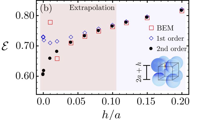
Figure 4: (a) Variation of entry H11 in the regular capac-
one particle is charged, for which all the energetic contribu-
itance array against separation. The results for the other
tions come from the interfacial polarization. Comparing the
entries are provided in Fig. S3. (b) Variation of electrostatic
results from BEM and our regularization schemes containing
energy against separation for dielectric spheres with ǫr = 100
varying order of contact contributions, it is clear that keep-
placed on cubic vertices, where one sphere is charged.
ing the higher order singular contribution is necessary for
correctly evaluating the energy for h/a . 0.05. In contrast,
no such terms are needed for the conducting case. chosen. For the string packing, we considered two extreme
The third example is our main result on the energy of placings: at one end (string-1) and in the middle (string-2).
clusters, from which the cohesive energy is obtained by sub- For each particle configuration and charge assignment, we
tracting the self-energy of particles at infinite separation. considered two scenarios: charge transfer between contact-
We considered two limiting configurations: the most ex- ing particles is permitted (Fig. 5a) and prohibited (Fig. 5b).
tended one with all spheres arranged along a straight line When inter-particle charge transfer is permitted, while
(string), and the most compact one with all spheres posited maintaining uniform charge distribution on each individual
at the vertices of the platonic solids (polyhedron). In our particle, the energy E can be calculated using Q · C−1 · Q/2.
earlier work on the conducting spheres, the charges are al- Minimizing this energy subject to the constraint of constant
lowed to flow freely between contacting spheres. The energy total charge q, the optimal charge assignment is found to
of polyhedron packing is found to be lower than that of the be Qe = q C · u/Ce , where u ≡ (1, 1, · · · , 1) and Ce ≡
n
string packing at a finite separation. However, as the gap
P
i,j=1 Cij . This implies that the optimal charge Qe pro-
distance decreases, the polarization effects due to contact duces identical average surface potentials for all the parti-
singularity become increasingly relevant, which ultimately cles, which generalizes the ‘equipotential’ concept for con-
makes the string packing to be energetically more favor- ductors. 5 Correspondingly, the minimized energy is given
able than the polyhedron packing. For the dielectric cases, by q 2 /(2Ce ), where the mean capacitance Ce weakly de-
we show that the weakened contact singularity causes an- pends on the dielectric permittivity. In this scenario, there
other crossover between the relative stability of string-like is no need to differentiate string-1 and string-2 configura-
and polyhedral packings. tions. The energies of string and polyhedron configurations
As the previous example, to highlight the polarization at h = 0 are plotted in Fig. 5a, for ǫr = 10 and 500. For
effects, a unit charge q is placed on one sphere. For sym- all configurations, the energy decreases with the cluster size
metric polyhedron packing, this charged sphere is arbitrarily n monotonically since the redistributed surface charges are
62 is lower than that of string-1 for identical n, because the
charged particles in the middle of the string can polarize the
particles in two half strings. Further, the energies for both
string-1 and string-2 configurations saturate as the cluster
size grows beyond n = 12, because the polarization effect is
short-ranged. To assess the relative stability of compact or
extended configurations, we then only need to focus on the
string-2 and the polyhedron cases.
Our results indicate that the relative energetic stability
depends on the permittivity. For ǫr = 10, the energy of
the polyhedron packing is lower than the string-2 packing,
which is opposite to the characteristic result for conductors
shown in Fig. 5a. Therefore, we expect a crossover from
stable compact packing to stable open packing at interme-
diate permittivity values. This is indeed the case shown
for ǫr = 500, whereby the energies of compact and open
○ □ configurations closely trace each other, and the relative en-
□ ergetic stability changes at n = 4 and n = 8 respectively.
□
○ ○ As ǫr is further increased, the energy curves of correspond-
□
○
ing configuration will converge to those in Fig. 5a, reversing
○○□
□ ○○○○○○○○○ ○ the relative stability of open and compact packings.
□ □ In summary, we generalized our previous work on con-
○
□○
○ □ ducting particles, 5 and developed a scheme to resolve the
○○□○○○○○ singular contact charges between touching dielectric spheres,
○
□ which regularizes the full capacitance array by isolating the
□ singular contributions, i.e., eq. (10). Using this scheme, we
obtain the cohesive energies for dielectric clusters at zero
separation containing up to n = 20 particles, which is dif-
ficult to resolve with brutal force numerical calculations.
Our results show that the shape of stable clusters formed
Figure 5: Size dependence of electrostatic energy E for from dielectric particles depends on the permittivity ratio
string-like and polyhedral configurations, with fixed to- ǫ : open clusters is more stable for large ǫ , and compact
r r
tal charge. (a) Charge transfer is permitted. Dashed clusters is more stable for small ǫ . Our scheme is applica-
1/3 r
curve: E = (2/n) /(2 ln 2), the energy for polyhedral ble to systems with arbitrary packing geometry, charge dis-
configurations of conducting spheres. 5 Solid curve: E = tribution, and containing asymmetric interfaces that have
ln(2na/r0 )/[n ln 2 ln(2a/r0 )], the energy for a conducting different permittivities and radii of curvature on the con-
cylinder of the same volume with length L = 2na and radius tacting particles. At the heart of our scheme is the contact
r0 = 0.816 a. 23 (b) Charge transfer is prohibited. The total singularity, which resembles those encountered in the study
charge q resides on the middle particle of the string (string- of thermal conduction 16 and momentum transport across a
2) and an arbitrary vertex of polyhedron (polyhedron). narrow gap. 24
further apart. The dependence on permittivity is surpris- References
ingly weak, and the size-dependence is nearly indistinguish-
able from that of the conductor case. 5 Two curves are ob- [1] J. Kolehmainen, A. Ozel, Y. Gu, T. Shinbrot, and
tained by treating the cluster as a single conductor respec- S. Sundaresan. Phys. Rev. Lett., 121:124503, 2018.
tively, whose capacitance scales with the length scale of the
cluster, i.e., n1/3 for the polyhedron packing and n/ ln(n) [2] V. Lee, S. R. Waitukaitis, M. Z. Miskin, and H. M.
for the string packing. 5 The extended string packing has Jaeger. Nature Phys., 11:733, 2015.
a lower cohesive energy because its effective capacitance is [3] E. V. Shevchenko, D. V. Talapin, N. A. Kotov,
higher than that of the compact polyhedron packing. S. O’Brien, and C. B. Murray. Nature, 439:55, 2006.
More interesting behavior is found (Fig. 5b) when charge
transfer is prohibited. The dependence on permittivity is ev- [4] J. W. Merrill, S. K. Sainis, and E. R. Dufresne. Phys.
ident for all three cases: string-1, string-2, and polyhedron. Rev. Lett., 103:138301, 2009.
To better visualize energies of string-2 and polyhedron pack-
[5] J. Qin, N. W. Krapf, and T. A. Witten. Phys. Rev. E,
ing, energies of string-1 is presented in Fig. S4) The energy
93:022603, 2016.
is lower for the cluster with higher permittivity, because
the polarization effect is stronger. The energy of string- [6] A. Russell. P. R. Soc. Lond. A-Conta., 82:524, 1909.
7[7] J. Lekner. P. Roy. Soc. A-Math. Phy., 468:2829, 2012.
[8] K. Barros, D. Sinkovits, and E. Luijten. J. Chem.
Phys., 140:064903, 2014.
[9] E. B. Lindgren, A. J. Stace, E. Polack, Y. Maday,
B. Stamm, and E. Besley. J. Comput. Phys., 371:712,
2018.
[10] H. Lian and J. Qin. Mol. Syst. Des. Eng., 3:197, 2018.
[11] J. Qin, J. J de Pablo, and K. F. Freed. J. Chem. Phys.,
145:124903, 2016.
[12] M. Shen, H. Li, and M. O. De La Cruz. Phys. Rev.
Lett., 119:138002, 2017.
[13] K. Barros and E. Luijten. Phys. Rev. Lett., 113:017801,
2014.
[14] Z. M. Sherman, D. Ghosh, and J. W Swan. Langmuir,
34:7117, 2018.
[15] L. G. Leal. Advanced Transport Phenomena: Fluid Me-
chanics and Convective transport Processes. Cambridge
University Press, 2007.
[16] G. K. Batchelor and R. W. O’Brien. P. Roy. Soc. A-
Math. Phy., 355:313, 1977.
[17] O. D. Kellogg. Foundations of Potential Theory.
Courier Corporation, 1953.
[18] X. Jiang, J. Li, X. Zhao, J. Qin, D. Karpeev,
J. Hernandez-Ortiz, J. J. de Pablo, and O. Heinonen.
J. Chem. Phys., 145:064307, 2016.
[19] L. Poladian. Q. J. Mech. Appl. Math., 41:395, 1988.
[20] S. V. Kalinin, E. Karapetian, and M. Kachanov. Phys.
Rev. B, 70:184101, 2004.
[21] J. D. Love. Q. J. Mech. Appl. Math., 28:449, 1975.
[22] J. C. Maxwell. A Treatise on Electricity and Mag-
netism. Oxford: Clarendon Press, 1873.
[23] J. D. Jackson. Classical Electrodynamics. John Wiley
& Sons, 1999.
[24] R. H. Davis, J. A. Schonberg, and J. M. Rallison. Phys.
Fluids. A-Fluid., 1:77, 1989.
8Exact polarization energy for clusters of contacting dielectrics
Supplementary information
Huada Lian1 and Jian Qin2,*
1
Department of Materials Science & Engineering, Stanford University
arXiv:2104.04175v1 [cond-mat.soft] 9 Apr 2021
2
Department of Chemical Engineering, Stanford University
*
Corresponding author: jianq@stanford.edu
April 12, 2021
We provide a detailed derivation of a spectral method for the electrostatic problem of two touching dielectric spheres
carrying uniform free surface charges in the tangent-sphere coordinates. The similar problem of touching dielectric spheres
in presence of an electrostatic field has been solved by Pitkonen previously. 1 We begin by introducing the tangent-sphere
coordinates and review some useful mathematical facts about the Poisson’s equation in the tangent-sphere coordinates.
We then provide a step-by-step derivation of the theory and illustrations of the method at the end.
First, we introduce the notation of the tangent-sphere coordinates by defining the transformation from the tangent-
sphere coordinates (µ, ν, ϕ) to the Cartesian coordinates (x, y, z)
µ cos ϕ µ sin ϕ ν
x= , y= , z= . (1)
µ2 + ν 2 µ2 + ν 2 µ2 + ν 2
where z-axis is the line connecting centers of two spheres. In this curvilinear coordinate, 2 spherical surfaces tangent to
xy-plane at the origin have constant ν value in ν ∈ (−∞, +∞). The value of ν is determined by the radius of the spherical
surface through ν = ±1/(2a), where + and − indicate the surfaces with z > 0 and z < 0, respectively. ν = 0 denotes the
xy-plane thereby. The surface of a circular toroid centered at origin without a hole, whose radius of circular section is µ,
has a constant µ value in µ ∈ [0, +∞). Lastly, ϕ ∈ [0, 2π] is the azimuth angle. The Euclidean distance d between points
(µ, ν, ϕ) and (µ′ , ν ′ , ϕ′ ) is expressed as
1/2
µ2 − 2µµ′ cos(ϕ − ϕ′ ) + µ′2 + (ν − ν ′ )2
d= (2)
(µ2 + ν 2 )(µ′2 + ν ′2 )
The electrostatic potential φ is governed by the Poisson’s equation ∇ · ǫ(r)∇φ(r) = −ρf (r)/ǫ0 , where ǫ(r) and ǫ0 are
the relative permittivity and the vacuum permittivity, and ρf (r) is the free charge distribution. ρf (r) is nonzero only if r is
on the surfaces in our problem setting. We denote φi (i = 1, 2) as the potential inside the sphere i and φ0 as the potential
outside two spheres. Within each region, the potential φi satisfies the Laplace’s equation ∇2 φi = 0 and then the solution
φi can be deduced from the general solution of Laplace’s equation in tangent-sphere coordinates by matching the values
of φi on boundaries.
The potential function φ(µ, ν, ϕ) satisfying the Laplace’s equation in the tangent-sphere coordinates is R−separable 2 ,
in which R(µ, ν) ≡ (µ2 + ν 2 )1/2 , and has the following general form
( )
cos nϕ
ˆ ∞
λν −λν
φ(µ,ν, ϕ) = R(µ, ν) dλ λJn (λµ) An (λ)e + Bn (λ)e . (3)
0 sin nϕ
Above, n takes nonnegative integrers n = 0, 1, 2, . . ., Jn (x) is the n-th order Bessel function of the first kind. An (λ), Bn (λ)
are two continuous spectra of λ that will be determined through matching boundary values. The integral above is the
Hankel transform of order n. The definition of Hankel transform of order n and its inverse transform are
ˆ ∞
Φn (µ, ν) = dλ λJn (λµ)Φn (λ, ν), (4a)
0
ˆ ∞
Φn (λ, ν) = dµ µJn (λµ)Φn (µ, ν). (4b)
0
1Owing to the rotational symmetry of the dimer problem we concerned, we shall only need the solution with n = 0 and thus
the ϕ-dependence can be dropped in our discussion below. We refer the further details about tangent-sphere coordinates
to ref. 2
We present below a step-by-step derivation of the spectral method for the case of asymmetric free charges Q = (q, −q).
The other case of symmetric free charge Q = (q, q) is dealt in the identical procedure, whose final form of solution would
be provided directly in parallel with that of the asymmetric case. To simplify the algebra, we consider the dimer of
identical spheres with radius a1 = a2 = a = 12 and define the permittivity contrast ǫr = ǫin /ǫout , where ǫin and ǫout are
the relative permittivities of the particles and the medium. The vacuum permittivity ǫ0 is set to the unity in below. The
surfaces of two spheres then have the constant value ν = ±1 in our convention and the centers of sphere are (0, ±2, 0) in
the tangent-sphere coordinates. For convenience, the potentials φ and energies E shown below are always normalized by
the self potential and self energy of a single isolated sphere in the vacuum, i.e. q/(4πǫ0 a) and q 2 /(8πǫ0 a), respectively.
For the dimer with asymmetric free charges, the potential has to be antisymmetric with respect to the xy-plane, i.e.
φ(µ, ν) = −φ(µ, −ν). Therefore, we only need to consider the potential φ1 and φ0 in the upper half space ν > 0. The
potentials outside the sphere φ0 and inside the sphere φ1 are
(µ2 + ν 2 )1/2 (µ2 + ν 2 )1/2
1 1
φ0 (µ, ν) = − 2 + ψ0 (µ, ν),
ǫout (µ2 + (ν − 2)2 )1/2 (µ + (ν + 2)2 )1/2 ǫout
(5)
(µ2 + ν 2 )1/2
1 1
φ1 (µ, ν) = 1− 2 + ψ1 (µ, ν).
ǫout (µ + (ν + 2)2 )1/2 ǫout
Here, the first part of contribution in the parenthesises come from the free charges of two spheres. The second part,
potentials ψ0 and ψ1 , represents the contribution from the induced bound charges. One can show that the first part
satisfies the Laplace’s equation by themselves alone, which follows that the ψ0 and ψ1 do the same.
The potentials ψ0 and ψ1 generated by the induced bound charges can then be expressed in the form of eq. (3)
ˆ ∞
ψ0 (µ, ν) = R(µ, ν) dλ λJ0 (λµ) 2A(0) (λ) sinh λν , (6a)
ˆ0 ∞
ψ1 (µ, ν) = R(µ, ν) dλ λJ0 (λµ) B (1) (λ)e−λν . (6b)
0
The superscript ‘(i)’ of the spectra A(0) (λ) and B (1) (λ) denotes the region to which they belong. Outside the sphere,
ψ0 (µ, ν) is an odd function with respect to ν so that we have ψ0 (µ, ν) = −ψ0 (µ, −ν) and consequently A(0) (λ) = −B (0) (λ)
resulting in eq. (6a). Inside the sphere, ψ1 (µ, ν) is finite everywhere including ν = +∞ (ν → +∞ denotes the smallest
spherical surface, which approaches the Cartesian origin within the sphere 1.) Therefore, A(1) (λ) = 0 is necessary to
keep the eλν from blowing up the integrand. Now, our object is to find the spectra A(0) (λ) and B (1) (λ) that match the
boundary values of φ0 and φ1 on the interface ν = 1.
Two spectra A(0) (λ) and B (1) (λ) are determined by the two boundary conditions on ν = 1: (a) the continuity of
potential across the boundary and (b) the discontinuity of normal component of electric field across the boundary, which
equals to the free surface charge density required by Gauss’s law. Mathematically, we have
φ0 (µ, 1− ) = φ1 (µ, 1+ ) (7a)
∂φ0 ∂φ1 1
−(µ2 + ν 2 ) +ǫr (µ2 + ν 2 ) = . (7b)
∂ν ν=1− ∂ν ν=1+ a
The normal component of electric field on the surface ν is |E| = −(µ2 + ν 2 ) ∂φ ∂ν , pointing inward (outward) on ν = 1
(ν = −1).
To obtain the equations for the spectra, we manipulate eq. (7a) and eq. (7b) in following steps: (1) Inserting eq. (5); (2)
Dividing both sides by (µ2 + 1)1/2 ; (3) Applying Hankel transformation of the zeroth order to both sides. Equation (7a)
is then transformed to
2A(0) (λ) sinh λ = B (1) (λ)e−λ ≡ C(λ) (8a)
where C(λ) is an auxiliary function defined for convenience. With eq. (8a), two unknown spectra are effectively reduced
to one. The normal boundary condition eq. (7b) is proceeded in the same way but dividing both sides by (µ2 + 1)3/2 . In
terms of C(λ), it becomes
ˆ ∞
µJ0 (λµ) ∞
ˆ ∞
(ǫr + coth λ) µJ0 (λµ)
ˆ
dµ 2 dτ τ J0 (τ µ)C(τ ) − λC(λ) = dµ 2 − (e−3λ + 2e−λ ). (8b)
0 µ +1 0 ǫr − 1 0 (µ + 1)(µ2 + 9)1/2
2Two useful Hankel transformations needed in our manipulation here are
ˆ ∞
ν
µ 2 J (λµ)dµ = e−λν /λ,
2 )1/2 0
(9a)
0 (µ + ν
ˆ ∞
ν
µ 2 J0 (λµ)dµ = e−λν . (9b)
0 (µ + ν 2 )3/2
The integral involving two Bessel functions J0 on LHS of eq. (8b) can be simplified by integrating over µ first. The
formula 6.541 in ref. 3 provides us a clean result to it
ˆ ∞ (
µJ0 (λµ)J0 (τ µ) I0 (λ)K0 (τ ), λ ≤ τ,
dµ 2+1
= (10)
0 µ I0 (τ )K0 (λ), λ > τ.
where I(x) and K(x) are modified Bessel functions of the first kind and second kind, respectively. On the RHS of eq. (8b),
the integral can be simplied by inserting the inverse Hankel transform of (µ2 + 9)−1/2 utlizing the eq. (9a) and changig
the order of integration
ˆ ∞ ˆ ∞ ˆ ∞
µJ0 (λµ) −3τ µJ0 (λµ)J0 (τ µ)
dµ 2 = dτ e dµ . (11)
0
2
(µ + 1)(µ + 9) 1/2
0 0 µ2 + 1
The inner integral can be evaluated in terms of the modified bessel functions again by eq. (10).
For future convenience, we define a new auxiliary function g(λ)
ǫr + coth λ
g(λ) ≡ λC(λ). (12)
ǫr − 1
Combining with the above simplifications on the integrals, the integral equation of C(λ) eq. (8b) is eventually reduced to
an integral equation of g(λ)
λ ∞
ǫr − 1 ǫr − 1
ˆ ˆ
g(λ) − K0 (λ) dτ I0 (τ ) g(τ ) − e−3τ − I0 (λ) dτ K0 (τ ) g(τ ) − e−3τ = (e−3λ + 2e−λ )
0 ǫr + coth τ λ ǫr + coth τ
(13)
The integral equation of g(λ) above is a Fredholm integral equation of the second kind. It can be solved by transforming
it to an differential equatino of g(λ) after differentiating eq. (13) with respect to λ twice. The first differentiation is carried
out in the following steps: (1) Dividing both sides by K0 (λ); (2) Differentiating both sides with respect to λ; (3) multiplying
both sides by λK02 (λ). Equation˜(13) becomes
ˆ ∞
ǫr − 1
λ(K0 (λ)g ′ (λ) + K1 (λ)g(λ)) − dτ K0 (τ ) g(τ ) − e−3τ = λ[−(3e−3λ + 2e−λ )K0 + (e−3λ + 2e−λ )K1 ]
λ ǫr + coth τ
(13.1)
′
′ 2 I0
The recurrence relation K0 (λ) = K1 (λ) and also the equivalence K0 K0 = 1/λ have been used.
Another direct differentiation with respect to λ of eq. (13.1) will get rid of the integral by Lebniz integral rule and lead
to an ODE of g(λ) for asymmetric free charges Q = (q, −q)
ǫr − 1
(λg ′ )′ + − λ g(λ) = (−2 + 8λ)e−3λ ,
ǫr + coth λ (14)
′
g (0) = −5, g(∞) = 0,
where another recurrence relation K1′ (λ) = −K0 (λ) − K1 (λ)/λ has been used and two boundary conditions are derived
through examining the behavior of g(λ) for λ = 0 and λ → ∞. Differentiating eq. (13) with respect to λ and evaluating
it at the limit λ → 0 will simply leave us with g ′ (0) = −5 as the derivatives of two integral expression with respect to λ
in eq. (13) vanish at λ = 0. On the other hand, g(∞) = 0 is necessary to ensure the integrability of eq. (3) when µ = 0.
Following the same procedure, we can derive another ODE of g(λ) and boundary conditions for the case of symmetric free
charge Q = (q, q). Here, we save the repetitive algebra and simply present its final result
ǫr − 1
(λg ′ )′ + − λ g(λ) = −(−2 + 8λ)e−3λ ,
ǫr + tanh λ (15)
′
g (0) = 5, g(∞) = 0.
3The major difference from eq. (14) is that the hyperbolic cotangent function in the denominator becomes the hyperbolic
tangent function, reflecting the even symmetry of potential about the xy-plane. The solutions of g(λ) for both cases with
several representative values of ǫr are presented in Fig. (S1). P
The contact energy that we are looking for is simply E = 12 i=1,2 Qi Vi in our problem setting, where Vi is the mean
surface potential of sphere i. For spheres, the mean surface potential can be represented by the potential evaluated at
its center due to the spherical symmetry. Therefore, we only need the potentials at (0, ±2, 0) for the contact energies
E = 12 Q1 φ1 (0, 2, 0) + 21 Q2 φ2 (0, −2, 0), in which φi is calculated by eq. (3) with spectra found by solving respective ODE
of g(λ). The contact energies for the dimer of identical spheres are presented for both cases of symmetric charges and
asymmetric charges with ǫr ranging from 0 to ∞ in Fig. (S2). The spectral method generalizes to dimer of spheres with
different radii and permittivities immediately, and more importantly, to spheres with higher order multipole charges.
References
[1] M. Pitkonen. Polarizability of a pair of touching dielectric spheres. J. Appl. Phys., 103(10):104910, 2008.
[2] P. Moon and D. E. Spencer. Field Theory Handbook: including coordinate systems, differential equations and their
solutions. Springer, 2012.
[3] I. Solomonovich G. and I. Moiseevich R. Table of Integrals, Series, and Products. Academic press, 2014.
4Supplementary figures
Figure S1: The solutions of g(λ) for both cases of asymmetric charges and symmetric charges with several representative
values of ǫr are presented. The solutions converge slowly in the asymmetric case due to the ln ǫ2r dependence of singular
contact charges shown in the main text. On the other hand, the ones converge fast in the symmetric case. The solutions
of ǫr = 10 and ǫr = 102 are almost indistinguishable for the case of symmetric charges.
5●
●
Figure S2: The electrostatic energy of a touching pair of identical spheres for the case of asymmetric charges and symmetric
charges. To emphasize the role of the electrostatic interaction, the energy of two isolated spheres, Eself is subtracted from
the total energy E. At ǫr = 1, the polarization effect vanishes and thus the interaction is simply the coulombic interaction
between two touching spehres, i.e. −1 and 1, in the unit q 2 /(8πǫ0 a). When ǫr > 1, the polarization effect enhances the
attraction and makes the interaction energy approach −2 at the conducting limit ǫr → ∞. For the symmetric case, the
interaction energy quickly converges to the known result, 2/ ln 2 − 2 ≈ 0.88. When ǫr < 1, the polarization effect screens
the coulombic interaction for both cases, which reduces the interaction energy to 0 at about ǫr ≈ 10−2 .
6●
● ●
●
●
●
●
●
●
● ● ● ● ● ● ● ●
●
● ●
● ● ● ● ● ● ● ●
●
● ● ● ● ● ● ● ● ●
● ● ● ● ● ● ● ● ●
Figure S3: The regular part Hij of capacitance coefficient Cij as a function of the normalized gap distance h/a. The
indices of spheres are denoted in the sketch of the cube configuration. With respect to the sphere 1, sphere 2 is one of
the nearest neighbor, sphere 5 is on one of the plane-diagonal vertices, and sphere 8 is on the body-diagonal vertex. The
nonlinear behavior of Cij gradually diminishes for the pair of spheres forming only a secondary contact.
○ △ □
□
△
○ ○ △ □
□
△
○○○○○○○○○○○ ○
○ △△
△
□ □ △ △△ △△ △△ △ △
○○ □ □
△□ ○ ○ ○ ○ ○ ○ ○ □
○ ○
△
△△△△
□ △△ △△ △
□ □
Figure S4: Size dependence of electrostatic energy E for string-like and polyhedron packing with fixed total charge, when
charge transfer is prohibited. The total charge q resides on one end of the string (string-1), the middle particle of the
string (string-2), and an arbitrary vertex of polyhedron (polyhedron).
7You can also read