Flux reconstruction for the NIR camera CAGIRE at the focus of the Colibr ı telescope
←
→
Page content transcription
If your browser does not render page correctly, please read the page content below
Flux reconstruction for the NIR camera CAGIRE at the
                                                               focus of the Colibrı́ telescope
                                              Alix Nouvel de la Flèchea , Jean-Luc Atteiaa , Hervé Valentina , Marie Larrieua , Jérémie Boya ,
                                              Olivier Gravrandb , Olivier Bouladec , Jean-Claude Clemensd , Aurélia Secround , Eric Kajfaszd ,
                                              Olivier Llidod , Stéphane Basae , François Dolone , Johan Floriote , Simona Lombardoe , Adrien
                                               Lamouref , Laurent Rubaldof , Bruno Fiequef , Julien Roumegouxf , Hervé Geoffrayg , Alan M.
                                                                      Watsonh , William H. Leeh , and Nathaniel Butleri
arXiv:2209.00386v1 [astro-ph.IM] 1 Sep 2022

                                                            a
                                                            IRAP, Université de Toulouse, CNRS, CNES, UPS, (Toulouse), France
                                                               b
                                                                 CEA-LETI, 17 Avenue des Martyrs, 38054, Grenoble, France
                                                                    c
                                                                      CEA-IRFU,Orme des Merisiers, Gif-sur-Yvette, France
                                                               d
                                                                 Aix Marseille Univ, CNRS/IN2P3, CPPM, Marseille, France
                                                                 e
                                                                   Aix Marseille Univ, CNRS, CNES, LAM, Marseille, France
                                                                    f
                                                                      LYNRED, 364 Av. de Valence, Veurey-Voroize, France
                                                                        g
                                                                          CNES, 18 Av. Edouard Belin, Toulouse, France
                                               h
                                                 Instituto de Astronomı́a, Universidad Nacional Autónoma de México, Apdo Postal 70-264,
                                                                              Cd. Universitaria, CDMX, México
                                                i
                                                  School of Earth and Space Exploration, Arizona State University, Tempe AZ 85287, USA

                                                                                                ABSTRACT
                                              CAGIRE is the near infrared camera of the Colibrı́ robotic telescope, designed for the follow-up of SVOM alerts,
                                              mainly Gamma Ray Bursts (GRBs), and the quick imaging of sky regions where transient sources are detected
                                              by the SVOM satellite. CAGIRE is based on the Astronomical Large Format Array (ALFA) 2k x 2k SWIR
                                              sensor from the French consortium CEA-LYNRED. In the context of CAGIRE the sensor is operated in “Up the
                                              Ramp” mode to observe the sky in a square field of view of 21.7 arcmin on a side, in the range of wavelengths
                                              from 1.1 to 1.8 µm. An observation with CAGIRE consists of a series of short (1-2 minutes) exposures during
                                              which the pixels are read out every 1.3 second, continuously accumulating charges proportionally to the received
                                              flux, building a ramp.
                                                  The main challenge is to quickly process and analyse these ramps, in order to identify and study the near
                                              infrared counterparts of the bursts, within 5 minutes of the reception of an alert. Our preprocessing, which is
                                              under development, aims at providing reliable flux maps for the astronomy pipeline. It is based on a sequence
                                              of operations. First, calibration maps are used to identify saturated pixels, and for each pixel, the usable
                                              (non saturated) range of the ramp. Then, the ramps are corrected for the electronic common mode noise,
                                              and differential ramps are constructed. Finally, the flux is calculated from the differential ramps, using a
                                              previously calibrated map of pixel non-linearities. We present here the sequence of operations performed by
                                              the preprocessing, which are based on previous calibrations of the sensor response. These operations lead to
                                              the production of a flux map corrected from cosmic-rays hits, a map depicting the quality of the fit, a map
                                              of saturated pixels and a map of pixels hit by cosmic-rays, before the acquisition of the next ramp. These
                                              maps will be used by the astronomy pipeline to quickly extract the scientific results of the observations, like the
                                              identification of uncatalogued or quickly variable sources that could be GRB afterglows.
                                                 Further author information: (Send correspondence to Alix Nouvel de la Flèche)
                                                 Alix Nouvel de la Flèche: E-mail: alix.nouvel-de-la-fleche@irap.omp.eu
                                                 Jean-Luc Atteia: E-mail: Jean-Luc.Atteia@irap.omp.eu
1. INTRODUCTION
The SVOM mission (Space based multi-band astronomy Variable Objects Monitor ) aims at observing transient
high energy sources, such as gamma ray bursts (GRBs).1 One goal of this Sino-French mission is the study of the
origin and environment of GRBs, and their use as tools to study the infancy and the evolution of the universe and
its first stars. The mission is designed to combine a space and a ground segment and to make the most of their
synergy. Based on the localization of the bursts detected by ECLAIRs onboard SVOM, the ground-based robotic
telescope Colibrı́, operating from the Observatorio Astronómico Nacional in San Pedro Mártir, will quickly point
the source and acquire images of the burst error box at near infrared (NIR) and visible wavelengths.2 The
presence of a burst appears in the images as a new unidentified star, often with rapid luminosity variations,
justifying the need for a telescope able to point the source in less than 30 s. Moreover the visible camera does
not allow to detect high redshift candidates (z ≥ 7.4), and the near infrared domain is needed to detect, monitor
and study them. To do so, a near infrared camera, CAGIRE (CApturing Grbs InfraRed Emission), has been
developed.
In this paper we describe the hereafter called preprocessing pipeline, used to reconstruct the flux received by
the detector of CAGIRE, from the ramps acquired. The preprocessing pipeline has been tested on ramps taken
with the RATIR instrument.3
2. CAGIRE OPERATION
2.1 Presentation of the camera
CAGIRE is a scientific camera sensitive in the near infrared between 1.1 and 1.8 µm, located at one of the
Nasmyth foci of the robotic telescope Colibrı́.2 When Colibrı́ receives a burst alert, it quickly points the source
and CAGIRE acquires images of the sky in the NIR domain, within a square field of view of 21.7 arcmin on a
side, to cover the error boxes of ECLAIRs.4 CAGIRE acquisitions will start soon after the telescope pointing
and consist of a series of short (1-2 minutes) exposures, processed right after their acquisition, in order to identify
potential afterglows within 5 minutes of the reception of an alert.
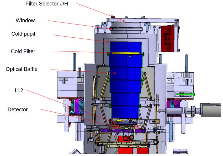
The camera is composed of three subsystems: a cryostat housing the detector which is maintained at a
constant temperature of 100K, a close electronics on the telescope, mounted on the structure supporting the
instruments, and a remote electronics located in the control room. The light arriving from the telescope is
focused on the detector by a series of lenses in a warm optical bench. At the entrance of the cryostat it crosses a
warm filter allowing to select the desired photometric channel (J or H). Then, it enters the cryostat and crosses a
cold filter cutting all the wavelengths longer than 1.8 µm, and a re-imaging cold lens, before reaching the detector
(fig 1).
Figure 1. Model of the CAGIRE cameraThe detector is read in science mode with 32 outputs at the readout frequency of 100 kHz, such that the whole
array is read every 1.3 s. It will be used in up-the-ramp mode, in which the pixels continuously accumulates
charges, roughly proportionally to the flux received by the camera during the exposure. Pixels are read every
1.3 s, creating a ramp of the accumulated signal, for each pixel. This mode allows to fulfill the requirement of
having a temporal resolution better than 2 s. The exposures will last from one to two minutes, in order to keep the
sky background below few tens of percent of the sensor’s dynamic range. This non-destructive acquisition mode
enables more flexibility to process the data after their acquisition, and doesn’t lead to data rate issues because
of the localization of the telescope on ground. The sky resolution of the system is of 0.64 arcsec/pixel. This
resolution implies that the detector will receive a flux from the sky background of about 150 electrons/pixel/s
for the J photometric channel and about 1250 electrons/pixel/s for the H channel.
2.2 The ALFA sensor
The camera CAGIRE is equipped with an Astronomical Large Format Array (ALFA) detector of 2048 by 2048
square pixels of 15 µm on a side, manufactured by the French company LYNRED, and based on the MCT
(Mercury Cadmium Telluride) technology developed at CEA-LETI.5 The detector covers a spectral range from
0.8 µm to 2.1 µm,6 justifying the need for a blocking filter for wavelengths longer than 1.8 µm on CAGIRE. The
detection layer in HgCdTe (MCT) is hybridized with indium bumps on a Read Out Integration Circuit (ROIC),
designed and manufactured by LYNRED. The array is composed of 2040 by 2040 active pixels surrounded by a
ring of pixels under permanent reset. Around them, reference pixels, with the same electronics as the active ones
but not sensitive to light, can be used for Read-Out Integrated Circuit (ROIC) noise reduction. The detector is
read through 32 outputs simultaneously. More information about the detector is given in Fieque et al. 2018.5
In order not to saturate the detector with the sky background, and to let enough dynamic available for bright
objects, the exposures have to be shorter than 200 s in the J band and shorter than 30-60 s in the H band. This
leads to accumulate around 30,000 electrons from the sky background (∼ 14 of the potential well capacity), with
Poisson statistical fluctuations of approximately 170 electrons rms per pixels. This is significantly larger than
the readout noise, which is not a critical parameter for CAGIRE.
The data under study in this article have been provided by CEA-IRFU for ramps acquired with the ALFA
sensor, and by CPPM for data acquired with the ROIC.
2.3 Data processing
One of the advantages of CAGIRE is to be located on the ground, allowing full ramps to be stored and exploited
to measure the flux received by the detector. Ideally, the signal, measured in Analog to Digital Units (ADU),
should be proportional to the integrated flux, and the flux should correspond to the slope of the ramp.
However, the data are impacted by several effects due to the detector or the environment (see section 3),
requiring a pre-processing of the data before their analysis by the astronomy pipeline. Among the detector effects,
conversion gain inhomogeneities (per pixel and per channel), readout noise, small fluctuations of bias voltages
and pixel non-linearities affect the measure of the flux. Some non-operational pixels can also give erroneous
values. Among environmental effects, cosmic-ray hits have a huge impact on the flux measurement and need to
be taken into account. As CAGIRE aims at identifying quickly the NIR counterparts of high-energy transients,
the ramps must be processed “on-the-fly”, implying that one ramp must be processed before the next arrives to
avoid data clogging. For this purpose, we have developed a fast and robust pre-processing pipeline, described in
the next section.
3. PREPROCESSING PIPELINE
When CAGIRE acquires a ramp, it is necessary to quickly provide a reliable map of the flux to the astronomy
pipeline. The preprocessing aims at constructing such maps, cleaned from instrumental effects. It is composed of
several steps summarized in table 1, and some of them require calibration maps, which are described in section
5. At some point, treatments depend on the number of frames in the ramp, as described in sections 3.2 and 3.3.
The last step, the measurement of the flux, requires differential ramps. A differential ramp is constructed by
subtracting 2 consecutive frames of the ramp. It is equivalent to the ramp derivative. This process is detailed in
section 4.3.1 Identification of saturated pixels
The first step is the identification of saturated pixels and the construction of a map of saturated pixels at the
end of a ramp. This is necessary because saturation can lead to persistence, lasting for minutes to hours after
the illumination.7
In order to identify saturated pixels, we compare the flux of the last frame of the ramp with the calibrated
map of the saturation level. Pixels reaching the saturation level are flagged as saturated. The map of saturated
pixels is an important piece of information, because the saturation during an acquisition can impact the following
acquisitions as saturated pixels are likely to show some persistence. This persistence can leave a detectable signal
even in the absence of illumination. The map of saturated pixels thus allows to avoid confusing a GRB afterglow
with the persistence of a previously saturated star. Even if saturation is not the only cause of persistence, the
list of saturated pixels is an important piece of information for the correct interpretation of sources detected by
the astronomy pipeline. Figure 2 shows the ramp of a saturating pixel.
Figure 2. Example of a saturating pixel
3.2 Single frame ramps
In some special cases (e.g. focus adjustment with bright sources), it may be useful to acquire ramps containing a
single frame. In such cases the preprocessing consists of two steps: the subtraction of the electronics bias and the
correction of the ROIC common mode noise using the reference pixels. This second step is described in section
3.3.1.
3.3 Ramps with N ≥ frames
If the ramp is composed of 2 frames or more, the preprocessing involves the following steps (table 1): the
correction of the common noise using the reference pixels, the construction of a differential ramp for each pixel,
the identification and correction of pixels hit by cosmic-rays, and the fit of the differential ramp by a straight
line. These steps are described in some detail below.Step 1: Complete ramp headers
Ramp Update headers Raw ramp, with CAGIRE header
HK information
Step 2: Find saturated pixels
Last frame of raw ramp Find saturated pixels Map of saturated Pixels
Saturation Level map
Step 3: Subtract Master Bias and correct all frames with reference pixels
Raw ramp Subtract Master Bias and correct Ramp with corrected frames
Master Bias Map all frames with reference pixels
Step 4: Construct Corrected Differential Ramp
Corrected ramp Corrected differential ramp 1 (CDR1)
Step 5: Flag Cosmic Rays (CR) candidates
CDR 1 CR candidates Identification Map of CR candidates
(3 parameters) Corrected differential ramp 2 (CDR 2)
Step 6: Flux estimation
CDR 2 Flux estimation Flux and variance maps
Map of non-linearity coefficients (1 parameter)
Table 1. Pre-processing pipeline for ramps with N ≥ 2 frames. For each step, the left column gives the input parameters,
the middle column indicates the computation, and the right column the output. Files made available by the preprocessing
for the astronomy pipeline are shown in bold.
3.3.1 Correction with reference pixels
The pixel gain is very sensitive to small perturbations of the bias voltages, induced by the environment. Some
of these perturbations can be corrected when they affect several pixels in the same way. This is in particular the
case for perturbations impacting the column preamplifiers, which affect an entire channel. The noise generated
at channel level is often called common mode noise and it can be reduced thanks to sets of reference pixels
surrounding the matrix of active pixels. The reference pixels are identical to active pixels, except they are not
connected to the sensitive layer. Since they have the same electronics as active pixels, they are subject to the
same variations of the biases and temperatures as the active pixels. The aim is to correct the active pixels
from these variations, by subtracting a linear combination of the signals measured by nearby reference pixels, as
proposed by Bogna Kubik et al.8 for H2RG sensors. This correction is based on two steps. The first correction
is applied to a whole readout channel, and the second one to each row individually. First, we select the top andbottom reference pixels of a readout channel, representing 256 pixels, and we compute the mean of their values. Then, we subtract this mean to all the pixels of the channel, including the reference pixels themselves. Second, we select the left and right reference pixels of row L, plus 4 rows of reference pixels above and below row L, 9 rows in total, representing 54 pixels. We subtract their mean to row L. This second correction is computed with the left and right reference pixels previously corrected by the first correction. This method allows a reduction of the readout noise by ∼ 25% and is applied to each frame of the ramp. This correction also corrects the offset, channel by channel, if it was not subtracted beforehand. As we are computing our flux with differential ramps, constructed from the subtraction of two consecutive frames, this offset correction has no impact on our process. Figure 3 highlights the impact of the correction on the uniformity of a frame. However, the bias has not been subtracted beforehand here, hence, the main visible effect is an offset correction. Figure 3. Example of a frame before correction by reference pixels[left] and after correction by reference pixels [right]. The axes correspond to the pixel number on the detectors, and the color bars are in ADU. In this example, the bias has not been subtracted, hence, the main visible effect is an offset correction. 3.3.2 Working with differential ramps As explained before, the ALFA sensor used in this study has a non-destructive readout. The signal continuously builds up in the pixels and it is read out every 1.3 s, making ramps whose slope is proportional to the flux received by the pixel. Instead of fitting the ramps, which integrate the signal, we have chosen to fit the differential ramps constructed by subtracting the signal measured in frame k-1 to the signal measured in frame k. While the information contained in the differential ramps is equivalent to the one contained in the ramps, the differential ramps presents the advantage of being a series of independent measurements of about the same value, allowing a more direct statistical interpretation of the results. Fitting the differential ramps also requires one less parameter. Figure 4. Experimental ramp (blue point), linear extrapolation of the beginning of the ramp (orange) and saturation level (dashed red line) [left]. Differential ramp (blue points) and its fit (orange line) [right]
Figure 4 gives an example of a ramp and the corresponding differential ramp. The left panel of figure 4 shows
a measured ramp (blue points) and the associated linear extrapolation of the beginning of the ramp (orange).
The right panel shows the differential ramp constructed from the left curve.

3.3.3 Identification and correction of pixels impacted by cosmics-rays
Cosmic rays are high energy particles coming from outer space. They generate high-energy secondary particles
in the atmosphere of the Earth, which can leave a track in the detector, especially for observatories located at
high altitudes. Even if few cosmic-ray hits are detected on the calibration maps measured in the laboratory, a
larger number of pixels will be impacted by comic-rays during observations. To avoid errors on the flux map,
cosmic-rays hits have to be localized. We discuss here a method allowing to localize them and to recover the
flux of pixels impacted by cosmic-rays. Cosmic-ray impacts have a particular signature on the ramps and on the
differential ramps, by creating a big jump between the signal measured in two consecutive frames. This jump
is responsible for a high variance on the differential ramp. However, erratic pixels, or pixels impacted by high
fluxes can also show differential ramps with a high variance. To differentiate a pixel hit by a cosmic-ray from a
pixel illuminated by a bright source, we rely on the ratio R of the variance over the mean of the differential ramp.
For bright stars, this ratio should be small because of the large mean. On the contrary, this ratio will be large
for pixels impacted by cosmic-rays and erratic pixels. Pixels with both the variance and R exceeding predefined
limits (constructed from their respective histograms), have probably been impacted by cosmic-rays. Once these
pixels are selected, their differential ramps are tested individually. We compute the Median Absolute Deviation
(MAD) of the differential ramp, and we define a limit to localize points very different from the median signal.
This limit is plotted with a full row on the figure 5 [left]. It is defined by:

                                       madLim = Signalmedian + X × M AD

    Where ”X” is a configuration parameter that will be defined with data acquired with the camera in its final
configuration. If we detect a point of the differential ramp with a value larger than madLim, it is probable that
a cosmic-ray impinged it, hence we suppress this point from the differential ramp of the pixel, and thus avoid
to consider it in the calculation of the flux. To differentiate them from erratic pixels, cosmic-rays impacts are
identified only if a single point exceeds the limit madLim. If no point is detected above madLim, or several
points are detected above madLim, the pixel is an erratic one, and it is rejected from the list of comic-rays hits.

Figure 5. Differential ramp of a pixel impacted by a cosmic-ray at frame number k=18, and limit to identify cosmic-rays.
[left]. Ramp of a pixel impacted by a cosmic-ray at frame number k=18, and its fit before (orange) and after (green)
correction [right].

    Thanks to this method, we can detect cosmic-rays hits and recover the flux of the impacted pixels (Fig 5,
right). The preprocessing pipeline returns the localization of the identified comic-rays hits, and the flux corrected
from the impact of these cosmic-rays.
3.3.4 Flux measurement on the differential ramp
This is the most important work of the preprocessing, but also the longest if it is not optimized. It relies on the
fit of differential ramps, and it is described in section 4.
3.4 Products of the preprocessing pipeline
The following maps are returned by the pipeline:
• The position of saturated pixels.
• The position of pixels impacted by cosmic-rays.
• The number of frames used to fit the differential ramp of each pixel (section 4.3).
• The signal received by each pixel as described in section 4.4.
• The error on the signal as described in section 4.4.
3.5 Performances of the preprocessing pipeline
In terms of performances, we measured the time necessary to perform each step of the pipeline for the whole
array, depending of the number of frames in the ramp, see table 2. The pipeline has been written in Python, and
is implemented in a laptop with a microprocessor Intel Core i7-10810U @ 1.10GHz. The performances should
thus be accelerated in the final process, thanks to the use of Julia language and a more powerful processor.
Number of frames considered 7 20 46 90
Exposure duration [s] 9 27 60 120
Finding saturated pixels [s] 0.008 0.008 0.008 0.02
Computing the limit of the fit [s] 0.3 0.7 2 6
Correction by reference pixels [s] 0.8 2.3 5 9.7
Creation of the differential ramp [s] 0.2 0.8 2.0 3.6
Computing output variables (Flux, Error, Cosmic-rays hits)[s] 1.5 2.5 5.6 19.4
Duration of the preprocessing 6 9 18 54
Table 2. Table of the characteristic processing time of the pipeline over the 4 millions of pixels
Table 2 demonstrates that, even with this configuration, the processing time is systematically shorter than
the duration of the acquisition, which allows to finish the process before starting a new acquisition, as required.
4. MEASURING THE FLUX IN NEAR-REAL TIME
While the flux received by a pixel is encoded in the slope of its ramp, many factors can perturb its measure.
First, the slope of the ramp decreases slowly due to the fact that the charges accumulated during an exposure
tend to increase the effective capacitance of the pixel. Second, minute changes of the bias voltages produce
slight variations of the gain, and consequently of the slope. Third, cosmic-rays may hit one or several pixels,
producing a large number of charges and a jump in the ramp of these pixels. Finally, the sensor’s non uniform
illumination during sky exposures adds supplementary difficulties, like saturated pixels. Due to the wide field of
view of CAGIRE, there will be many tens of saturated stars in standard exposures. It is nevertheless possible to
get a correct estimate of the flux on these pixels, at the condition of measuring the slope of the ramp with only
the frames recorded before saturation. It is thus necessary to evaluate, for each pixel, the range of frames to be
used for the evaluation of the flux.
We have discussed the management of saturation, gain changes and cosmic-ray hits in the previous section,
so this section is specifically dedicated to the management of non-linearities in the evaluation of the flux received
by a pixel.4.1 Dealing with non-linearities with differential ramps
The phenomenon of non-linearity can be seen in figure 4, where the signal on a pixel of an ALFA sensor shows
a slight deviation from linearity (measured ramp in blue, and linear signal in orange), which has to be taken
into account to estimate the flux from the ramp. Because of this deviation from linearity, the use of linear
regression over the ramp is not adapted to measure the flux. Moreover, the statistical uncertainty on the points
of the ramp increases with signal accumulation, because the detector noise is dominated by the photon Poisson
noise. To overcome this problem, we decided to work with the differential ramps, constructed as the difference
between two consecutive frames, as presented in the right panel of figure 4. At some point (frame number 90
approximately on figure 4), the ramp reaches a plateau (red dashed line), corresponding to the saturation level.
In the differential ramp, right panel, the saturation level corresponds to the sharp fall of the values. Close to
this saturation level, the deviation from linearity is higher, leading us to select a usable range of the ramp (linear
and non saturated) to evaluate the flux. The first step of our calibrations is the computation of the functional
form of the non-linearity function and the applicable range of this function. These two quantities are calibrated
thanks to calibration ramps under illumination provided by CEA-IRFU.
4.2 Calibration of pixels non-linearity
The choice of the fit of the differential ramps relies on the ability of the function to take the non-linearity into
account. The fits are computed on differential ramps. In order to choose, we compared three functions:
• A first order polynomial (a linear fit), where k is the frame number and the interesting parameter is a0 ,
the signal in ADU/frame, which is proportional to the incident flux. a1 is the non-linearity coefficient.
P1 (k) = a0 + a1 × k
• A second order polynomial (where the interesting parameter is a0 , the signal),
P2 (k) = a0 + a1 × k + a2 × k 2
• A non-polynomial function using a coefficient of non-linearity, defined by:
a0
Fδ (k) = 2
(1 − δ × a0 × k)
where a0 is the signal we are looking for, and δ the non-linearity coefficient.
As the goal of the preprocessing is to be precise on the estimation of the signal but also fast and robust, the
linear fit would be preferred. However, functions with more parameters could have the advantage of providing
more accurate fits. To compare the efficiency of these functions to fit our data, we compared the medians of
several quantities: the signal estimated by fitting a differential ramp, the variance on the fitted signal, the χ2
associated to the fits and the normalized χ2 associated to the fits. The normalized χ2 is computed by dividing
the χ2 value by the number of degrees of freedom of the function (number of points of the ramp fitted minus the
number of parameters of the fit, minus one). The results are computed on all the active pixels of the detector,
and the medians of these values over the detector are summarized in table 3. The three functions have been
used to fit the differential ramps over 80% of the dynamic range of the pixels.
Table 3 highlights values of the signal and of the χ2 that are very similar for the three functions, providing
no strong argument in favor of one function or another, from their sole capacity to fit the data. Looking at Table
3, we see that the median χ2 of the three functions, are very close, meaning that the 2nd order polynomial and
Fδ do not provide significant improvement, compared to the linear fit, which is the simplest function. We thus
decided to fit the differential ramps with a linear fit to compute the signal.
The a1 coefficient of the linear fit has units of f ADU
rame2 . It is the consequence of the increase of the effective
capacitance of the pixel while accumulating charges, which explains the deviation from linearity. We measured a
median value of this coefficient of -0.24 ADU/frame2 for active pixels. The negative sign reflects the capacitance
increase, and thus the decrease of the number of ADU encoded for the same number of charges received. The
role of this parameter in our process is described in section 4.3.Function 2nd order pol. 1st order pol. Fδ
Number of fitted parameters 3 2 2
Signal [ADU/frame] (median value) 193.5 193.3 193.5
Variance [ADU²/frame²] (median value) 7.4 3.1 3.4
χ2 (median value) 62.6 63.3 63.3
Normalized χ2 (median value) 0.947 0.942 0.927
Table 3. Comparison of the values of signal, variance, χ2 and normalized χ2 for the three non-linearity functions studied
here. The values are the median values over all the active pixels of the detector.
4.3 The fitting range of the ramps and the non-linearity coefficient
To determine the fitting range of the ramps, we worked with ramps provided by CEA-IRFU. These ramps have
been acquired with the detector under constant illumination during more than 4 min, to let the detector reach
saturation. We fit the differential ramps with a first order polynomial, and compute the signal as the zeroth
order parameter of the fit, called a0 . The first order parameter is called a1 and is representative of the loss of
signal between two consecutive frames caused by the non-linearity of the ramp. We then looked at the variations
of the estimated signal with the range of the ramp fitted, taken as a fraction of the saturation level. The results
are presented in Table 4 and show stable signal a0 estimates up to 80-90% of the saturation.
Saturation level fraction [%] signal [ADU/f] Error [ADU/f] Dev. from lin [%] Number of frames
10 % 193.255 4.9 0.3 10
20 % 193.164 3.5 0.9 18
30 % 193.135 3.0 1.5 27
40% 193.129 2.6 2.1 35
50 % 193.244 2.4 2.8 44
60% 193.358 2.4 3.4 53
70 % 193.350 2.3 4.0 62
80 % 193.234 2.4 4.7 71
90 % 193.214 2.6 5.3 80
Table 4. Signal estimation as a function of the maximum level of the ramp fitted, the associated error on the signal
coefficient and the deviation from linearity at this level. The last column represents the number of frames used to
compute the fit.
Figure 6. Histogram of the absolute value of the deviation from linearity at 80% of the saturation levelTable 4, highlights very stable signal coefficients with a fit by a first order polynomial, with variations smaller
than 0.1%. These results confirm our choice of using a first order polynomial to fit the differential ramps.
Moreover, we see that below 80% of the dynamic range, the deviation from linearity is smaller than 5% for most
pixels, which is not the case at 90% of the saturation. Figure 6 shows the histogram of deviation from linearity
for all active pixels at 80% of the dynamic range. It shows that pixels can have different behaviours. Because
of this dispersion better results are obtained when the fitting range is defined as a fraction of the saturation
level, instead of a deviation from linearity. If we choose a fitting range based on a given deviation from linearity
(e.g. 5%), for some very linear pixels the fitting range could exceed the saturation level, leading to an erroneous
value of the signal. We thus decided to fit the ramp until 80% of the saturation level to be sure to be in the
close-to-linear domain of the ramps.
Moreover, the fit of differential calibration ramps under illumination with a first order polynomial function
over 80% of the saturation range, allows us to construct a map of the non-linearity coefficient for each pixel
of the detector. However, the coefficients a0 and a1 are not “universal” as they depend on the illumination.
Specifically a0 depends on the signal, while a1 depends on the signal accumulated by the pixel. A way to get
rid of this dependence is to construct the parameter γ = aa12 , which can be shown to encode the non-linearity
0
intrinsic to each pixel (see Annex A). We thus use calibration ramps to construct a map of γ (figure 13 of annex
A). In the next section we discuss how this information is used to process ramps measured on the sky.
4.4 Measuring the signal with real ramps
The first step is to identify for each pixel, the frame number at which it reaches 80% of its saturation level, using
calibration maps described in section 5.1. This limit, labelled k80 is different for each pixel. The second step is
to compute the differential ramp and to estimate the signal, using a linear fit of the differential ramp.
dk = a0 + a1 × k (1)
For the stability of the signal estimate, we want to estimate only the signal a0 , considering the non-linearity as
a known parameter. Relying on the non-linearity parameter γ = aa21 , computed during the calibrations, equation
0
1 can be rewritten as follows.
dk = a0 + a20 × γ × k
where k is the number of the frame considered, a0 is the signal to be estimated, and γ, is the coefficient of
non-linearity described in the previous section. After some computation we find that the signal on sky data can
be computed by solving the equation:
A × a20 + B × a0 + C = 0
PN
where A = γ × (N2+1) ; B=1 and C = - N1 k=1 dk . N is the number of frames of the ramp used in the calculation.
In the end, we obtain the signal a0 in ADU/frame :
√
−B + B 2 − 4AC
a0 = (2)
2A
The error on this coefficient is defined by :
s
variance(dk )
Error(a0 ) =
N × (B 2 − 4AC)
The computation of a0 and its error are performed on the differential ramps up to k80 , for each pixel inde-
pendently. Figure 4, shows an example of a differential ramp (blue points) fitted by this method (orange line).
In this figure k80 = 81. More results on sky images are given in section 6.5. CALIBRATION MAPS
Calibration maps are created beforehand, in order to localize bad pixels (dead, erratic...), to measure the satura-
tion level, to construct the bias map and to evaluate the usable – sufficiently linear and unsaturated – range of the
ramp for each pixel. These calibration maps, which are necessary for the preprocessing pipeline, will be acquired
at the “Centre de Physique des Particules de Marseille” (CPPM) during the calibrations of the CAGIRE sensor.
5.1 The saturation level
First, a map of the saturation level per pixel is needed to evaluate the range of the ramp on which each pixel
can be operated. It is also a useful map to localize the pixels saturated during an acquisition. This map is
obtained by illuminating continuously the detector during the acquisition of a single ramp. The detector has to
be illuminated until saturation to compute the saturation level of each pixel. An example of a saturation map
acquired with the calibration data provided by CEA-IRFU is given figure 7.
5.2 Bias map
Before correcting the frames from the common mode noise, we need to subtract a Master Bias, measured during
calibration tests. A pseudo-bias is computed as the median signal of few tens of dark acquisitions of one frame.
This bias is required to deal with the first frame of a ramp. An example of a pseudo-bias map computed from 2
dark files provided by CEA-IRFU is given figure 7 [right].
Figure 7. Example of a saturation map. The saturation level is expressed in ADU. The bias has not been removed. [left].
Example of a bias map. [right]
5.3 Non-operational pixels
We also need a map of the non-operational pixels to avoid misidentifications. Pixels can be considered as non-
operational if they are dead or erratic. Hot pixels will be unusable only if they saturate in the very first frames of
the ramp. Cold pixels are problematic if their limited response to light introduces a signal very different from their
neighbours. Knowing their position can be useful for the astronomy pipeline. We explain in the next paragraphs
how we localize and characterize these pixels thanks to calibration maps in the dark and under illumination. In
the end, the map returned to the astronomy pipeline consists of a single map where all non-operable pixels are
flagged in the same way.
Hot pixels are pixels with an abnormally high signal in the dark. We notice that most of them are usable
while being illuminated. To find hot pixels, we compute the dark current, and we study pixels revealing a very
high dark current, or saturating pixels. Only saturating pixels and pixels with a dark current larger than to
2 electrons/s will be considered as unusable (see fig 8). These pixels represent less than 0.001% of the active
pixels. We also plotted here an ”operability” curve on the histogram, representing the fraction of events larger
than the value of x-axis. This curve highlights that very few pixels overcome the limit of 2 e-/s.Figure 8. Left: histogram of the dark current for a 60266 second long exposure and limit of hot pixels (green dashed line).
The red plot represents the ”operability” (the fraction of pixels with a dark current larger than the abscissa), which can
be read on the right vertical scale. Right: ramp of a hot pixel.
Cold pixels and dead pixels on the contrary, are pixels with an abnormally low response to light. To find
them, we compute the signal received by the detector while being illuminated by a constant flux, and we plot
the histogram of this signal. Pixels with a signal smaller than 500 electrons/s (see fig 9), are considered as cold
or dead. These pixels represent 0.11% of the active pixels. We also plotted here the cumulative distribution of
the histogram, representing the fraction of events smaller than the x-axis value. This curve highlights that very
few pixels are below the limit.
Figure 9. Left: histogram of the signal under illumination and the limit of dead and cold pixels (green dashed line). The
red plot represents the cumulative distribution (because the pixels of interest are below the histogram maximum), which
can be read on the right vertical scale. Right: ramp of a cold pixel (blue ramp) and ramp of an operable pixel (orange
ramp).
Erratic pixels are pixels with an unusual response to light, very dispersed, which can have different be-
haviours. To find them, we compute the variance of the signal, for each pixel. Erratic pixels are pixels with
a variance larger than 1000 electrons²/s²(fig 10). This limit is a preliminary result to define maps to test our
preprocessing pipeline. A study of these pixels with a response very different from a line is currently conducted
to better understand and localize them. With this limit of 1000 electrons²/s², erratic pixels represent 0.25% of
the active pixels. We also plotted here the ”operability” curve on the histograms, representing the fraction of
events larger than the value on the x-axis. This curve highlights the fact that very few pixels have an erratic
response, according to our definition.
In the end, very few pixels are considered as non-operational. They represent ' 0.35% of the active pixels.
Using them could produce false detections so that their localization has to be provided to the astronomy pipeline,
to avoid any misidentification based on the signal map.Figure 10. Left: Histogram of the variance on signal and limit of erratic pixels (green dashed line). The red plot represent
the operability, which can be read on the right vertical scale. Right: ramp of an erratic pixel
6. APPLICATION TO SKY IMAGES
In order to validate the preprocessing pipeline, we tested it on images of the sky acquired with RATIR. These
tests allow to confirm that the maps returned by the process are usable by the astronomy pipeline, but also to
ensure that the signal returned on known stars is in line with the one listed in catalogs like the 2MASS All-Sky
Catalog of Point Sources.9 It is also a way to test that the preprocessing works properly on ramps that are
dominated by the sky background, inhomogeneously illuminated and contaminated by cosmic-rays.
6.1 Pre-processing of RATIR images
The preprocessing pipeline described here has been tested on images of the sky taken with RATIR (the Reion-
ization And Transients InfraRed camera). RATIR is a multi-channel optical and near infrared imager operating
at the robotic 1.5-meter Johnson telescope at the Observatorio Astronómico Nacional in Mexico. This imager is
able to acquire images in the r,i,Z,Y,J and H bands simultaneously. It is composed of two H2RG detectors, of
2040 by 2040 active pixels, surrounded by 4 rows and lines of reference pixels.3 For the sake of testing CAGIRE’s
preprocessing, RATIR data have been acquired in up-the-ramp mode.
The mode of operation with RATIR is thus very similar to CAGIRE, and it is located at the same site. The
images acquired with RATIR are divided into two zones, one for the H photometric band and one for the J
photometric band. We process here the whole image but distinguish stars observed in the J channel and stars
observed in the H channel. Figure 11 represents the signal and the associated error computed for the H channel.
Figure 11. Example of a flux map and the associated error in the H channel
The data under study are composed of ramps of 30 frames, acquired every 1.45 s. We used these data to
compute the signal of ramps taken with RATIR, using CAGIRE’s preprocessing pipeline. We have to noticehere that we could not apply the steps of the preprocessing that use calibration maps. It means that we could
not compute the level at 80% of the saturation and all pixels are processed in the same way. Moreover pixels
saturating or non-operable pixels could not be removed. However we could apply the correction by reference
pixels and construct all the output maps except the map of saturated pixels. Despite this lack of calibration
maps, the process of ramps acquired with RATIR has not raised any particular issue. We are thus confident of
the robustness of the pre-processing. The following section is not part of the pre-processing pipeline but aims to
test the relevance of our outputs.
6.2 Results
After the pre-processing, we used the map of the signal, figure 11, to extract the sources with Source Extractor,10
and we cross-matched them with the catalog 2MASS All-Sky Catalog of Point Sources,9 thanks to Astrome-
try.net.11
Then, we compared the number of sources identified with the number of source detected, and the magnitude
measured by Source Extractor with the magnitude measured in the catalog 2MASS. The magnitudes esti-
mated by Source Extractor have been computed without reference to the zero magnitude of the instrument.
To make them comparable, we added an offset corresponding to the magnitude difference between 2MASS and
Source Extractor for the brightest star detected.
Number of extraction by Source Extractor 31
Number of extraction associated to 2MASS catalog 28
percentage of good extraction [%] 90.3
Table 5. Number of sources extracted in our map, number of extractions associated to 2MASS catalog and corresponding
percentage of good extractions.
We notice here 90.3% of good detection. However, the bad detections are located on a corner of the detector
presenting a ghost image, and could probably be avoided using the right calibration files.
Figure 12. Comparison of the magnitudes measured by source extractor with magnitudes in the 2MASS All-Sky Catalog
of Point Sources
The result plotted Figure 12 depicts the magnitude measured by Source Extractor versus the magnitude
of 2MASS catalog. Red and blue points are for J and H bands respectively. The magnitudes estimated arein line with 2MASS results. They are not intended to be accurate magnitudes, however, because they are
estimated with a single image, without correction of the sky background and with our very limited experience of
Source Extractor. The astronomy pipeline of CAGIRE will indeed provide much more accurate magnitudes.
Nevertheless, these first results show that the preprocessing fulfills its role, by providing images cleaned from
detector’s features and ready for the astronomical analysis, starting from realistic raw sky images. Finally,
CAGIRE is composed of pixels larger than RATIR’s, it has a larger field of view and uses a different sensor. The
preprocessing will thus need to be adapted to the sky images acquired by CAGIRE.
7. CONCLUSION AND PERSPECTIVES
We have discussed here a method to recover the sky signal, based on the fit of differential ramps, and its
integration into the preprocessing pipeline of CAGIRE. The pipeline has to be fast enough to process a ramp
before the acquisition of a new one. We have shown here that it fulfills these requirements, returning maps
usable by the astronomy pipeline, in a context of ramps dominated by the sky background. The input maps
of the pipeline (saturation, bias and non-operable pixels) and their acquisition have been described. We have
also presented the correction of the common mode noise thanks to a combination of the signal measured by
the reference pixels. Our method allows to recover the signal of pixels impacted by cosmic-rays, thanks to the
computation of the MAD of the differential ramp. A study of the speed performances of the pipeline has been
conducted to attest the compliance with the requirement for a fast processing. The data provided by this process,
were finally tested on sky images. We have shown that we are able to detect the objects with few errors and
to compute magnitudes in line with the ones from 2MASS catalog. For the future, we still need to study the
effects of persistence on a short time scale (∼ 1 minute, comparable to the duration of a ramp), particularly for
saturating pixels. To do so, we will base our work on the studies of T. Le Goff.7 The impact of persistence will
nevertheless be mitigated thanks to the use of a proper dithering strategy. Finally, our analyses, made with files
acquired at CEA-IRFU, confirm that the ALFA detector fulfills CAGIRE requirements, with a good linearity
and homogeneity, and very few defective pixels.
Acknowledgments
The calibration data used in the first parts of this paper were acquired at CEA by O. Boulade. The data has been
provided to IRAP in agreement with ESA. CAGIRE is partly funded by the French Centre National d’Etudes
Spatiales (CNES). The PhD contract of A. Nouvel de la Flèche is financed by CNES and LYNRED. This work
has been partially supported by the LabEx FOCUS ANR-11-LABX-0013.
The on sky data used in this paper were acquired with the RATIR instrument, funded by the University
of California and NASA Goddard Space Flight Center, and the 1.5-meter Harold L. Johnson telescope at the
Observatorio Astronómico Nacional on the Sierra de San Pedro Mártir, operated and maintained by the Ob-
servatorio Astronómico Nacional and the Instituto de Astronomı́a of the Universidad Nacional Autónoma de
México. Operations are partially funded by the Universidad Nacional Autónoma de México (DGAPA/PAPIIT
IG100414, IT102715, AG100317, IN109418, IG100820, and IN105921). We acknowledge the contribution of
Leonid Georgiev and Neil Gehrels to the development of RATIR.
REFERENCES
[1] J. Wei, B. Cordier, S. Antier, P. Antilogus, J. L. Atteia, A. Bajat, S. Basa, V. Beckmann, M. G. Bernardini,
S. Boissier, L. Bouchet, V. Burwitz, A. Claret, Z. G. Dai, F. Daigne, J. Deng, D. Dornic, H. Feng, T. Foglizzo,
H. Gao, N. Gehrels, O. Godet, A. Goldwurm, F. Gonzalez, L. Gosset, D. Götz, C. Gouiffes, F. Grise, A. Gros,
J. Guilet, X. Han, M. Huang, Y. F. Huang, M. Jouret, A. Klotz, O. La Marle, C. Lachaud, E. Le Floch,
W. Lee, N. Leroy, L. X. Li, S. C. Li, Z. Li, E. W. Liang, H. Lyu, K. Mercier, G. Migliori, R. Mochkovitch,
P. O’Brien, J. Osborne, J. Paul, E. Perinati, P. Petitjean, F. Piron, Y. Qiu, A. Rau, J. Rodriguez, S. Schanne,
N. Tanvir, E. Vangioni, S. Vergani, F. Y. Wang, J. Wang, X. G. Wang, X. Y. Wang, A. Watson, N. Webb,
J. J. Wei, R. Willingale, C. Wu, X. F. Wu, L. P. Xin, D. Xu, S. Yu, W. F. Yu, Y. W. Yu, B. Zhang, S. N.
Zhang, Y. Zhang, and X. L. Zhou, “The Deep and Transient Universe in the SVOM Era: New Challenges
and Opportunities - Scientific prospects of the SVOM mission,” arXiv e-prints , p. arXiv:1610.06892, Oct.
2016.[2] S. Basa and al., “COLIBRI, a 1.3m robotic telescope dedicated to the transient sky ,” in These proceedings,
SPIE.
[3] N. Butler, C. Klein, O. Fox, G. Lotkin, J. Bloom, J. X. Prochaska, E. Ramirez-Ruiz, J. A. de Diego,
L. Georgiev, J. González, W. H. Lee, M. G. Richer, C. Román, A. M. Watson, N. Gehrels, A. Kutyrev,
R. Bernstein, L. C. Alvarez, U. Ceseña, D. Clark, E. Colorado, A. Córdova, A. Farah, B. Garcı́a, G. Guisa,
J. Herrera, F. Lazo, E. López, E. Luna, B. Martı́nez, F. Murillo, J. M. Murillo, J. M. Núñez, M. H. Pedrayes,
F. Quirós, J. L. Ochoa, G. Sierra, H. Moseley, D. Rapchun, F. D. Robinson, M. V. Samuel, and L. M. Sparr,
“First light with RATIR: an automated 6 - band optical / NIR imaging camera,” in Ground-based and
Airborne Instrumentation for Astronomy IV, I. S. McLean, S. K. Ramsay, and H. Takami, eds., 8446,
pp. 336 – 342, International Society for Optics and Photonics, SPIE, 2012.
[4] O. Godet, G. Nasser, J.-. Atteia, B. Cordier, P. Mandrou, D. Barret, H. Triou, R. Pons, C. Amoros,
S. Bordon, O. Gevin, F. Gonzalez, D. Götz, A. Gros, B. Houret, C. Lachaud, K. Lacombe, W. Marty,
K. Mercier, D. Rambaud, P. Ramon, G. Rouaix, S. Schanne, and V. Waegebaert, “The x-/gamma-ray
camera ECLAIRs for the gamma-ray burst mission SVOM,” in Space Telescopes and Instrumentation 2014:
Ultraviolet to Gamma Ray, T. Takahashi, J.-W. A. den Herder, and M. Bautz, eds., 9144, pp. 625 – 639,
International Society for Optics and Photonics, SPIE, 2014.
[5] B. Fièque, A. Lamoure, F. Salvetti, S. Aufranc, O. Gravrand, G. Badano, O. Boulade, S. Mouzali, and
S. Basa, “Development of astronomy large focal plane array ”ALFA” at Sofradir and CEA,” in High Energy,
Optical, and Infrared Detectors for Astronomy VIII, A. D. Holland and J. Beletic, eds., 10709, pp. 33 – 51,
International Society for Optics and Photonics, SPIE, 2018.
[6] O. Gravrand, C. Lobre, J.-L. Santailler, T. Legoff, N. Baier, G. Badano, O. Boulade, T. Pichon, A. Nouvel-
Delaflèche, D. S. Giao, A. Maltere, S. Aufranc, F. Salvetti, J. Roumegoux, B. Brosse, and A. Lamoure,
“Fabrication and characterization of a high performance NIR 2kx2k MCT array at CEA and Lynred for
astronomy applications,” in Infrared Technology and Applications XLVIII, B. F. Andresen, G. F. Fulop, and
L. Zheng, eds., 12107, pp. 21 – 31, International Society for Optics and Photonics, SPIE, 2022.
[7] T. L. Goff, N. Baier, O. Gravrand, O. Boulade, and T. Pichon, “Persistence and dark current characterization
on HgCdTe short wave infrared imagers for astronomy at CEA and Lynred,” in X-Ray, Optical, and Infrared
Detectors for Astronomy IX, A. D. Holland and J. Beletic, eds., 11454, pp. 285 – 298, International Society
for Optics and Photonics, SPIE, 2020.
[8] B. Kubik, R. Barbier, A. Castera, E. Chabanat, S. Ferriol, and G. Smadja, “Impact of common modes
correlations and time sampling on the total noise of a H2RG near-IR detector,” in High Energy, Optical, and
Infrared Detectors for Astronomy VI, A. D. Holland and J. Beletic, eds., 9154, pp. 427 – 439, International
Society for Optics and Photonics, SPIE, 2014.
[9] R. M. Cutri, M. F. Skrutskie, S. van Dyk, C. A. Beichman, J. M. Carpenter, T. Chester, L. Cambresy,
T. Evans, J. Fowler, J. Gizis, E. Howard, J. Huchra, T. Jarrett, E. L. Kopan, J. D. Kirkpatrick, R. M. Light,
K. A. Marsh, H. McCallon, S. Schneider, R. Stiening, M. Sykes, M. Weinberg, W. A. Wheaton, S. Wheelock,
and N. Zacarias, “VizieR Online Data Catalog: 2MASS All-Sky Catalog of Point Sources (Cutri+ 2003),”
VizieR Online Data Catalog , p. II/246, June 2003.
[10] E. Bertin and S. Arnouts, “SExtractor: Software for source extraction.,” Astronomy and Astrophysics
Supplement 117, pp. 393–404, June 1996.
[11] D. L. D. W. H. K. M. M. Blanton and S. Roweis, “Astrometry.net: Blind astrometric calibration of arbitrary
astronomical images,” The Astronomical Journal 139(5), 2010.APPENDIX A. STABILITY OF THE NON-LINEARITY COEFFICIENT γ
We consider here a differential ramp characterized by the equation:
dk = A0 + A1 × k
We can define the signal value as:
k k
X X k(k + 1)
Sk = dj = A0 × k + A1 × dj = A0 × k + A1 ×
j=1 j=1
2
The non-linearity is defined by the relative deviation of Sk from the theoretical value, A0 × k :
Sk − A0 × k A1 (k + 1)
N on − Linearity(k) = = ×
A0 × k A0 2
If we do the same computation with a different signal A00 = x × A0 , we have :
A01 (k 0 + 1)
N on − Linearity 0 (k) = 0 ×
A0 2
Considering that, far from saturation level, the non-linearity is proportional to the accumulated signal Sk =
A0 × k, we have N on − Linearity = N on − Linearity 0 at the same accumulated signal level. We also have
A00 = x × A0 and k 0 = xk . We can then compute A01 :
N on − Linearity 0 (k) = N on − Linearity(k)
A01 × ( xk + 1) A1 × (k + 1)
=
A0 × 2x 2 × A0
k+1
A01 = x × A1 × k
x +1
k+1
We approximate the ratio : k ≈x
x +1
A00 2
A01 = x2 × A1 = A1 × ( )
A0
We can finally write:
A01 A1
= 2 =γ (3)
A02
0 A0
A1
We here conclude that the non-linearity coefficient γ defined by the ratio γ = A2 , is independent of the signal
0
received. Figure 13 shows the histogram of this coefficient computed with calibration data.Figure 13. Histogram of the γ coefficient, peaking around −6.5 10−6 .
You can also read