Global trends and European emissions of tetrafluoromethane (CF4), hexafluoroethane (C2F6) and octafluoropropane (C3F8)
←
→
Page content transcription
If your browser does not render page correctly, please read the page content below
Atmos. Chem. Phys., 21, 2149–2164, 2021
https://doi.org/10.5194/acp-21-2149-2021
© Author(s) 2021. This work is distributed under
the Creative Commons Attribution 4.0 License.

Global trends and European emissions of tetrafluoromethane (CF4),
hexafluoroethane (C2F6) and octafluoropropane (C3F8)
Daniel Say1 , Alistair J. Manning2 , Luke M. Western1 , Dickon Young1 , Adam Wisher1 , Matthew Rigby1 ,
Stefan Reimann3 , Martin K. Vollmer3 , Michela Maione4 , Jgor Arduini4 , Paul B. Krummel5 , Jens Mühle6 ,
Christina M. Harth6 , Brendan Evans1 , Ray F. Weiss6 , Ronald G. Prinn7 , and Simon O’Doherty1
1 Atmospheric   Chemistry Research Group, University of Bristol, Bristol, UK
2 Met  Office Hadley Centre, Exeter, UK
3 Empa, Swiss Federal Laboratories for Materials Science and Technology, Ueberlandstrasse 129,

Dübendorf, Switzerland
4 Department of Pure and Applied Sciences, University of Urbino, Urbino, Italy
5 Climate Science Centre, CSIRO Oceans and Atmosphere, Aspendale, Australia
6 Scripps Institution of Oceanography, University of California, San Diego, La Jolla, CA, USA
7 Center for Global Change Science, Massachusetts Institute of Technology, 77 Massachusetts Ave.,

Building 54-1312, Cambridge, MA, USA

Correspondence: Daniel Say (dan.say@bristol.ac.uk)

Received: 7 September 2020 – Discussion started: 15 September 2020
Revised: 18 December 2020 – Accepted: 1 January 2021 – Published: 12 February 2021

Abstract. Perfluorocarbons (PFCs) are amongst the most po-         0.007 ppt yr−1 until the early 1990s and then quickly grew
tent greenhouse gases listed under the United Nations Frame-       to a maximum of 0.03 ppt yr−1 in 2003–2004. Following a
work Convention on Climate Change (UNFCCC). With at-               period of decline until 2012 to 0.015 ppt yr−1 , the growth
mospheric lifetimes on the order of thousands to tens of           rate slowly increased again to ∼ 0.017 ppt yr−1 in 2019. We
thousands of years, PFC emissions represent a permanent            used an inverse modelling framework to infer PFC emis-
alteration to the global atmosphere on human timescales.           sions for northwest Europe. No statistically significant trend
While the industries responsible for the vast majority of these    in regional emissions was observed for any of the PFCs as-
emissions – aluminium smelting and semi-conductor man-             sessed. For CF4 , European emissions in early years were
ufacturing – have made efficiency improvements and intro-          linked predominantly to the aluminium industry. However,
duced abatement measures, the global mean mole fractions           we link large emissions in recent years to a chemical manu-
of three PFCs, namely tetrafluoromethane (CF4 , PFC-14),           facturer in northwest Italy. Emissions of C2 F6 are linked to
hexafluoroethane (C2 F6 , PFC-116) and octafluoropropane           a range of sources, including a semi-conductor manufacturer
(C3 F8 , PFC-218), continue to grow. In this study, we update      in Ireland and a cluster of smelters in Germany’s Ruhr val-
baseline growth rates using in situ high-frequency measure-        ley. In contrast, northwest European emissions of C3 F8 are
ments from the Advanced Global Atmospheric Gases Exper-            dominated by a single source in northwest England, raising
iment (AGAGE) and, using data from four European stations,         the possibility of using emissions from this site for a tracer
estimate PFC emissions for northwest Europe. The global            release experiment.
growth rate of CF4 decreased from 1.3 ppt yr−1 in 1979 to
0.6 ppt yr−1 around 2010 followed by a renewed steady in-
crease to 0.9 ppt yr−1 in 2019. For C2 F6 , the growth rate grew
to a maximum of 0.125 ppt yr−1 around 1999, followed by a
decline to a minimum of 0.075 ppt yr−1 in 2009, followed by
weak growth thereafter. The C3 F8 growth rate was around

Published by Copernicus Publications on behalf of the European Geosciences Union.

2150                                                               D. Say et al.: European emissions of CF4 , C2 F6 and C3 F8

1   Introduction                                                   abundant PFC in the atmosphere. The presence of C2 F6 has
                                                                   not been detected in the pre-industrial atmosphere (Trudinger
Perfluorocarbons (PFCs) – fully fluorinated hydrocarbons –         et al., 2016), and its sources are very similar to the anthro-
are a group of extremely potent greenhouse gases that are          pogenic sources of CF4 , with aluminium production and the
used extensively in the electronics and semi-conductor in-         semi-conductor industry accounting for approximately one-
dustry and are also emitted as a byproduct of aluminium and        third and two-thirds of the global budget in 2010, respec-
rare-earth metal smelting. As a consequence of their high          tively (Kim et al., 2014). C2 F6 is also a component of the
global warming potentials (GWPs), PFCs were listed under           refrigerant blend R-508 (50 %–70 % C2 F6 by weight, 30 %–
the Kyoto “basket”, a collection of gases for which regulation     50 % trifluoromethane (CHF3 ) by weight), which is used in
on their emissions was introduced under the Kyoto Proto-           very low temperature refrigeration, though this is thought to
col (UNFCCC, 2009). Countries listed under Annex 1 of the          be a minor source (Kim et al., 2014). Trudinger et al. (2016)
protocol are required to report annual PFC emissions to the        reported peak global emissions of ∼ 3.6 Gg yr−1 in 2000,
United Nations Framework Convention on Climate Change              which was followed by a decline until 2010 and stabilisation
(UNFCCC).                                                          thereafter (Engel and Rigby, 2019).
   Tetrafluoromethane (CF4 , PFC-14) is the simplest and              Octafluoropropane (C3 F8 , PFC-218) has an atmospheric
most abundant PFC in the atmosphere, with a reported global        lifetime of 2600 years and a GWP100 of 7000 (Burkholder
mean background mole fraction of 82.7 pmol mol−1 (dry-air          et al., 2019). It is the fourth most abundant PFC, after perflu-
mole fraction in parts per trillion; ppt) in 2016 (Prinn et al.,   orocyclobutane (PFC-318, c-C4 F8 ; see Mühle et al., 2019),
2018). CF4 has a GWP of 6500 over a 100-year time hori-            with a global mean mole fraction of 0.63 ppt in 2016 (Prinn
zon (GWP100 ) (Burkholder et al., 2019) and, with an es-           et al., 2018). The Emission Database for Global Atmospheric
timated atmospheric lifetime of 50 000 years (Burkholder           Research v4 (EDGAR, 2009) attributes C3 F8 emissions to
et al., 2019), it is the longest-lived greenhouse gas known.       refrigeration/air-conditioning use and semi-conductor manu-
Background atmospheric mole fractions of CF4 have risen            facture. While the aluminium industry is not thought to be a
sharply since the beginning of the industrial revolution. How-     major source, low concentrations of C3 F8 have been detected
ever, unlike other PFCs, which are solely anthropogenic in         from smelter stacks (Fraser et al., 2003). At present, the alu-
origin, CF4 is also emitted naturally from calcium fluorites       minium industry does not account for C3 F8 in their emis-
(CaF2 ) present in continental crust (Trudinger et al., 2016).     sions reporting, and its low concentration means that it may
Harnisch and Eisenhauer (1998) estimated that the fluorite         not even be detectable by the instruments employed by the
reservoir is sufficient to maintain an atmospheric background      industry to monitor PFC emissions (Trudinger et al., 2016).
mole fraction of approximately 40 ppt. More recently, this            As a result of their exceedingly long lifetimes, PFC emis-
was refined to 34.05 ± 0.33 ppt (Trudinger et al., 2016).          sions represent a permanent (on human timescales) alteration
   The predominant anthropogenic source of CF4 to the              to the atmosphere. PFC sinks are dominated by decomposi-
atmosphere is primary aluminium production. Kim et al.             tion during high temperature combustion (Cicerone, 1979;
(2014) estimated that aluminium smelting accounted for             Ravishankara et al., 1993; Morris et al., 1995). Both alu-
∼ 68 % of global emissions in 2010. Emissions from the             minium and semi-conductor industries have targeted PFCs
smelting of aluminium ore occur predominantly during “an-          for emissions reductions in an effort to curb greenhouse gas
ode effects”, when the feed of alumina to the cell is restricted   emissions (Trudinger et al., 2016).
resulting in formation of CF4 but also during routine opera-          In this study, we present atmospheric PFC measurements
tion (Wong et al., 2015). CF4 is also used commercially in the     from the Advanced Global Atmospheric Gases Experiment
semi-conductor industry as an etchant gas for plasma etching       (AGAGE) network. These data are used to update baseline
and as a cleaning agent in chemical vapour deposition (CVD)        mole fraction data and growth rates. The atmospheric mea-
tool chambers. In recent years, the smelting of rare-earth         surements from European stations are used, in conjunction
metals, such as neodymium, has also been cited as a small but      with an inverse modelling framework, to estimate PFC emis-
growing source of CF4 (Cai et al., 2018; Zhang et al., 2018).      sions for northwest Europe. We compare our emissions maps
Firn air measurements show that the atmospheric abundance          to the European Pollutant Release and Transfer Register (E-
of CF4 has increased rapidly since 1960 (Trudinger et al.,         PRTR), which contains a record of PFC emissions from in-
2016). While emissions peaked in 1980 and have since de-           dustrial facilities. Finally, we explore potential of using one
clined, Engel and Rigby (2019) report renewed growth in re-        such PFC-emitting facility as a release location for a tracer
cent years.                                                        experiment.
   Hexafluoroethane (C2 F6 , PFC-116) has an atmospheric
lifetime of 10 000 years and a GWP100 of 9200 (Burkholder
et al., 2019), making it the most potent PFC, and fourth most
potent greenhouse gas, listed under the Kyoto basket in terms
of its GWP100 . With a global mean background mole fraction
of 4.56 ppt in 2016 (Prinn et al., 2018), it is the second most

Atmos. Chem. Phys., 21, 2149–2164, 2021                                              https://doi.org/10.5194/acp-21-2149-2021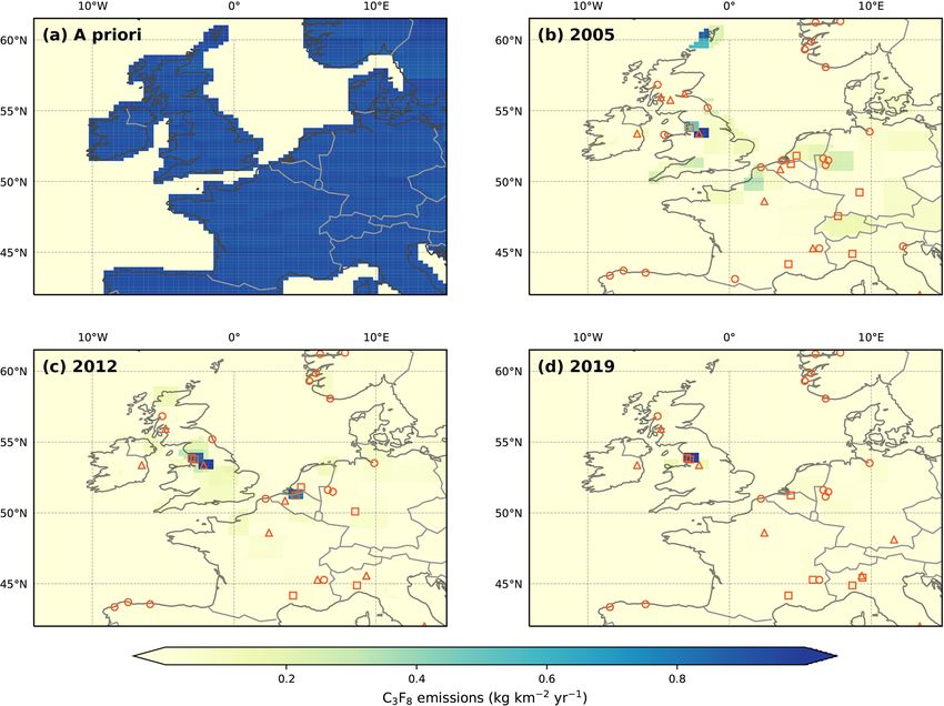
D. Say et al.: European emissions of CF4 , C2 F6 and C3 F8                                                                          2151

Figure 1. Average footprint emission sensitivity in picoseconds per
mole (ps mol−1 ) obtained from NAME 30 d backward calculations
for the four measurement sites – Mace Head (MHD), Tacolneston
(TAC), Jungfraujoch (JFJ) and Mt. Cimone (CMN) – during 2015.
Measurement sites are marked as red triangles.
                                                                      Figure 2. Modelled semi-hemispheric monthly average CF4 mole
                                                                      fractions (30–90◦ N: blue; 0–30◦ N: green; 30–0◦ S: purple; 90–
2     Materials and methods                                           30◦ S: red). Monthly averaged baseline observations are shown as
                                                                      data points with 1σ error bars. The more sparse filled circles rep-
                                                                      resent northern (blue) and southern (red) hemispheric air archive
2.1    Instrumentation                                                samples. The solid trend lines were calculated using the AGAGE
                                                                      12-box model with emissions from the inversion as input. The lower
Long-term in situ PFC measurements were made by the                   plot shows the model-derived mole fraction growth rate, smoothed
AGAGE (Prinn et al., 2018) network. With the exception                with an approximate 1-year filter, for each semi-hemisphere (dashed
of Monte Cimone (CMN), all stations were equipped with                lines) and the global mean with 1σ uncertainty (solid line and shad-
a Medusa pre-concentration system coupled with a gas chro-            ing).
matograph (GC, Agilent) and quadrupole mass selective de-
tector (MSD) (Miller et al., 2008). At CMN, measurements
of C3 F8 (neither CF4 or C2 F6 were measured) were made               charge ratio (m/z) of 69, and m/z 50 was used as a quali-
using an in-line auto sampler and pre-concentration device            fier. C2 F6 was monitored on m/z 119 with a qualifier ion of
coupled to a GC mass spectrometer (Maione et al., 2013).              m/z 69, and C3 F8 was monitored on m/z 169 with m/z 119
Observations from the five “core” AGAGE stations – Mace               as a qualifier. For each gas, the ratio of target to qualify-
Head (MHD), Ireland; Trinidad Head (THD), USA; Ragged                 ing ion was continuously monitored to ensure that co-eluting
Point (RPB), Barbados; Cape Matatula (SMO), American                  species did not interfere with the analysis. Weekly system
Samoa; and Cape Grim (CGO), Tasmania – were used to                   blanks were conducted to test for system leaks and/or car-
infer global trends. Observations from MHD; Jungfraujoch              rier gas impurities. MHD and TAC showed small blanks for
(JFJ), Switzerland; Tacolneston (TAC), United Kingdom;                all three PFCs. These were carefully assessed for each car-
and CMN, Italy were used to infer northwest European emis-            rier gas cylinder. Where the blank variability was negligible,
sions (Fig. 1). Station details are given in Table 1.                 all measurements made using that cylinder were blank cor-
   Each air measurement was bracketed by analysis of a                rected. Measurements coinciding with high and/or variable
working (quaternary) standard to account for short-term               blanks were rejected.
drifts in detector sensitivity. At JFJ and TAC, every two air
measurements were bracketed. Quaternary standards were                2.2   Archived air samples
linked to a set of primary calibration scales – SIO-05 for
CF4 and SIO-07 for C2 F6 and C3 F8 – via a hierarchy of               The atmospheric histories of CF4 , C2 F6 and C3 F8 were ex-
compressed real-air standards held in 34 L internally electro-        tended backwards in time via analysis of northern and south-
polished stainless-steel canisters (Essex Industries, Missouri,       ern hemispheric archived air samples (Figs.2–4). A full de-
USA). The estimated absolute accuracy of the calibration              scription of the collection and analysis of these samples can
scales is ∼ 1.5 %, ∼ 2 % and ∼ 4 % for CF4 , C2 F6 and C3 F8 ,        be found in Mühle et al. (2010) and Trudinger et al. (2016).
respectively. Average measurement precisions, estimated as            In short, northern hemispheric archive samples, which were
the standard deviation of the bracketing standards for all sites      provided by a range of laboratories, were filled under base-
across all years, were estimated to be ∼ 0.18 %, ∼ 0.77 % and         line conditions using a range of filling techniques and for
∼ 2.70 % for CF4 , C2 F6 and C3 F8 , respectively. Mass spec-         different purposes. The southern hemisphere archive samples
trometers were run in selective ion mode (SIM). CF4 was               are part of the Cape Grim air archive (CGAA; Fraser et al.,
detected on its base (most abundant) ion, with a mass over            2003) and were cryogenically filled into electro-polished

https://doi.org/10.5194/acp-21-2149-2021                                                Atmos. Chem. Phys., 21, 2149–2164, 2021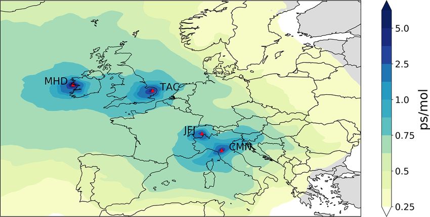
2152                                                                                    D. Say et al.: European emissions of CF4 , C2 F6 and C3 F8

Table 1. Station names, locations and inlet heights for the instruments used to quantify global and regional PFC emissions. Note that for the
mountain site, JFJ, the inlet is situated below the instrument.

                 Site name              Acronym          Location               Altitude (m a.s.l.)        Inlet (m a.g.l.)      Data range
                 Cape Grim              CGO              41◦ S, 145◦ E                            94                    10       Jan 2004–present
                 Cape Matatula          SMO              14◦ S, 171◦ W                            82                    10       May 2006–present
                 Jungfraujoch           JFJ              47◦ N, 8◦ E                            3580                  −15a       Apr 2008–present
                 Mace Head              MHD              53◦ N, 10◦ W                              8                    10       Dec 2003–present
                 Monte Cimone           CMN              44◦ N, 11◦ E                           2165                    10       Jan 2008–present
                 Ragged Point           RPB              13◦ N, 59◦ W                             32                    10       May 2005–present
                 Tacolneston            TAC              53◦ N, 1◦ E                              56                  185b       Aug 2012–present
                 Trinidad Head          THD              41◦ N, 124◦ W                           107                    10       Apr 2005–present
               a The original JFJ inlet was situated at 10 m a.g.l. The instrument began sampling from the −15 m a.g.l. inlet on 15 August 2012. b The
               original TAC inlet was situated at 100 m a.g.l. The instrument began sampling from the 185 m a.g.l. inlet on 10 March 2017.

stainless-steel cylinders during baseline conditions. North-
ern and southern hemispheric samples were analysed at the
Scripps Institution of Oceanography and the Commonwealth
Scientific and Industrial Research Organisation (CSIRO),
Aspendale, Australia, using Medusa gas chromatography –
mass spectrometry (GCMS) instruments. Each archive sam-
ple was analysed in replicate. Non-linearity data were col-
lected prior to, during and after each sample analysis. Blank
runs were also conducted regularly, with blank corrections
applied where needed.

2.3    Global emissions estimation

We estimate global emissions using the well-established two-
dimensional AGAGE 12-box model, which simulates sea-
sonally varying but annually repeating transport (Cunnold                                Figure 3. Modelled semi-hemispheric monthly average C2 F6 mole
et al., 1983, 2002; Rigby et al., 2013). The model simulates                             fractions (30–90◦ N: blue; 0–30◦ N: green; 30–0◦ S: purple; 90–
monthly background semi-hemispheric abundances of trace                                  30◦ S: red). Monthly averaged baseline observations are shown as
gases given the emissions from the surface into the semi-                                data points with 1σ error bars. The more sparse filled circles rep-
hemispheres. The model is split into four lower and upper                                resent northern (blue) and southern (red) hemispheric air archive
tropospheric boxes and four stratospheric boxes. These boxes                             samples. The solid trend lines were calculated using the AGAGE
                                                                                         12-box model with emissions from the inversion as input. The lower
are divided zonally at ±30◦ and the Equator, and vertically
                                                                                         plot shows the model-derived mole fraction growth rate, smoothed
at 1000, 500, 200 and 0 hPa. The model performs well when
                                                                                         with an approximate 1-year filter, for each semi-hemisphere (dashed
the lifetime of the gases are long compared to the interhemi-                            lines) and the global mean with 1σ uncertainty (solid line and shad-
spheric exchange time, which makes it well suited to our ap-                             ing).
plication due to the long lifetimes of the PFCs, which is con-
sidered within the model.
   Estimates of global emissions are derived using a Bayesian
method in which global emission growth rates are con-                                    Rigby et al., 2013). Prior to 2004, the inversion is constrained
strained a priori (following Rigby et al., 2014). Here, we                               by archived air samples from the CGAA (Fraser et al., 2003)
assumed that, in the absence of observations, the annual                                 and various archived northern hemispheric samples (Mühle
emissions growth rate would be zero plus or minus 20 %                                   et al., 2010). Model–measurement uncertainties are assumed
of the maximum emissions from the Emissions Database for                                 to be equal to the monthly baseline variability. For archived
Global Atmospheric Research v4.2 (EDGAR, 2009). The de-                                  air samples, this term is assumed to be equal to the mean
rived emissions were not found to be sensitive to reasonable                             variability in the high-frequency baseline data, scaled by the
changes to this constraint. The estimate is informed using                               mole fraction difference between the high-frequency mean
monthly mean baseline-filtered observations from the five                                and archived air sample. For the archived samples, the re-
background AGAGE stations (MHD, THD, RPB, SMO and                                        peatability of each measurement was included in the model–
CGO), averaged into semi-hemispheric monthly means (see                                  measurement uncertainty. These uncertainties are propagated

Atmos. Chem. Phys., 21, 2149–2164, 2021                                                                          https://doi.org/10.5194/acp-21-2149-2021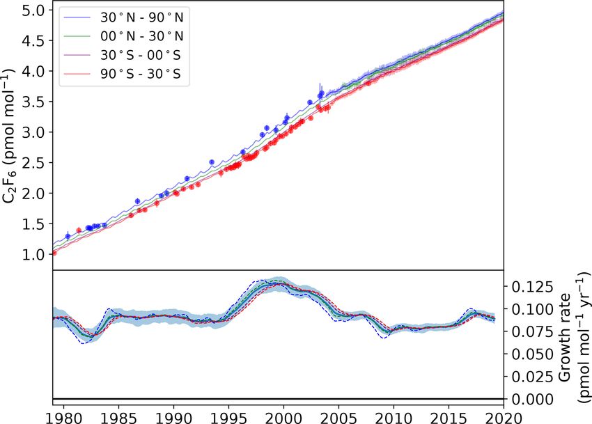
D. Say et al.: European emissions of CF4 , C2 F6 and C3 F8                                                                       2153

                                                                       nal by longitudinal resolution is 0.234◦ by 0.352◦ . We regard
                                                                       measurements as being sensitive to emissions from the sur-
                                                                       face when simulated particles in the model fall below 40 m
                                                                       above ground level (a.g.l.) within a 30 d period prior to the
                                                                       measurement. NAME simulates the release of 20 000 par-
                                                                       ticles per hourly measurement interval within the computa-
                                                                       tional domain −98 to 40◦ E and 11 to 79◦ N. At MHD and
                                                                       TAC, these particles were released from a 20 m vertical line
                                                                       centred on the sample inlet. At JFJ and CMN, the mountain
                                                                       meteorology presents additional challenges for the model. At
                                                                       these stations, we assumed a release point of 1000 m a.g.l. for
                                                                       JFJ and 500 m a.g.l. for CMN, representing a compromise be-
                                                                       tween the model surface altitude and the actual station height.
                                                                       The NAME model was run offline prior to the inversion and
                                                                       tailored to create a sensitivity matrix for a specific gas fol-
                                                                       lowing Arnold et al. (2018).
Figure 4. Modelled semi-hemispheric monthly average C3 F8 mole            InTEM estimates the spatial emissions of CF4 , C2 F6 and
fractions (30–90◦ N: blue; 0–30◦ N: green; 30–0◦ S: purple; 90–        C3 F8 by combining measurements, the sensitivities gener-
30◦ S: red). Monthly averaged baseline observations are shown as
                                                                       ated using NAME, any prior knowledge available about the
data points with 1σ error bars. The more sparse filled circles rep-
                                                                       emissions sources and magnitudes, and the uncertainty in
resent northern (blue) and southern (red) hemispheric air archive
samples. The solid trend lines were calculated using the AGAGE         these quantities. InTEM is a Bayesian inversion system that
12-box model with emissions from the inversion as input. The lower     uses a non-negative least-squares solver. This is described in
plot shows the model-derived mole fraction growth rate, smoothed       detail in Arnold et al. (2018). The baseline, or background,
with an approximate 1-year filter, for each semi-hemisphere (dashed    mole fraction is solved for within the inversion system. Prior
lines) and the global mean with 1σ uncertainty (solid line and shad-   baselines were estimated for MHD, JFJ and CMN using the
ing).                                                                  measurements at those sites. The prior baseline for TAC was
                                                                       assumed to be equivalent to the prior MHD baseline, since
                                                                       they occupy similar latitudes.
through the inversion, along with the uncertainty due to the              The measurement uncertainty was estimated to be a com-
prior constraint, to calculate the posterior emissions uncer-          bination of the precision described in Sect. 2.1 and the vari-
tainty.                                                                ability of three consecutive measurements centred around the
                                                                       measurement point. The observations were averaged into 4 h
2.4   Estimating European emissions using a regional                   windows. The model uncertainty was a combination of the
      inverse modelling technique                                      prior baseline uncertainty and the magnitude of the median
                                                                       pollution event at the measurement location per year. Obser-
We infer regional PFC emissions by combining atmospheric               vations recorded at TAC were selected when the difference
measurements (Sect. 2.1) and air histories, derived using the          between CH4 observations (made using a Picarro G2301)
atmospheric-dispersion model NAME (Jones et al., 2007),                at different heights on the mast during the 4 h period were
within the Met Office’s Inversion Technique for Emissions              less than 20 ppb; i.e. the air was well mixed in the verti-
Modelling (InTEM) framework. Numerous examples exist                   cal. Analysis of the meteorology during these selected times
within the literature that describe the use of InTEM for the           provided thresholds that were applied at MHD which only
estimation of long-lived greenhouse gas emissions (e.g. Man-           has one measurement height. Off-diagonal elements of the
ning et al., 2011; Say et al., 2016; Arnold et al., 2018; Rigby        model–observation uncertainty matrix were calculated by as-
et al., 2019; Mühle et al., 2019). In short, the simulated trans-      suming a temporal correlation timescale of 12 h. The sensi-
port of gas in the NAME atmospheric transport model cre-               tivity of the results to this arbitrary value is low for reason-
ates a sensitivity matrix that maps the spatial surface emis-          able changes – tests with 8 and 16 h windows showed that
sions to a modelled measurement. Meteorology from the UK               there was little discernible impact on the annually estimated
Met Office Unified Model (UM) (Walters et al., 2019), in-              national emissions.
cluding the nested high-resolution UK model (UKV) from                    For each inversion, the system used an a priori estimate
2014 onwards, drives the transport through advection, dif-             of emissions which were distributed uniformly over land, on
fusion and turbulence in NAME. The global UM and UKV                   which a prior distribution with very large uncertainty was
are available at 3- and 1-hourly resolutions, respectively. The        placed, ensuring that the posterior solution was informed
horizontal resolution of the global UM has increased from              entirely by the atmospheric measurements. Only two con-
∼ 40 km in 2003 to ∼ 12 km in 2020; the UKV is at ∼ 1.5 km             straints were applied a priori: (1) all grid cells were forced
over the UK and Ireland. The NAME output spatial latitudi-             to have a non-negative emission; (2) the nine grid cells cen-

https://doi.org/10.5194/acp-21-2149-2021                                                Atmos. Chem. Phys., 21, 2149–2164, 2021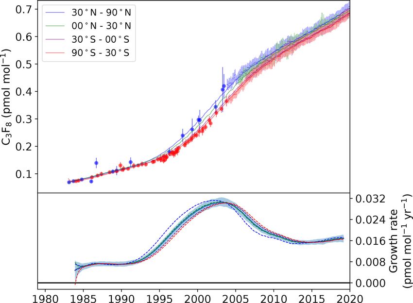
2154                                                              D. Say et al.: European emissions of CF4 , C2 F6 and C3 F8

tred on the locations of known PFC emitters, as reported to       Table 2. Global annual PFC emissions, estimated using the AGAGE
the E-PRTR, were specifically solved for. The E-PRTR only         12-box model – an extension of the work by Rigby et al. (2014),
reports total PFC emissions (e.g. the sum total of all individ-   Trudinger et al. (2016) and Engel and Rigby (2019) – in gigagrams
ual PFCs). Therefore, we define all E-PRTR locations for all      per year (Gg yr−1 ). Lower and upper uncertainty bounds corre-
three PFCs. Elsewhere in the domain, the spatial resolution of    spond to the 16th and 84th percentiles of the posterior model distri-
                                                                  bution, respectively.
the underlying grid was allowed to vary within each country,
with finer resolution in areas found to have high emissions
                                                                                   CF4               C2 F6              C3 F8
and high sensitivity to the measurements.
                                                                     2005    10.9 (10.0–12.0)     2.3 (2.2–2.5)   0.93 (0.87–0.98)
                                                                     2006    11.1 (10.5–12.2)     2.3 (2.2–2.4)   0.85 (0.80–0.89)
3     Results                                                        2007    10.9 (10.1–11.6)     2.3 (2.2–2.4)   0.76 (0.72–0.80)
                                                                     2008     10.3 (9.5–11.2)     2.1 (1.9–2.2)   0.69 (0.65–0.73)
                                                                     2009      9.7 (8.9–10.5)     1.9 (1.7–2.0)   0.64 (0.59–0.68)
3.1    Atmospheric trends and global emissions
                                                                     2010     10.2 (9.4–11.0)     1.9 (1.8–2.1)   0.61 (0.56–0.65)
                                                                     2011     10.9 (9.8–11.5)     1.9 (1.8–2.1)   0.57 (0.53–0.60)
The modelled and measured baseline atmospheric trends                2012    11.2 (10.3–11.9)     1.9 (1.8–2.0)   0.53 (0.49–0.58)
(1979–2019) of CF4 , C2 F6 and C3 F8 are shown in Figs. 2–           2013    11.2 (10.3–12.1)     1.9 (1.8–2.1)   0.52 (0.48–0.56)
4. Prior to the calculation of monthly baseline estimates, the       2014    11.3 (10.4–12.1)     2.0 (1.8–2.1)   0.51 (0.48–0.55)
AGAGE pollution algorithm (Cunnold et al., 2002) was used            2015    12.1 (11.1–13.0)     2.0 (1.8–2.1)   0.52 (0.48–0.55)
to remove regional pollution effects observed at each station.       2016    13.0 (12.2–14.0)     2.1 (2.0–2.3)   0.52 (0.49–0.55)
   For CF4 , a large increase in baseline mole fraction is evi-      2017    13.9 (13.0–15.0)     2.3 (2.1–2.4)   0.54 (0.50–0.57)
dent across all semi-hemispheres. The global mean increased          2018    14.1 (13.2–15.1)     2.2 (2.1–2.4)   0.55 (0.50–0.59)
from 52.1 ppt in 1979 to 85.5 ppt in 2019, representing an ap-       2019    13.9 (12.8–15.4)     2.2 (2.0–2.4)   0.56 (0.51–0.60)
proximate 3-fold increase following subtraction of the natu-
ral background. We observed significant variations in growth
rate across the measurement window. In 1979, the growth           C2 F6 as an etchant gas, is not known. The 2009 minimum
rate was estimated to be 1.3 ppt yr−1 but declined steadily to    was followed by a period of stagnation, with a near constant
a minimum of 0.6 ppt yr−1 by 2009. The drop in growth rate        growth rate between 2009 and 2013. Annual global emis-
observed around 2009 is probably due to a fall in aluminium       sions did not vary significantly during this period, remain-
production following the 2008 financial crisis. Production of     ing stable at ∼ 1.9 Gg yr−1 . However, there is some evidence
primary aluminium dropped by roughly 6 % (∼ 200 000 met-          for a resurgence in C2 F6 emissions post-2013. The global
ric tonnes) between 2008 and 2009 (IAI, 2020). Global emis-       growth rate in 2017 was estimated to be 0.09 ppt yr−1 , with
sions declined by 0.6 Gg over the same period (Table 2).          corresponding global emissions of 2.3 Gg yr−1 , the largest
However, more recent years have seen a renewed increase           observed since prior to the financial crisis.
in the growth rate of CF4 , rising from 0.7 ppt yr−1 in 2010         The global C3 F8 baseline mole fraction grew from an es-
to 0.9 ppt yr−1 in 2019. At 14.1 Gg yr−1 , emissions in 2018      timated 0.07 ppt in 1983 to 0.68 ppt in 2019. The large al-
are the largest observed since high-frequency measurements        most 10-fold increase shows that, in terms of relative growth,
began in 2003. Our work is consistent with Trudinger et al.       emissions of C3 F8 have increased sharply when compared to
(2016) and Engel and Rigby (2019), who showed the first in-       CF4 and C2 F6 . Unlike CF4 and C2 F6 , the aluminium indus-
crease in global CF4 emissions since the 1980s. Despite this,     try is not a major contributor of global emissions of C3 F8 ,
given global primary aluminium production has increased           though detectable concentrations have been observed in the
∼ 5-fold over the last 40 years (IAI, 2020), our estimates        outflow from smelter stacks (Fraser et al., 2003). Follow-
highlight the success of efficiency improvements and abate-       ing a period of relative stability between 1985 and 1992,
ment technology in reducing emissions of CF4 per tonne of         the growth rate increased rapidly, reaching a maximum of
aluminium produced.                                               0.03 ppt yr−1 in 2003. Thereafter, a period of steady decline
   The global C2 F6 baseline mole fraction grew from 1.1 ppt      saw the growth rate fall to 0.015 ppt yr−1 in 2014, with cor-
in 1979 to 4.8 ppt in 2019, an increase of more than 4-fold.      responding global emissions of 0.51 (0.48–0.55) Gg yr−1 . Of
The relative increase is larger than that of CF4 , suggesting     the three PFCs discussed, C3 F8 is the only gas for which a
that there are major sources of C2 F6 not linked to the alu-      pronounced “dip” in growth rate was not observed around
minium industry. The growth rate peaked in 1999 at an es-         the time of the financial crisis, perhaps indicative of the re-
timated 0.13 ppt yr−1 , followed by a sustained period of de-     silience of the semi-conductor industry to the crisis relative
cline to a minimum of 0.07 ppt yr−1 in 2009. As with CF4 ,        to aluminium producers. Since 2015, the global growth rate
the minimum rate of growth in 2009 is probably a result,          has remained comparatively stable, with no statistically sig-
at least in part, of the reduced demand for aluminium fol-        nificant trend in global emissions. Emissions in 2019 were
lowing the 2008 financial crisis. The effect of the crisis on     estimated to be 0.56 (0.51–0.60) Gg yr−1 .
demand for electronics, and therefore the consumption of

Atmos. Chem. Phys., 21, 2149–2164, 2021                                              https://doi.org/10.5194/acp-21-2149-2021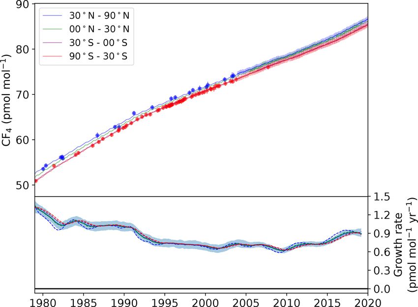
D. Say et al.: European emissions of CF4 , C2 F6 and C3 F8                                                                   2155

3.2     Northwest European PFC emissions                         site are the main driver of the recent observed increase in
                                                                 Ireland’s CF4 emissions.
We present estimates of PFC emissions in northwest Europe           The inferred spatial distribution of northwest European
(the United Kingdom; Ireland; France; Belgium, the Nether-       CF4 emissions is shown in Fig. 6. In 2005, regional emissions
lands and Luxembourg (collectively termed Benelux); and          were dominated by those from western Germany, roughly
Germany) using the procedure described in Sect. 2.4, based       consistent (accounting for transport errors) with the location
on the sensitivity of the measurements to emissions from         of three aluminium smelters in the Ruhr valley. Aluminium
these countries (see Fig. 1).                                    production is also the probable source of smaller emissions
   From 2005 to 2007 (2005 to 2010 for CF4 ), we only report     from southwest Norway and northern Denmark, although we
emissions for the UK, Ireland and Benelux, due to the lack       do not report national estimates for these countries. Alu-
of atmospheric measurements from continental Europe and          minium production in the Ruhr valley in Germany remains
therefore sensitivity to southern France and eastern Germany     a significant source of CF4 in later years, though emissions
during this period. Reported estimates for France and Ger-       from other areas and industries become apparent. Starting in
many (and the northwest Europe total) begin in 2008 (C2 F6       2010, strong emissions were found for southeast France and
and C3 F8 ) and 2010 (CF4 ), corresponding with the availabil-   northwest Italy. Southeast France has previously been linked
ity of measurements from JFJ (Table 1).                          to emissions of other halogenated species (Maione et al.,
                                                                 2014). Our results show that emissions from this region di-
3.2.1    CF4                                                     minished after 2015. In contrast, emissions from northwest
                                                                 Italy continued to grow until the end of the record. The E-
Annual CF4 emissions for northwest Europe are shown in           PRTR lists two PFC emitters in the region. The largest of
Fig. 5 and Table S1. Due to the considerable uncertainties,      these sources, a chemicals manufacturer located near the Ital-
we find no statistically significant trend in emissions from     ian city of Alessandria, is consistent with our emissions maps
the region over the measurement period (based on the 95 %        after 2010. This manufacturer reported total PFC emissions
uncertainty in the trend).                                       of 185 Mg in 2012, making it one of the largest emitters in
   European aluminium production dropped significantly           Europe. Interestingly, this region has previously been linked
during the measurement period, declining from 3.2 MT in          to considerable emissions of the hydrofluorocarbon, trifluo-
2004, to just 2.2 MT in 2016 (IAI, 2020). In that time, the      romethane (CHF3 , HFC-23) (Keller et al., 2011), though we
number of active European aluminium smelters also de-            are unable to ascertain whether theses gases share a common
clined, falling from 25 to 16. On average, northwest Europe      source.
accounted for 2.1 % of global emissions in 2010 (0.21 Gg            In comparison to other large European countries, emis-
in northwest Europe; 10.2 Gg globally) but only 0.7 % in         sions from the UK and Ireland are small throughout the
2018 (0.1 Gg in northwest Europe; 14.1 Gg globally). De-         reporting window. Between 2005 and 2012, emissions
spite no significant trend in northwest European emissions,      from northern England are consistent with the location of
global emissions increased considerably over the same pe-        the Lynemouth aluminium smelter, which was closed in
riod (Table 2), indicating that emissions from other regions     March 2012. After this date, the predominant UK source is
have increased. China was the largest producer of primary        located near the city of Manchester, consistent with the loca-
aluminium in 2019 (IAI, 2020). Comparison of our northwest       tion of an electronics manufacturer.
European estimates with compiled emissions reported to the          Emissions from the Benelux region are small and the un-
UNFCCC indicates a discrepancy between reporting meth-           certainties are large. In later years, the majority of these emis-
ods (Fig. 5) throughout most of the reporting window. Our        sions are consistent with the location of chemical manufac-
estimates are typically larger than the inventory, but some      turers. These emissions are in a similar location to a strong
agreement is observed from 2016 onwards.                         source of c-C4 F8 reported by Mühle et al. (2019), which the
   Of the individual countries/regions examined, Ireland is      authors attributed to the consumption of c-C4 F8 as an inter-
the only country whose reported emissions to the UNFCCC          mediate feed stock in the manufacture of polytetrafluoroethy-
have increased in recent years. The InTEM estimates mir-         lene (PTFE). There is no available evidence supporting the
ror this trend, though the uncertainties are considerable. Our   use of CF4 in PTFE manufacture, though the production of
estimates increased from 2.2 (0.0–5.7) Mg yr−1 in 2012 to        CF4 , perhaps as a byproduct, cannot be ruled out.
10.6 (4.3–16.9) Mg yr−1 in 2019. Ireland is not a producer
of aluminium metal, though it does have a bauxite refinery.      3.2.2   C2 F6
Therefore, its emissions of CF4 are probably due to con-
sumption by semi-conductor manufacturers. Across all years       Annual C2 F6 emissions are shown in Fig. 7 and Table S2.
of the E-PRTR (2007–2017), Ireland only reported emissions       Like CF4 , the uncertainty of our estimates for Germany and
from a single facility, a semi-conductor factory to the west     France, particularly in early years, is large and overall, there
of Dublin. From 2017 onwards, this source is evident in our      is no statistically significant trend in emissions from north-
spatial maps. It is therefore likely that emissions from this    west Europe over the measurement period (based on the 95 %

https://doi.org/10.5194/acp-21-2149-2021                                          Atmos. Chem. Phys., 21, 2149–2164, 2021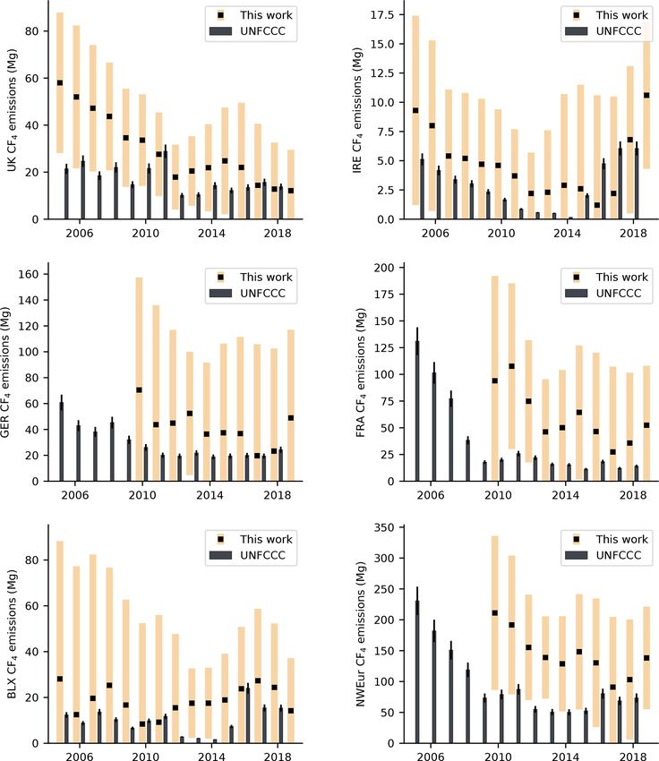
2156                                                                 D. Say et al.: European emissions of CF4 , C2 F6 and C3 F8

Figure 5. Annual CF4 emissions (2005–2019) for northwest European countries in Mg yr−1 . InTEM estimates are shown as black squares
with pale orange uncertainty bounds. Emissions reported to the UNFCCC (sum of individual reporting countries) are shown as black bars,
with an assumed uncertainty (black error bars) of 10 %. Note that UNFCCC data are only available up until 2018 inclusive.

uncertainty in the trend). When compared to global emis-             than the inventory, suggesting an under-reporting of emis-
sions, the average contribution of northwest Europe declined         sions during this period.
from 2.4 % in 2008 (0.05 Gg in northwest Europe; 2.1 Gg                 C2 F6 emissions maps are shown in Fig. 8. Unlike CF4 ,
globally) to 1.6 % in 2018 (0.03 Gg in northwest Europe;             whose emissions appear to be dominated by the aluminium
2.2 Gg globally).                                                    industry, the C2 F6 distribution is consistent with a greater
   Our work is in reasonable agreement with C2 F6 emissions          contribution from the electronics industry (Kim et al., 2014).
reported to the UNFCCC, particularly for Ireland between             For instance, in 2005, the two largest sources (on the out-
2006 and 2011, where our top-down estimates captured the             skirts of Dublin, Ireland, and Paris, France) correspond with
significant fall in emissions reported in Ireland’s national in-     the locations of electronics manufacturers, suggesting these
ventory. Elsewhere, our uncertainties typically overlap the          emissions are linked with the consumption of C2 F6 as an
average UNFCCC estimates, with the exception of Benelux,             etching gas. In contrast, emissions from the Ruhr valley in
where our emissions for 2013–2016 are significantly larger           Germany are small. By 2012, a source in northern Belgium,
                                                                     which is concurrent with the location of a basic chemicals

Atmos. Chem. Phys., 21, 2149–2164, 2021                                                https://doi.org/10.5194/acp-21-2149-2021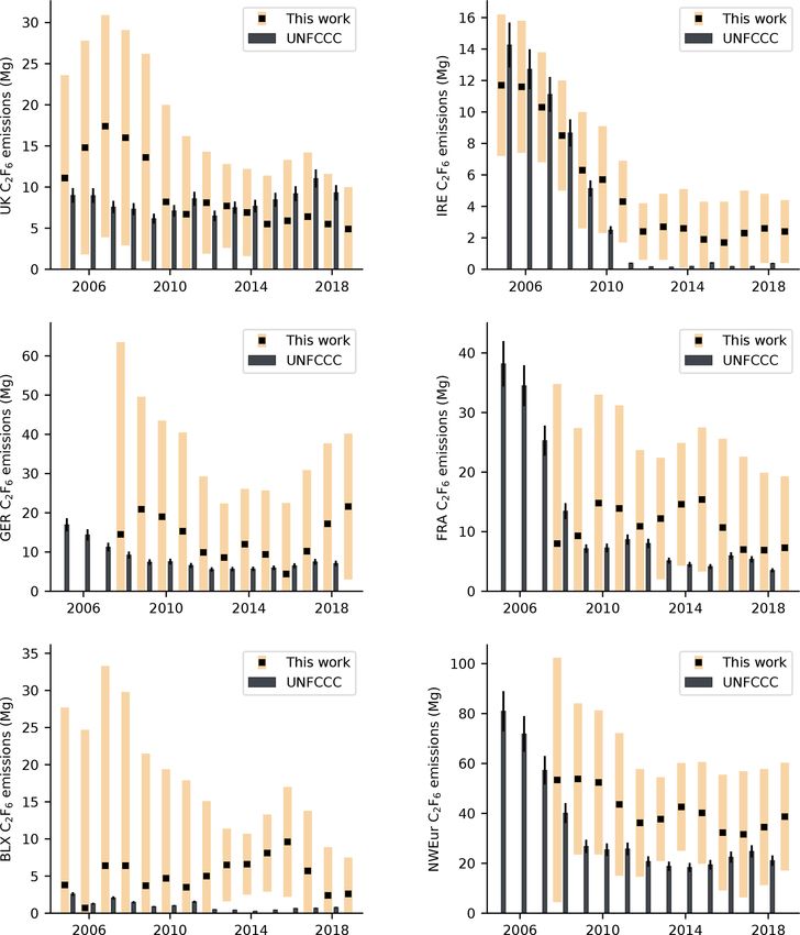
D. Say et al.: European emissions of CF4 , C2 F6 and C3 F8                                                                          2157

Figure 6. Northwest European CF4 emissions in kg km−2 yr−1 . (a) The a priori emissions field. With the exception of the oceans, emissions
were distributed uniformly across the model domain. A posteriori emissions are shown for (b) 2005, (c) 2012 and (d) 2019. Facilities
that reported PFC emissions to the E-PRTR in the selected year are shown as orange circles (aluminium smelters), triangles (electronics
manufacturers) and squares (chemical manufacturers, including petroleum products). Since the reporting period for the E-PRTR is shorter
than that of our measurements, 2005 and 2019 emissions are compared to the earliest (2007) and latest (2017) years of the E-PRTR database,
respectively. Note that the E-PRTR database reports cumulative PFC emissions.

manufacturer, dominates European emissions. The manufac-               ers are based here, these sources cannot be confirmed without
ture of basic chemicals also appear to be a source of C2 F6            further information from individual companies.
in southern France and northwest England. In contrast, the
emissions “hot-spot” located near Dublin in 2005 is greatly            3.2.3   C3 F8
diminished by 2012, in line with the planned phase-out of
C2 F6 in favour of NF3 by the manufacturer.                            Northwest European C3 F8 emissions are shown in Fig. 9 and
   By 2019, the spatial distribution of emissions is more var-         Table S3. As with CF4 and C2 F6 , northwest European emis-
ied. Large emissions are found for the Ruhr valley in Ger-             sions of C3 F8 exhibited no statistically significant trend over
many and likely originate from three aluminium smelters in             the measurements period. The contribution of northwest Eu-
the region that were also found to emit CF4 , which is known           rope to global emissions is considerably greater than other
to be co-emitted during the smelting process at a ratio of             PFCs −4.8 % in 2008 (0.03 Gg in northwest Europe; 0.69 Gg
around 0.1 kg kg−1 CF4 / C2 F6 (Kim et al., 2014). In Ireland,         globally) and 5.1 % by 2018 (0.03 Gg in northwest Europe;
emissions associated with electronics manufacture, located             0.55 Gg globally). Of the gases studied, C3 F8 is the only PFC
on the outskirts of Dublin, have ceased. However, signifi-             for which northwest Europe contributed a greater fraction of
cant emissions are now found further to the southwest. This            the global total in 2018 than it did in 2008. Several coun-
source region does not appear to be listed under the E-PRTR            tries, including France and Ireland, reported no emissions of
and may be a contributing factor in the small discrepancy              C3 F8 to the UNFCCC across the measurement window. In
between our work and the UNFCCC, from 2011 onwards.                    general, our work is in agreement with these reports, with
These emissions are situated in a comparable location to the           the uncertainty bounds of our estimates typically encapsu-
Irish city of Limerick. While several electronics manufactur-          lating 0 Mg yr−1 . Our work shows the UK to be the largest

https://doi.org/10.5194/acp-21-2149-2021                                                 Atmos. Chem. Phys., 21, 2149–2164, 2021
2158                                                                 D. Say et al.: European emissions of CF4 , C2 F6 and C3 F8

Figure 7. Annual C2 F6 emissions (2005–2019) for northwest European countries in Mg yr−1 . InTEM estimates are shown as black squares
with pale orange uncertainty bounds. Emissions reported to the UNFCCC (sum of individual reporting countries) are shown as black bars,
with an assumed uncertainty (black error bars) of 10 %. Note that UNFCCC data are only available up until 2018 inclusive.

emitter of C3 F8 in northwest Europe. In the early years of          are consistent with that found for C2 F6 and c-C4 F8 (Mühle
the record, and again after 2016, there is a significant dis-        et al., 2019), probably due to close vicinity of chemical in-
crepancy between reporting methods, potentially indicative           dustries or perhaps due to a common PFC source.
of under-reporting by UK emitters.                                      UK emissions of C3 F8 appear to be dominated by a sin-
   The spatial maps reveal few notable sources of C3 F8              gle source located in northwest England (Fig. 10). Facility
across continental Europe. The apparent reduction of con-            listings from the E-PRTR show a PFC manufacturer whose
tinental sources in later years may be due to the substitution       location is consistent with this source (Fig. 10). This com-
of C3 F8 in the semi-conductor industry by lower GWP alter-          pany is the only known manufacturer of C3 F8 in the UK and
natives. However, it is also likely that in the absence of Eu-       possibly in all of Europe.
ropean measurements prior to 2008 (when JFJ came online),
the inversion has less skill in inferring point source emis-
sions at such a distance from the receptor (MHD). In 2012,
the spatial maximum in emissions from the Benelux region

Atmos. Chem. Phys., 21, 2149–2164, 2021                                                https://doi.org/10.5194/acp-21-2149-2021
D. Say et al.: European emissions of CF4 , C2 F6 and C3 F8                                                                            2159

Figure 8. Northwest European C2 F6 emissions in kg km−2 yr−1 . (a) The a priori emissions field. With the exception of the oceans, emissions
were distributed uniformly across the model domain. A posteriori emissions are shown for (b) 2005, (c) 2012 and (d) 2019. Facilities
that reported PFC emissions to the E-PRTR in the selected year are shown as orange circles (aluminium smelters), triangles (electronics
manufacturers) and squares (chemical manufacturers, including petroleum products). Since the reporting period for the E-PRTR is shorter
than that of our measurements, 2005 and 2019 emissions are compared to the earliest (2007) and latest (2017) years of the E-PRTR database,
respectively. Note that the E-PRTR database reports cumulative PFC emissions.

3.2.4   UK C3 F8 emissions as a tracer for atmospheric                  fraction. This indicates that the assumed emissions rate is too
        transport                                                       small, or there are errors in the transport model (NAME). Al-
                                                                        ternatively, the current assumption, that emissions from the
If the facility in northwest England is the only source of C3 F8        site are released at a constant rate throughout the year, may
in northwest Europe, this gas could potentially be used as              also be an oversimplification – emissions are likely to vary
a tracer species for the validation of atmospheric transport            depending on the rate of production.
models, assuming that emissions are well defined. To test the              While atmospheric dispersion models, such as NAME,
validity of UK C3 F8 emissions as a potential tracer, the mole          are used extensively to simulate atmospheric transport, they
fraction at MHD was modelled by multiplying the NAME                    rely on simulated atmospheric dynamics that are subject to
sensitivity matrices (see Sect. 2.4) with an emissions grid,            considerable uncertainties. If emissions from this source in
where the UK’s total reported emissions of C3 F8 in 2014                northwest England were known better (e.g. by collaboration
(UNFCCC, 8.69 Mg yr−1 ) were placed in the grid cell corre-             with the company), then differences between the forward
sponding with the location of the PFC manufacturer. The re-             model and observed mole fractions might be used to improve
sulting time series was then compared to the MHD observa-               model transport or make estimates of transport uncertainties.
tions. Figure 11 shows the comparison of the forward model              Due to the long atmospheric lifetime of C3 F8 , photochemi-
with MHD C3 F8 observations for July–August 2014 (time                  cal loss processes do not need to be taken into account, thus
frame chosen for illustrative purposes). In general, pollu-             further reducing uncertainty. Quantifying these differences
tion events observed at MHD coincide with modelled events,              would be a useful means by which to assess and perhaps im-
though in the example shown, the magnitude of the mod-                  prove the performance of individual model simulations in fu-
elled events is significantly smaller than the observed mole            ture inverse modelling work.

https://doi.org/10.5194/acp-21-2149-2021                                                   Atmos. Chem. Phys., 21, 2149–2164, 2021
2160 D. Say et al.: European emissions of CF4 , C2 F6 and C3 F8
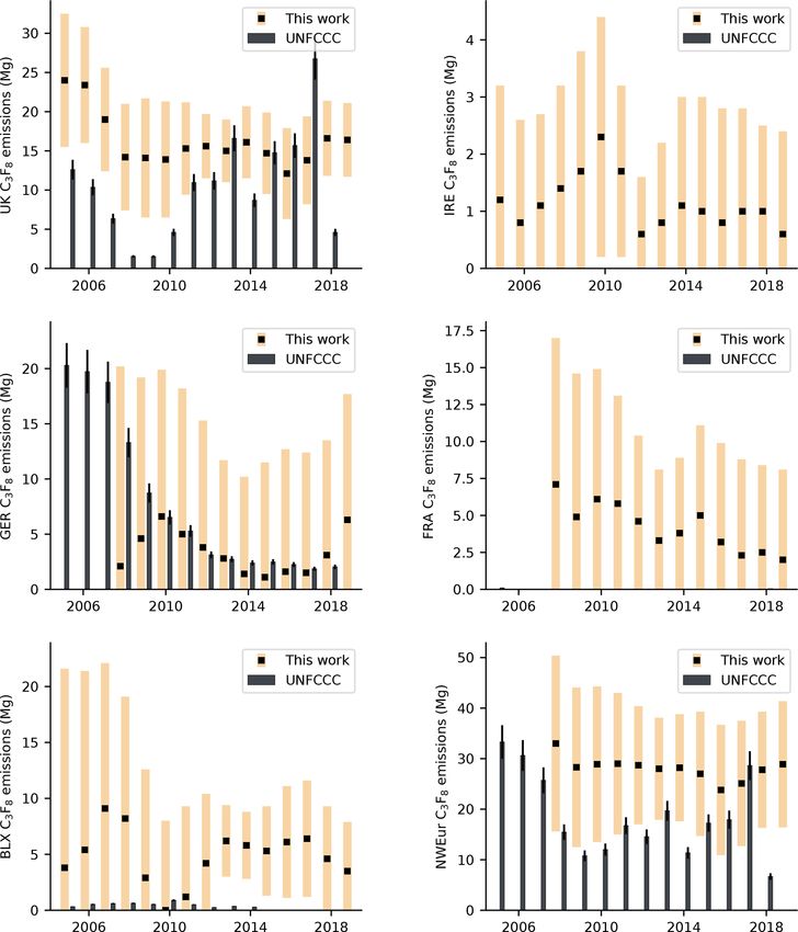
Figure 9. Annual C3 F8 emissions (2005–2019) for northwest European countries in Mg yr−1 . InTEM estimates are shown as black squares
with pale orange uncertainty bounds. Emissions reported to the UNFCCC (sum of individual reporting countries) are shown as black bars,
with an assumed uncertainty (black error bars) of 10 %. Note that UNFCCC data are only available up until 2018 inclusive.
4 Conclusions C2 F6 , a maximum growth rate of 0.125 ppt yr−1 was ob-
served around 1999, followed by a period of steady decline.
We have presented measurements of tetrafluoromethane Like with CF4 , we found a renewed increase in the global
(CF4 , PFC-14), hexafluoroethane (C2 F6 , PFC-116) and growth rate after 2011. C3 F8 exhibited a rapid increase in
octafluoropropane (C3 F8 , PFC-218) from the AGAGE net- growth rate, starting in the early 1990s and ending in the
work. We combined measurements from five background sta- early 2000s, followed by steady decline until 2013. In recent
tions, in conjunction with a box model, to infer global trends. years, a small increase in growth rate was observed.
For CF4 , the global mean baseline mole fraction increased We used observations from four European observatories to
by ∼ 33 ppt between 1979 and 2019. The global growth rate infer PFC emissions from northwest Europe. Between 2010
declined across much of the measurement period, falling to and 2019, northwest European emissions of CF4 exhibited
a minimum of 0.6 ppt yr−1 around the time of the 2008 fi- no statistically significant trend, despite an increase in global
nancial crisis. However, the growth rate began to rise again aluminium production and continued demand for electronic
after 2011, consistent with increasing global emissions. For components, consistent with growth in emissions from other
Atmos. Chem. Phys., 21, 2149–2164, 2021 https://doi.org/10.5194/acp-21-2149-2021D. Say et al.: European emissions of CF4 , C2 F6 and C3 F8 2161
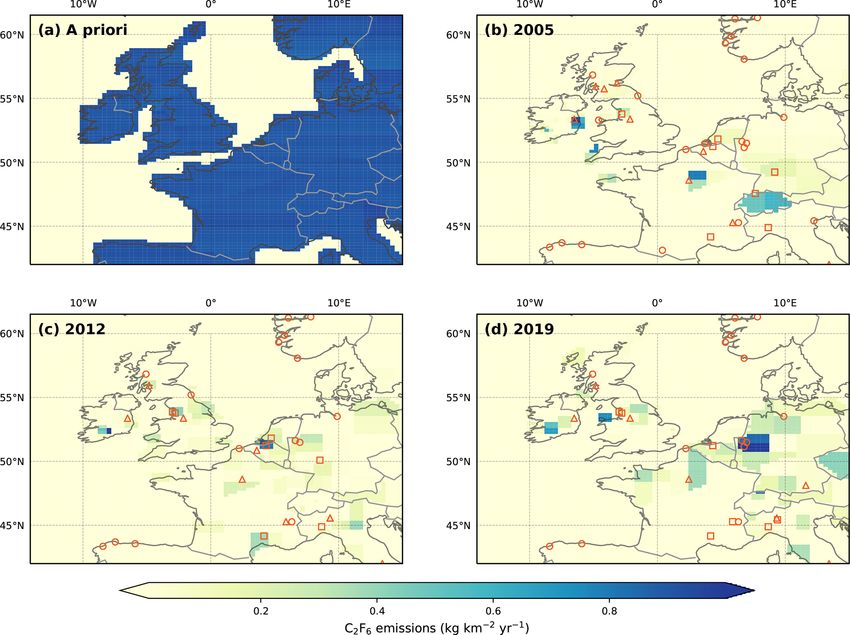
Figure 10. Northwest European C3 F8 emissions in kg km−2 yr−1 . (a) The a priori emissions field. With the exception of the oceans,
emissions were distributed uniformly across the model domain. A posteriori emissions are shown for (b) 2005, (c) 2012 and (d) 2019.
Facilities that reported PFC emissions to the E-PRTR in the selected year are shown as orange circles (aluminium smelters), triangles
(electronics manufacturers) and squares (chemical manufacturers, including petroleum products). Since the reporting period for the E-PRTR
is shorter than that of our measurements, 2005 and 2019 emissions are compared to the earliest (2007) and latest (2017) years of the E-PRTR
database, respectively. Note that the E-PRTR database reports cumulative PFC emissions.
regions. In early years, emissions were predominantly con-
sistent with the locations of aluminium smelters. However,
in more recent years, the largest source of CF4 was north-
west Italy. These emissions might be linked to a chemicals
manufacturer that reports substantial PFC emissions to the
E-PRTR.
Likewise for C2 F6 , no significant trend was observed for
northwest European emissions from 2008 until 2019. A no-
table fall in emissions from Ireland was observed between
2007 and 2012. This trend was mirrored by Ireland’s na-
tional inventory report and appears to be linked with an elec-
tronics manufacture on the outskirts Dublin. By 2019, the
largest source of C2 F6 in northwest Europe was western Ger-
many, most notably the Ruhr valley region in which three
aluminium smelters are found. Northwest European C3 F8
Figure 11. Comparison of measured (blue dots) and modelled (red emissions were stable over the measurement period. Several
line) C3 F8 mole fractions at MHD for July–August 2014. Dates are countries, including France and Ireland, reported no emis-
chosen for illustrative purposes only. sions of C3 F8 , which our results are consistent with. With
the exception of a small source in Benelux, we found north-
https://doi.org/10.5194/acp-21-2149-2021 Atmos. Chem. Phys., 21, 2149–2164, 20212162 D. Say et al.: European emissions of CF4 , C2 F6 and C3 F8
west European emissions of C3 F8 were dominated by a sin- by the Australian Bureau of Meteorology, CSIRO and NASA con-
gle source in northwest England, consistent with the location tract NNX16AC98G to MIT with sub-award no. 5710004055 to
of a PFC manufacturer. We explored the potential of using CSIRO. Operations at the O. Vittori station (Monte Cimone) are
this facility in a tracer release experiment and showed that, if supported by the National Research Council of Italy. Trinidad
accurate high-frequency emissions data were made available, Head, Cape Matatula and data processing and calibration across the
AGAGE network were funded by NASA grant nos. NNX16AC96G
this site could be used to provide useful information related
and NNX16AC97G to the Scripps Institution of Oceanography.
to transport model performance. Luke M. Western and Matthew Rigby were funded by NERC
grant nos. NE/N016548/1 and NE/S004211/1, and Matthew Rigby
was funded under NERC grant no. NE/M014851/1. Inverse anal-
Code and data availability. Atmospheric measurement data from ysis was carried out on hardware supported by NERC grant
AGAGE stations are available from the AGAGE website (http: no. NE/L013088/1.
//agage.mit.edu/data/agage-data, Prinn et al., 2020). Data from the
Tacolneston observatory are available from the Centre for Envi-
ronmental Data Analysis (CEDA) data archive (https://catalogue.
Review statement. This paper was edited by Andreas Hofzumahaus
ceda.ac.uk/uuid/a18f43456c364789aac726ed365e41d1, O’Doherty
and reviewed by two anonymous referees.
et al., 2019). AGAGE 12-box model code will be made available
upon request by contacting Matt Rigby. Licenses to use NAME and
InTEM are available for research purposes via a request to the UK
Met Office or on request from Alistair Manning. References
Arnold, T., Manning, A. J., Kim, J., Li, S., Webster, H., Thom-
Supplement. The supplement related to this article is available on- son, D., Mühle, J., Weiss, R. F., Park, S., and O’Doherty, S.: In-
line at: https://doi.org/10.5194/acp-21-2149-2021-supplement. verse modelling of CF4 and NF3 emissions in East Asia, Atmos.
Chem. Phys., 18, 13305–13320, https://doi.org/10.5194/acp-18-
13305-2018, 2018.
Author contributions. Measurement data were collected by SO’D, Burkholder, J. B., Hodnebrog, Ø., and Orkin, V. L.: Annex
DY, AW, DS, SR, MKV, MM, JA, PBK, JM, RFW and RGP. CMH 1: Summary of abundances, lifetimes, ozone depletion po-
produced and maintained the gravimetric SIO calibration scales tentials (ODPs), radiative efficiences (REs), global warming
for these gases. AJM conducted the NAME runs and ran the In- potentials (GWPs), and global temperature change potentials
TEM inverse model. MR performed the global 12-box model in- (GTPs), Vol. 58, Global Ozone Research and Monitoring Project,
versions. BE performed the C3 F8 forward model runs. DS and LW World Meteorological Organization, Geneva, Switzerland, avail-
analysed InTEM and forward model output. DS and LW wrote the able at: https://csl.noaa.gov/assessments/ozone/2018/downloads/
manuscript, with contributions from all co-authors. AppendixA_2018OzoneAssessment.pdf (last access: 6 Septem-
ber 2020), 2019.
Cai, B., Liu, H., Kou, F., Yang, Y., Yao, B., Chen, X., Wong, D.
Competing interests. The authors declare that they have no conflict S., Zhang, L., Li, J., Kuang, G., Chen, L., Zheng, J., Guan, D.,
of interest. and Shan, Y.: Estimating perfluorocarbon emission factors for
industrial rare earth metal electrolysis, Resour. Conserv. Recycl.,
136, 315–323, 2018.
Cicerone, R. J.: Atmospheric carbon tetrafluoride: A nearly inert
Acknowledgements. The authors would like to thank the on-site
gas, Science, 206, 59–61, 1979.
technicians across the AGAGE network for their cooperation and
Cunnold, D., Prinn, R., Rasmussen, R., Simmonds, P., Alyea, F.,
efforts in maintaining AGAGE instrumentation.
Cardelino, C., Crawford, A., Fraser, P., and Rosen, R.: The at-
mospheric lifetime experiment: 3. Lifetime methodology and ap-
plication to three years of CFCl3 data, J. Geophys. Res.-Oceans,
Financial support. The operations of Mace Head and Tacolneston 88, 8379–8400, 1983.
were funded by the UK Department of Business, Energy and Indus- Cunnold, D., Steele, L., Fraser, P., Simmonds, P., Prinn, R., Weiss,
trial Strategy (BEIS) through contract no. 1537/06/2018 to the Uni- R., Porter, L., O’Doherty, S., Langenfelds, R., Krummel, P.,
versity of Bristol. The operations of Mace Head and Ragged Point Wang, H., Emmons, L., Tie, X., and Dlugokencky, E.: In situ
were also partly funded under NASA contract no. NNX16AC98G measurements of atmospheric methane at GAGE/AGAGE sites
to MIT with a sub-award (no. 5710002970) to the University of during 1985-2000 and resulting source inferences, J. Geophys.
Bristol. Ragged Point was also partly funded by NOAA grant Res-Atmos., 107, 4225, https://doi.org/10.1029/2001JD001226,
no. RA133R15CN0008 to the University of Bristol. Support for 2002.
the observations at Jungfraujoch comes through Swiss national pro- EDGAR: Emission Database for Global Atmospheric Research
grammes HALCLIM and CLIMGAS-CH (Swiss Federal Office (EDGAR), release version 4.0, available at: https://edgar.jrc.ec.
for the Environment, FOEN), the International Foundation High europa.eu/ (last access: 6 September 2020), 2009.
Altitude Research Stations Jungfraujoch and Gornergrat (HFSJG) Engel, A. and Rigby, M.: Chapter 1: Update on Ozone Depleting
and ICOS-CH (Integrated Carbon Observation System Research Substances (ODSs) and Other Gases of Interest to the Mon-
Infrastructure). Observations at Cape Grim are supported largely treal Protocol, in: Scientific Assessment of Ozone Depletion:
Atmos. Chem. Phys., 21, 2149–2164, 2021 https://doi.org/10.5194/acp-21-2149-2021D. Say et al.: European emissions of CF4 , C2 F6 and C3 F8 2163 2018, Vol. 58 of Global Ozone Research and Monitoring Project, and octafluoropropane, Atmos. Chem. Phys., 10, 5145–5164, World Meteorological Organization, Geneva, Switzerland, avail- https://doi.org/10.5194/acp-10-5145-2010, 2010. able at: https://csl.noaa.gov/assessments/ozone/2018/downloads/ Mühle, J., Trudinger, C. M., Western, L. M., Rigby, M., Vollmer, Chapter1_2018OzoneAssessment.pdf (last access: 6 Septem- M. K., Park, S., Manning, A. J., Say, D., Ganesan, A., Steele, ber 2020), 2019. L. P., Ivy, D. J., Arnold, T., Li, S., Stohl, A., Harth, C. M., Fraser, P., Steele, P., and Cooksey, M.: PFC and carbon dioxide Salameh, P. K., McCulloch, A., O’Doherty, S., Park, M.-K., Jo, emissions from an Australian aluminium smelter using time- C. O., Young, D., Stanley, K. M., Krummel, P. B., Mitrevski, integrated stack sampling and GC-MS, GC-FID analysis, in: B., Hermansen, O., Lunder, C., Evangeliou, N., Yao, B., Kim, J., Light Metals 2013, Springer US, Boston, MA, 871–876, 2003. Hmiel, B., Buizert, C., Petrenko, V. V., Arduini, J., Maione, M., Harnisch, J. and Eisenhauer, A.: Natural CF4 and SF6 on Earth, Etheridge, D. M., Michalopoulou, E., Czerniak, M., Severing- Geophys. Res. Lett., 25, 2401–2404, 1998. haus, J. P., Reimann, S., Simmonds, P. G., Fraser, P. J., Prinn, R. IAI: Primary aluminium production statistics, available at: http: G., and Weiss, R. F.: Perfluorocyclobutane (PFC-318, c-C4 F8 ) in //www.world-aluminium.org/statistics/, last access: 6 Septem- the global atmosphere, Atmos. Chem. Phys., 19, 10335–10359, ber 2020. https://doi.org/10.5194/acp-19-10335-2019, 2019. Jones, A., Thomson, D., Hort, M., and Devenish, B.: The UK Met O’Doherty, S., Say, D., and Stanley, K.: Deriving Emissions Office’s next-generation atmospheric dispersion model, NAME related to Climate Change Network: CO2 , CH4 , N2 O, III, in: Air pollution modeling and its application XVII, Springer SF6, CO and halocarbon measurements from Tacolne- US, Boston, MA, 580–589, 2007. ston Tall Tower, Norfolk, Centre for Environmental Data Keller, C. A., Brunner, D., Henne, S., Vollmer, M. K., O’Doherty, Analysis, available at: https://catalogue.ceda.ac.uk/uuid/ S., and Reimann, S.: Evidence for under-reported western Euro- ae483e02e5c345c59c2b72ac46574103 (last access: 6 September pean emissions of the potent greenhouse gas HFC-23, Geophys. 2020), 2019. Res. Lett., 38, L15808, https://doi.org/10.1029/2011GL047976, Prinn, R. G., Weiss, R. F., Arduini, J., Arnold, T., DeWitt, H. L., 2011. Fraser, P. J., Ganesan, A. L., Gasore, J., Harth, C. M., Her- Kim, J., Fraser, P. J., Li, S., Mühle, J., Ganesan, A. L., Krummel, mansen, O., Kim, J., Krummel, P. B., Li, S., Loh, Z. M., Lun- P. B., Steele, L. P., Park, S., Kim, S-K., Park, M.-K., Arnold, T., der, C. R., Maione, M., Manning, A. J., Miller, B. R., Mitrevski, Harth, C. M., Salameh, P. K., Prinn, R. G., Weiss, R. F., and Kim, B., Mühle, J., O’Doherty, S., Park, S., Reimann, S., Rigby, M., K.-R.: Quantifying aluminum and semiconductor industry per- Saito, T., Salameh, P. K., Schmidt, R., Simmonds, P. G., Steele, fluorocarbon emissions from atmospheric measurements, Geo- L. P., Vollmer, M. K., Wang, R. H., Yao, B., Yokouchi, Y., Young, phys. Res. Lett., 41, 4787–4794, 2014. D., and Zhou, L.: History of chemically and radiatively impor- Maione, M., Giostra, U., Arduini, J., Furlani, F., Graziosi, F., Vullo, tant atmospheric gases from the Advanced Global Atmospheric E. L., and Bonasoni, P.: Ten years of continuous observations of Gases Experiment (AGAGE), Earth Syst. Sci. Data, 10, 985– stratospheric ozone depleting gases at Monte Cimone (Italy) – 1018, https://doi.org/10.5194/essd-10-985-2018, 2018. Comments on the effectiveness of the Montreal Protocol from a Prinn, R. G., Weiss, R. F., Arduini, J., Arnold, T., Fraser, P. J., regional perspective, Sci. Total Environ., 445, 155–164, 2013. Ganesan, A. L., Gasore, J., Harth, C. M., Hermansen, O., Kim, Maione, M., Graziosi, F., Arduini, J., Furlani, F., Giostra, U., J., Krummel, P. B., Li, S., Loh, Z. M., Lunder, C. R., Maione, Blake, D. R., Bonasoni, P., Fang, X., Montzka, S. A., O’Doherty, M., Manning, A. J., Miller, B. R., Mitrevski, B., Mühle, J., S. J., Reimann, S., Stohl, A., and Vollmer, M. K.: Esti- O’Doherty, S., Park, S., Reimann, S., Rigby, M., Salameh, P. mates of European emissions of methyl chloroform using a K., Schmidt, R., Simmonds, P. G., Steele, L. P., Vollmer, M. Bayesian inversion method, Atmos. Chem. Phys., 14, 9755– K., Wang, R. H., and Young, D.: The ALE/GAGE/AGAGE Data 9770, https://doi.org/10.5194/acp-14-9755-2014, 2014. Base http://agage.mit.edu/data, last access: 6 September 2020. Manning, A., O’Doherty, S., Jones, A., Simmonds, P., and Ravishankara, A., Solomon, S., Turnipseed, A. A., and Warren, R.: Derwent, R.: Estimating UK methane and nitrous oxide Atmospheric lifetimes of long-lived halogenated species, Sci- emissions from 1990 to 2007 using an inversion mod- ence, 259, 194–199, 1993. eling approach, J. Geophys. Res.-Atmos., 116, D02305, Rigby, M., Prinn, R., O’Doherty, S., Miller, B., Ivy, D., Mühle, J., https://doi.org/10.1029/2010JD014763, 2011. Harth, C., Salameh, P., Arnold, T., Weiss, R., et al.: Recent and Miller, B. R., Weiss, R. F., Salameh, P. K., Tanhua, T., Greally, B. R., future trends in synthetic greenhouse gas radiative forcing, Geo- Mühle, J., and Simmonds, P. G.: Medusa: A sample preconcen- phys. Res. Lett, 41, 2623–2630, 2014. tration and GC/MS detector system for in situ measurements of Rigby, M., Park, S., Saito, T., Western, L. M., Redington, A. L., atmospheric trace halocarbons, hydrocarbons, and sulfur com- Fang, X., Henne, S., Manning, A. J., Prinn, R. G., Dutton, G. pounds, Anal. Chem., 80, 1536–1545, 2008. S., Fraser, P. J., Ganesan, A. L., Hall, B. D., Harth, C. M., Kim, Morris, R. A., Miller, T. M., Viggiano, A., Paulson, J. F., Solomon, J., Kim, K.-R., Krummel, P. B., Lee, T., Li, S., Liang, Q., Lunt, S., and Reid, G.: Effects of electron and ion reactions on at- M. F., Montzka, S. A., Muhle, J., O’Doherty, S., Park, M.-K., mospheric lifetimes of fully fluorinated compounds, J. Geophys. Reimann, S., Salameh, P. K., Simmonds, P., Tunnicliffe, R. L., Res.-Atmos., 100, 1287–1294, 1995. Weiss, R. F., Yokouchi, Y., and Young, D.: Increase in CFC- Mühle, J., Ganesan, A. L., Miller, B. R., Salameh, P. K., Harth, 11 emissions from eastern China based on atmospheric obser- C. M., Greally, B. R., Rigby, M., Porter, L. W., Steele, L. P., vations, Nature, 569, 546–550, 2019. Trudinger, C. M., Krummel, P. B., O’Doherty, S., Fraser, P. J., Rigby, M., Prinn, R. G., O’Doherty, S., Montzka, S. A., McCulloch, Simmonds, P. G., Prinn, R. G., and Weiss, R. F.: Perfluorocarbons A., Harth, C. M., Mühle, J., Salameh, P. K., Weiss, R. F., Young, in the global atmosphere: tetrafluoromethane, hexafluoroethane, D., Simmonds, P. G., Hall, B. D., Dutton, G. S., Nance, D., Mon- https://doi.org/10.5194/acp-21-2149-2021 Atmos. Chem. Phys., 21, 2149–2164, 2021
You can also read