High-Frequency radar measurements with CODARs in the region of Nice: improved calibration and performances

Generated using the official AMS LTEX template v5.0 two-column layout. This work has been submitted for
 publication. Copyright in this work may be transferred without further notice, and this version may no
 longer be accessible.

 High-Frequency radar measurements with CODARs in the region of Nice:
 improved calibration and performances
 Charles-Antoine Guérin∗ , Dylan Dumas, Anne Molcard,
 Céline Quentin, Bruno Zakardjian, Anthony Gramoullé
 MIO, Université de Toulon, Aix-Marseille Univ, CNRS, IRD, Toulon, France
arXiv:2102.04507v1 [physics.ao-ph] 8 Feb 2021

 Maristella Berta
 ISMAR, CNR, La Spezia, Italy

 ABSTRACT

 We report on the installation and first results of one compact oceanographic radar in the region of Nice for a long-term
 observation of the coastal surface currents in the North-West Mediterranean Sea. We describe the specific processing and
 calibration techniques which were developed at the laboratory to produce high-quality radial surface current maps. In particular,
 we propose an original self-calibration technique of the antenna patterns, which is based on the sole analysis of the databasis
 and does not require any shipborne transponder or other external transmitters. The relevance of the self-calibration technique
 and the accuracy of inverted surface currents have been assessed with the launch of 40 drifters that remained under the radar
 coverage for about 10 days.

 1. Introduction dard performances proposed by the commercial tool-
 box suit can be greatly improved by using a specific
 In recent years there has been a growing European
 home-made processing, which can compensate for
 effort for the integrated observation of the Mediter-
 some defects of the installation. One of the main
 ranean Sea (e.g. Bellomo et al. (2015)). One of the
 limitations of such radar is related to its weak az-
 current challenges for the monitoring of the oceanic
 imuthal resolution, which is the counterpart of its
 circulation in the region is to develop and maintain
 compactness, and the touchy calibration of the com-
 a spatially and temporally dense network of High-
 plex antenna gains. As it is well known, the accu-
 Frequency Radars (HFR) for a continuous cover-
 rate characterization of the antenna patterns is a key
 age of the surface currents along the Mediterranean
 point in the Direction Finding (DF) technique which
 coasts Quentin et al. (2013). In the framework of
 is employed to obtain the azimuthal discrimination of
 the long-term French observation program “Mediter-
 radar echos with compact HFR systems. The antenna
 ranean Ocean Observing System for the Environ-
 system in real conditions undergoes in general some
 ment” (MOOSE (2008-); Coppola et al. (2019)) and
 distortion with respect to the factory settings and a
 more recently the EU Interreg Marittimo “Sicomar-
 precise on-site calibration of the individual antenna
 Plus” project (SICOMAR-PLUS (2018)), our labo-
 responses is required before proceeding to surface
 ratory has installed a pair of HFR of SeaSonde type
 current mapping.
 (CODAR Ocean Sensors, Ltd) in the region of Nice.
 In this report we describe the first operational HFR
 One of them has been operational since 2013 in Saint-
 site of Saint-Jean Cap Ferrat and its specificity (Sec-
 Jean Cap Ferrat, 2 km East of Nice. The other has
 tion 2) and we recall the principle of surface current
 been recently installed at the French-Italian border in
 mapping in this context. The key point is the appropri-
 the Port of Menton and is still under test.
 ate utilization of DF algorithm to resolve the surface
 CODARs are commonly used instruments in the
 current in azimuth, a process which goes through the
 oceanographic community; they have a dedicated
 software which in principle does not require any spe- application of the MUSIC algorithm (Section 3). We
 cific skills in the field of radar instrumentation and present some techniques from the user point of view
 signal processing. However, we found that the stan- which have a drastic impact on the quality of the re-
 sult. We describe a recent ship experiment to measure
 the real antenna pattern following the standard pro-
 ∗ Corresponding author: Charles-Antoine Guérin,
 cedure and we give a detailed review of the involved
 guerin@univ-tln.fr

 1

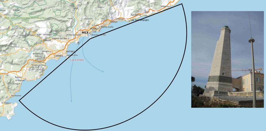
2 AMS JOURNAL NAME

radar signal processing steps (Section 4). In Section only 28 m from the 34 m high light house tower which
5, we propose a novel self-calibration technique based shields a small angular sector to the West. Electronic
on the mere analysis of the recorded Doppler spectra. devices including transmitter and receiver as well as
This method does not require any specific calibration the computer device (under MacOS system) control-
campaign and allows an easy update of the calibra- ling the equipment are hosted in an air-conditioned
tion as time goes by. We compare the radial surface enclosure as recommended (Mantovani et al. (2020)).
current maps obtained with 3 types of antenna pattern Albeit far from ideal, this configuration was found
(ideal, measured, self-calibrated) and assess them in the best compromise given the field constraints. The
the light of a recent oceanographic campaign pro- magnetic compass direction of the receive antenna
viding the in situ measurements of surface current by sighting arrow is about 160 degrees corresponding to
means of a set of 40 drifters (Section 6). We show that a theoretical bearing of 207 degree true North Clock
the best agreement is obtained with the self-calibrated Wise (NCW) after correction of the magnetic declina-
antenna patterns while the improvement brought by tion. The geometry of the coast between the Cape of
the measured pattern over the ideal is marginal. Antibes on the Western side and Cape Martin on the
 Eastern side allows viewing an angular sector from
2. Radar sites history and description 60◦ to 225◦ NCW but the distance between the Sea-
 Sonde and the sea remains constant (at about 50 m)
 The installation of one CODAR SeaSonde sensor
 only from 135◦ to 315◦ NCW. The vicinity of the
in the region of Nice was initially driven by the need
 lighthouse tower and the increased ground distance
to monitor the local oceanic circulation in the frame-
 are expected to limit the performances of the radar in
work of the MOOSE network Quentin et al. (2014).
 the other azimuthal directions.
The main objective was to properly track the Northern
Current (NC), which is the dominant stream flowing
along the continental slope. It transports warm and
salty Levantine Intermediate Water at intermediate
depths and thereby affects the properties of the West-
ern Mediterranean Deep Water formed downstream
off the Gulf of Lion. These radar sites are com-
plementary to another site located in the region of
Toulon downstream the NC (Dumas et al. (2020)).
The choice of this instrument was mainly motivated
by its compactness which is an absolute requirement
in the densely urbanized coastal zone of the French Fig. 1. Location and theoretical coverage of the SeaSonde
riviera. The HFR station was initially meant to cover CODAR installed in Saint-Jean Cap Ferrat. The field of view is
 limited to the West by the Cape of Antibes and to the East by
the geographical area surrounding a mooring site re- Cape Saint Ampelio. The arc of circle marks a typical 65 km
ferred to as “DYFAMED” for the long-term obser- coverage. The SeaSonde mast at the lighthouse of Saint-Jean Cap
vation of the core parameters of the water column Ferrat (upper right).
(Coppola et al. (2018, 2019)). The combination of
the time series describing the vertical structure and
the HFR currents is essential for the characterization 3. Radial current extraction with CODARs
of the full 3D structures of circulation observed in
the area (Berta et al. (2018); Coppola et al. (2018); As it relies on a compact antenna array, the CODAR
Manso-Narvarte et al. (2020)). This mooring site is uses DF algorithms to resolve the surface current in
located 50 km offshore and a medium range HFR (9- azimuth, which is the most critical step in the pro-
20 MHz operating frequency) is well adapted to cover cessing chain of the radar data and requires a reliable
the surface current measurements from the coast to knowledge of the complex antenna gains. We recall
70-80 km away. that the antenna system is composed of two cross-loop
 The SeaSonde HFR operates at a 13.5 MHz cen- antennas and one monopole, with ideal patterns:
tral frequency within a full bandwidth of 100 kHz
allowing for 1.5 km range resolution. It is sited at 1 ( ) = cos( − ),
the lighthouse of Saint-Jean Cap Ferrat where it is 2 ( ) = sin( − ), (3.1)
installed on a flat terrace less than 90 m away from 3 ( ) = 1
the sea at an altitude of about 30 meter (Figure 1). It
is equipped with co-located receive and transmit an- where is the main bearing. In its standard mode
tennas mounted on a 7 meter mast. It is separated by the CODAR SeaSonde uses Interrupted Frequency

3

Modulated Continuous Wave with chirps of duration where = 1 or 2 is the number of sources. In prac-
0.25 sec and equal intra-pulse duration, leading to a tice, the quality of the MUSIC estimation relies on the
2 Hz sampling rate for the range-resolved backscat- appropriate setting of a certain number of threshold
tered temporal signal on each antenna. A Fast parameters as well as some numerical recipes which
Fourier Transform is applied to these time series to we detail here.
form the co- and cross-Doppler spectra = b∗
 b 
 (i) Normalization of the covariance matrix The
(9 elements), where b denotes the Discrete Fourier covariance matrix, because it is obtained from a
Transform and ∗ the complex conjugate. A typical nonlinear combination of the antenna channels, is
integration time of 256 sec (512 chirps) is employed strongly dependent on the individual calibration of
to obtain the individual complex Doppler spectra the signals recorder on each antenna. In particular,
(512 Doppler bins, “CSQ” files), which are averaged rescaling one channel in amplitude, say antenna 1,
other 15 min (4 CSQ) to produce mean Doppler spec- will drastically affects the eigenvalues and eigenvec-
tra at an update rate of 10 min (“CSS” files). tors of the covariance matrix, hence the whole DF
A series of 7 such spectra are further combined to process. This cannot be compensated by a simple
produce an ensemble average over 75 min (with up- rescaling of the steering vector. It is therefore impor-
date rate of 60 min) and estimate a covariance matrix tant that the diagonal coefficients of the covariance
Σ = h i for each Doppler ray and each range bin. matrix have the same order of magnitude. This im-
The Direction of Arrival (DoA) corresponding to a plies that the Doppler co-spectra should also have the
given frequency shift (hence to a given radial surface same order of magnitude, aside from angular vari-
current) is determined from the MUSIC algorithm ations due to the antenna pattern. For this it is not
 enough to form the “loop amplitude ratios”, which are
(Schmidt (1986)). A Singular Value Decomposition
 the signals received on antenna loop 1 and 2 normal-
(SVD) of each covariance matrix is performed, with
 ized by the reference signal received on the monopole
eigenvalues 1 ≥ 2 ≥ 3 ≥ 0 and normalized eigen-
 antenna 3, because the gains of antenna 1 and 2 might
vectors V1 , V2 , V3 . In the MUSIC theory, the number
 have very different amplitudes. Instead, we consider
of nonzero eigenvalues corresponds to the number of
 the complex Signal-to-Noise Ratio (SNR), which can
sources (i.e, the number of occurrences of a given be obtained by normalizing the complex Bragg spec-
radial current when sweeping over azimuth) and the tra lines by the background noise level (corresponding
associated eigenvectors span the signal subspace; the to the average Doppler spectrum amplitude in the far
remaining null eigenvalues span the noise space. As range away from the Bragg lines). This amounts to
the antenna array of the CODAR SeaSonde is limited renormalize the covariance matrix by the noise levels:
to 3 elements, the MUSIC algorithm can be applied √︁
with at most two sources to preserve at least one di- Σ ↦→ Σ /( ), (3.3)
mension for the noise subspace. As the electromag-
netic field produced by any source at far distance and where is the noise level attached to the th antenna.
received on the antennas is multiplied by the com- This operation has been found to improve greatly the
plex antenna gain in the corresponding direction, the consistency between the matrix eigenvectors and the
so-called steering vector g ( ) = ( 1 ( ), 2 ( ), 3 ( )) ideal steering vectors.
turns out to be the eigenvectors of the covariance (ii) Temporal stacking A known shortcoming of
matrix and span its signal supspace. Hence, the DoA the MUSIC method for the azimuthal discrimination
attached to any source can be obtained by maximizing is the lacunarity of the resulting radial current maps.
the projection of the steering vector on the signal sub- This default can be mitigated by the method of an-
space or, what amounts to the same, by minimizing tenna grouping when a sufficient number of antennas
its projection on the noise subspace. High-resolution is available (Dumas and Guérin (2020)). This tech-
estimate of the DoA are rather obtained by forming nique cannot be applied to the CODAR which has
the “MUSIC Factor”, which maximizes the inverse only 3 antennas. However, the idea of applying the
projection of the steering vector on the noise space. DoA algorithm on different groups to increase the
In Mathematical terms, the detected bearing is coverage has been retained and adapted to the Sea-
given by = Argmax ( ), with Sonde case. The idea is to distinguish groups of
 antenna in time instead of space, at the cost of an
 increased observation time. For this, we consider all
 © k g ( )k ª different groups of sample spectra (CSS) which can
 ( ) = ­­ Í ® (3.2) be used to estimate the covariance matrix. Precisely,
 3 ®
 ( V · g ( )) V rather than applying the MUSIC algorithm to a single
 « =3− +1 ¬

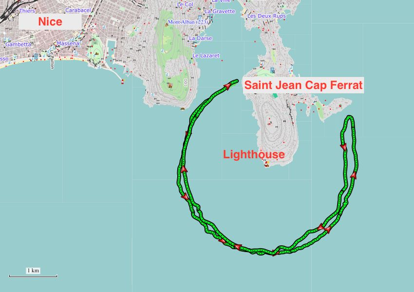
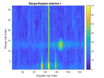
4 AMS JOURNAL NAME

group of 7 CSS within one hour record, we also apply
it to other available incomplete groups of samples.
There are 2 possible groups of 6 consecutive CSS,
3 groups of 5 CSS, etc. This amounts to apply the
DoA algorithm as many times as they are admissible
groups, thereby obtaining multiple estimates of the
spatial distribution of surface current. In the end,
a radial current map with a significantly increased
coverage can be obtained by averaging the individual
maps derived from every single group. Starting with a
minimal size of 3 CSS, there are 15 admissible groups
of consecutive CSS. Note that smaller groups provide
coarser estimates of the covariance matrix hence the
radial current direction. However, they help filling the Fig. 2. Ship trajectory for the antenna pattern campaign
map while higher-order groups ensure more accurate
estimates. Different weights can be attributed to the
latter to favor large groups and increase the accuracy.
We refer to this technique as “temporal stacking”, as
it is a well-known technique in signal processing to
take advantage of redundant samples.

4. Ship calibration of the antenna patterns
a. Standard calibration procedure
 As already mentioned the antenna calibration is a
crucial step for the quality of HFR surface current
measurement. The CODAR SeaSonde manufacturer
provides a specific transponder and a well-established
procedure to perform this calibration with a ship-
borne transmission. The transponder interacts with
the radar receiver to characterize the antenna pattern Fig. 3. Experimental antenna patterns derived from the Sea-
in the practical configuration of the field deployment. Sonde software. The red (blue) thick solid lines show the
The boat describes a circle around the antennas while smoothed measured angular pattern. The magenta (cyan) thin
 solid lines indicate the ideal pattern at the main bearing extrapo-
the HFR system acquires the transponder signal. The lated from the minimum of loop 2 (orange solid line).
exact ship position is tracked with a GPS device and
the track must be traveled clockwise and counter-
clockwise to eliminate some possible bias in time The recorded time series were processed by the
and average the measurements. SeaSonde software to extract the antenna pattern and
 The field campaign for the antenna calibration was were also processed from scratch at the laboratory.
carried over on March, 11, 2020 with a standard Sea- We recall hereafter the main steps of the calibration.
Sonde transponder mounted on the Pelagia boat (In-
stitut de la Mer de Villefranche). The distance was 1. Record the raw I/Q time series (Llv files) on the 3
maintained constant at one nautical mile from the receiver channels when the transmitter is a shipborne
SeaSonde antenna, a short range which is imposed by transponder.
the weak power of the transponder. At this distance 2. Process the received signal in range (fast time)
the geographic situation (peninsula of Cap Ferrat) al- and Doppler (slow time) to obtain Range-Doppler
lows to cover a circular arc from 60◦ to 330◦ NCW. maps. Thanks to the GPS track of the ship, every
The ship trajectory is shown on Figure 2. The boat such map can be associated to an azimuth .
was driven at a speed ranging from 10 km/h to 15 3. Identify the bright spot corresponding to the
km/h which is equivalent to an angular velocity be- ship echo in the Range-Doppler domain and the
tween 4 to 6 degree of arc per minute, well below corresponding Range-Doppler cell. The transponder
the 8.5 knots (15.7 km/h) velocity threshold recom- and the receiver parameters have been set in order to
mended by experimented users (Updyke (2020)) for locate a signal peak in range cells from 10 to 13 and
such measurements. Doppler cells from 35 to 55.

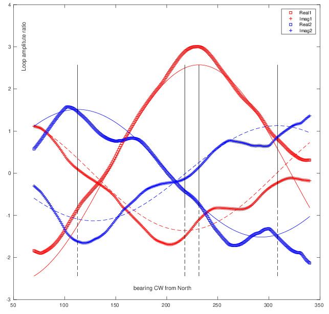
5

4. For each antenna, calculate the complex gain 1 minute within the 256 second duration of each Llv
 1 ( ), 2 ( ), 3 ( ) of each antenna in the direction of file, thereby providing an estimation of the complex
the ship by evaluating the complex Doppler spectrum Doppler spectrum every 30 seconds. The resulting
in the related cell. Ideally, the ship response involves loop amplitude ratio are further interpolated at the
a single cell in the Range-Doppler map. In practice, GPS time scale (1 second). Figure 4 shows an ex-
the ship illuminates a few neighbor cells. The ample of the obtained Range-Doppler maps for the
antenna gain can be chosen as the mean complex first antenna. The positive and negative Bragg lines
Doppler spectrum over these neighbor cells or the are clearly visible together with the zero-Doppler line
complex value where the amplitude is maximum. (fixed echos) and a bright spot around position 90-13
The so-called complex loop amplitude ratios of corresponding to the ship signal.
antennas 1 and 2 are be obtained by normalizing
the ship response by antenna 3 (monopole), that is
 1 ( ) = 1 / 3 and 2 ( ) = 2 / 3 .
5. Perform a sufficient angular smoothing of the
complex loop amplitude ratios to remove the fast
oscillations.

 Figure 3 shows the antenna power patterns (that
is, | 1 ( )| 2 and | 2 ( )| 2 ) obtained with the SeaSonde
software processing of the field measurement after
an angular smoothing over a 10 degrees window and
interpolated with 1 degree steps. A significant de-
viation from the ideal pattern can be observed both
in shape and orientation. The main bearing cannot
be determined without ambiguity as the maximum of
 Fig. 4. Example of Range-Doppler spectra on the three an-
loop 1 does not coincide with the minimum of loop
 tennas (in dB scale). The bright spot around coordinates 90-12
2. The position of the latter is, however, difficult to is due to the ship motion. The zero Doppler ray (central vertical
estimate as it is hidden by a secondary lobe. Based on line) as well as the Bragg lines are clearly visible.
the extrapolation of the edges of the main 2 lobes of
loop 2, the main bearing is found at 212 degree NCW The complex antenna patterns 1 , 2 can be repre-
(versus 207 degree when measured with the magnetic sented in amplitude and phase as:
compass and the mast marker). This bearing value
will be used in the following to characterize the ideal ( ) = ( ) , = 1, 2 (4.4)
pattern of the Ferrat station.
 In the ideal case, the amplitude 1 , 2 coincide with
b. Laboratory calibration the absolute values of the sinus and cosinus function
 The quality of the overall processing is strongly de- around the main bearing and the phases 1 , 2 are
pendent of the windowing process and the integration 0 or 180 degrees. The measured patterns are in the
times which are chosen to perform the range resolu- favorable case slightly distorded versions of the ideal
tion and the Doppler analysis. Each Llv file consists patterns. For simplicity we assume the distorsion can
of 512 sweeps with 4096 samples corresponding to be described in overall phase and amplitude but not
total duration of 256 second. Within each sweep (du- in shape. As suggested in Laws et al. (2010) we use
ration = 0.5 sec), the received I/Q signal is sampled the following parametric form (assuming no constant
at a fast time with 4096 points. Range processing is bias):
obtained using FFT with a Blackman-Harris window.
Among the 2048 available positive frequency bins, 1 ( ) = 1 cos( − 1 ) 1 , 2 ( ) = 2 sin( − 2 ) 2
only the first 32 frequency bins are preserved, corre- (4.5)
sponding to the closest range cells from 1 to about for some tuning coefficients 1 , 2 , 1 , 2 , 1 , 2 .
60 km. This provides range-resolved time series on These parameters can be easily identified by fitting
each antenna at 2 Hz sampling frequency. Doppler the real and imaginary parts of the complex loop am-
spectra are obtained by applying a further FFT on plitude ratios in the form:
these time series. A trade-off between the required
integration time and the necessary update rate was Re ( ) = cos + sin , ( = 1, 2)
 (4.6)
found by processing 7 half-overlapping sequences of Im ( ) = 0 cos + 0 sin , ( = 1, 2)

6 AMS JOURNAL NAME

Comparison of the expressions (4.6) and (4.5) leads 5. Self-calibration of the antenna patterns
to the consistency relations:
 a. Main principle
 0 0
 tan 1 = 11 = 10 , tan 2 = − 22 = − 20 The experimental calibration of the antennas in real
 1 2
 0 0 (4.7) conditions is far from being satisfying both in terms of
 tan = = , ( = 1, 2)
 2 = 2 + 2 + ( 0 ) 2 + ( 0 ) 2 , ( = 1, 2) quality and tractability. The most obvious drawback
 is that it requires time- and money-consuming opera-
 tions. Another uncomfortable aspect of the procedure
 a b 0 (deg) (deg) is the strong assumption that the antenna patterns that
 real 1 -1.6 -2.0 232 -34|-23 2.9 are measured one mile away from the radar still hold
 at longer range, which ignores the shielding by nat-
 imag 1 1.1 0.8 218 ural remote obstacles (islands, coasts, capes,...). We
 real 2 -0.6 1.4 203 -50|-32 1.9 have also seen that the quality of the estimation of
 imag 2 0.7 -0.9 218 the complex gain relies on the choice of several tun-
 Table 1. Estimation of the main bearing ( 0 ) and the ampli- ing parameters in the radar processing (length of the
tudes ( 1 , 2 ) and phases ( 1 , 2 ) of the complex loop amplitude time series to process, tapering window, number of
ratios (4.5) from the fitting coefficients , of equation (4.6) Doppler spectra to average, selection of the ship re-
 sponse in the range-Doppler maps, smoothing of the
 The estimated values for the fitting parameters are angular diagram, etc). Besides, the calibration might
recapped in Table 1. Figure 5 shows the real and imag- be subject to variations in time depending to meteo-
inary parts of the loop amplitude ratios 1 ( ), 2 ( ) rological conditions or drift of electronic devices. To
as a function of the bearing angle together with their avoid the heavy procedure of ship calibration, some
least-square fit (4.6). The black dashed vertical lines other techniques have been proposed in the literature
indicate the different values found for the estimated based on external opportunity sources (see e.g. Fer-
bearing. A running average within a ±40 degree trian- nandez et al. (2003, 2006); Flores-Vidal et al. (2013);
gular window as been preliminary applied to smooth Zhao et al. (2020) for antenna arrays and Emery et al.
the measured complex patterns. By taking the average (2014) for compact systems), provided there is a suffi-
value of the parameters which have a double deter- cient number of ship tracks under the radar coverage.
mination ( 1 , 2 , 1 , 2 ) we can estimate 1 ' 225◦ , We here propose a novel method which does not re-
 2 ' 210◦ , 1 ' −28◦ and 2 ' −41◦ . As seen, the quire any external source and is purely based on the
estimated angles 1 and 2 differ by 15 degree, indi- analysis of the recorded Doppler spectra. The main
cating that the actual patterns of loop 1 and 2 fail to idea is that a proper family of steering vector g ( ) of
satisfy the assumed quadrature relation. the antenna system should cover the eigenvectors of
 the Doppler rays covariance matrix whenever a va-
 riety of DoA are investigated. In other words, when
 performing the SVD decomposition of the covariance
 matrix for a large number of range cells and Doppler
 rays and for the large variety of oceanic patterns en-
 countered on the long-term, the obtained eigenvectors
 should remain within a constrained family given by
 the steering vector. We therefore devise the following
 algorithm for the estimation of the latter.
 (i) We first seek a relevant representation of
 the antenna pattern with the help of a reduced
 set of parameters, X , and we denote g ( ; X ) =
 ( 1 ( ; X ), 2 ( ; X ), 1) the associated steering vec-
 tor. In the following we will keep the same parame-
 terization (4.5) that was used to fit the experimental
 lobe which requires only 6 coefficients. However,
 Fig. 5. Measured (symbols) and fitted (lines) values after
 contrarily to this former case, there is no reference di-
equation (4.6)) for the complex loop amplitude ratios (4.5). The rection for the trial antenna pattern (since the antennas
black dashed vertical lines indicate the different values found for covariance matrix is only sensitive to the relative di-
the estimated bearing. rections of the sources with respect to the antenna
 gains). A directional marker can be obtained from

7

the coastline, which limits the admissible angular do- The Median was preferred to the Mean or the Maxi-
main. We will therefore seek to optimize the antenna mum value of the population which are too sensitive
pattern under the form: to outliers and lead to a noisy and discontinuous de-
 pendence of the cost function on the trial parameters
 1 ( ) = 1 cos( − 1 ) 1 ( ),
 (5.8) X . The optimal set of parameters can then be es-
 2 ( ) = 2 sin( − 2 ) 2 ( ), timated using a classical minimization routine with
 some initial guess on the parameter values.
where ( ) is an angular mask delimitating the max-
imum opening to sea (i.e., a land mask), ( ) = 1 if
 < < and ( ) = 0 otherwise. b. Application to the CODAR station

(ii) Record a long series of range-resolved com- The aforementioned self-calibration procedure was
plex Doppler spectra for each antenna (CSS files) with applied to the SeaSonde data using one full month
the standard integration time (10 min). Assuming a of record (May, 2019). The six parameters of the
constant calibration over the period, this series should cost function were optimized using the minimization
cover at least a few weeks and a variety of oceanic toolbox of Matlab and the ideal pattern parameter as
conditions (hence various current patterns). an initial guess. The obtained antenna patterns are
 summarized in Table 2, together with a recap of the
 (iii) For every nth Doppler ray above some thresh- parameter values for the ideal and experimental lobes
old (depending on the range), calculate the antenna (whenever available). Note that the estimated as well
covariance matrix using an ensemble average over as measured antenna patterns are far from satisfying
the standard duration (typically, 7 CSS files over one the expected quadrature relation between loop 1 and
hour). Perform a SVD of this matrix and store the loop 2, judging from the significantly different values
corresponding eigenvectors 1 , 2 , 3 corresponding obtained for the bearings 1 and 2 which have a
to the 3 eigenvalues 1 , ≥ 2 ≥ 3 . Repeat this oper- discrepancy of about 15 degrees.
ation for every hour of data in the databasis. Stack Figure 6 shows one example of radial map obtained
the available eigenvectors obtained with different with the self-calibrated antenna patterns and their
times, range and Doppler rays in a unique large 3 × comparison with those obtained with the ideal and
 
matrix of vectors ( 1 , 2 , 3 ). This constitutes experimental antenna patterns. The small differences
the reference databasis of eigenvectors for the self- in the amplitude and bearing antenna parameters re-
calibration process. sult in an overall rotation and dilation of the map. It
 (iv) For every set of parameters X characterizing also illustrates the advantage of using temporal stack-
the antenna pattern, evaluate a cost function L ( X ) ing. As seen, this technique significantly improves
defined in the following way. Let us denote g ( ; X ) the coverage of the map of radial current and prevents
the steering vector associated to this trial pattern. For from using interpolation techniques which could in-
 troduce artifacts in the distribution. Note, however,
every ℎ set of eigenvectors ( 1 , 2 , 3 ) and antenna
 that the azimuthal resolution has not been increased
parameters X , one can evaluate a MUSIC factor:
 and is still limited by the geometry of the antenna
 receive array.
 © k g ( ; X )k ª
 ( ; X ) = max ­­ Í ®,
 3 ®
 ( V · g ( ; X )) V 1 2 1 2 1 2
 « =3− +1 ¬ Id. 1 1 212 212 0 0
 (5.9)
where is the chosen number of sources. The main Exp. 2.9 1.9 225 210 -28 -41
idea is that the MUSIC factors ( ; X ) obtained by Self. 1.43 1.43 225.6 205.1 -9.9 -20.9
using the eigenvectors databasis will be amplified if
 Table 2. Estimation of the antenna pattern parameters for the
the trial steering vector ( ; X ) has a good match with
 ideal (Id.), experimental (Exp.) and self-calibrated (Self.) lobes
the actual steering vector one at the detected DoA. at the CODAR station Saint-Jean Cap Ferrat. The angles are given
When using a large databasis, say over one month, in degrees NCW.
one can expect that the variety of encountered oceanic
conditions will allow to sweep all possible bearings.
 The number of sources that can be used in the MU-
To quantify the global increase of the MUSIC factors,
 SIC DF algorithm is, at most, one unity less than the
we selected a criterion based on the median of the
 number of receive antennas. This imposes at most
population. We therefore devised the following cost
 two sources in the case of the CODAR. In principle,
function:
 using two sources instead of one provides a better es-
 L ( X ) = (Median ( ( ; X ))) −1 (5.10) timation of the spatial structure of the radial current,

8 AMS JOURNAL NAME

a) b)

c) d)
 Fig. 6. Examples of radial current maps obtained at the Ferrat station using 1 hour of record (May, 13, 2019, 16:00 UTC) and
the (a) ideal, (b) experimental and self-calibrated (c) antenna pattern. Temporal stacking and one single source have been used in the
DoA algorithm. The effect of stacking is illustrated in (d), where the radial map obtained with the self-calibrated antenna pattern (c)
is recalculated without temporal stacking.

in particular in non-trivial situations when the latter 6. Comparison with drifters
has meandering or vortices leading to multiple DoA
 To assess the respective merits of the different cali-
for a given radial current value. However, using a
 bration methods, we compared the HFR radial surface
two-source DF is very demanding in terms of accurate
 currents with drifters’ measurements obtained during
knowledge of the antenna pattern and level of SNR for
 an experiment conducted in May, 2019. To this aim,
the Doppler rays. The main reason is that the noise we re-calculated the self-calibrated antenna pattern
subspace is very sensitive to a wrong evaluation of using the corresponding month of data. An exam-
the antenna pattern in the azimuthal directions where ple of a typical radial current map seen from this
some of the signal subspace antennas receive a weak station is shown in Figure 6b. The drifter set, used
signal (hence a weak SNR). This produces many er- as ground truth, is part of the dataset collected un-
rors in the estimation of the DoA and therefore many der the IMPACT EU project (IMPACT (2016)) aim-
outliers in the surface current map. The optimal num- ing to provide tools and guidelines to combine the
ber of sources is one unity less than the number of conservation of the marine protected areas with the
antennas having simultaneously a sufficient SNR for development of port activities in the transboundary
all directions. In the case of the SeaSonde of Saint- areas in between France and Italy. The deployment
Jean Cap Ferrat we found that the loop 2 antenna has includes 40 CARTHE-type drifters, biodegradable up
a weak SNR even outside the main lobe of the loop to 85% (Novelli et al. (2017)), released in the open
1 antenna, making a two-source DF estimate prone sea in front of the Gulf of La Spezia (Italy) on May
to errors. We therefore decided to perform the whole 2, 2019 (Berta et al. (2020)). The deployment strat-
azimuthal processing with one single source, which is egy consisted of releasing 35 drifters on a regular
less accurate but more robust than two sources in this grid (about 6km side and 1km step, with some 500
case. Similarly, the self-calibration of the antenna m nesting) in a time window of about 2-3 hours. 5
pattern was realized using a single source in a region more drifters were released in line after passing by
of strong SNR (range cells 7 to 17). the Portovenere Channel, while exiting the Gulf of

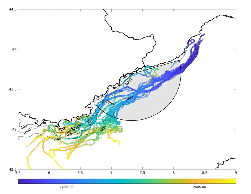
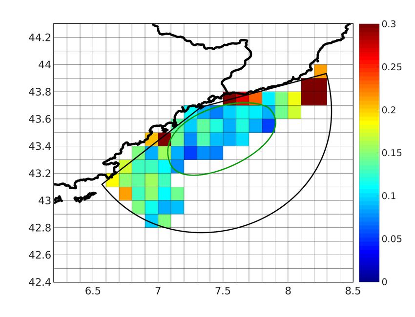
9

La Spezia. The nominal drifter transmission rate is method being at first sight best performing. How-
5 min, GPS transmitters nominal accuracy is within ever, some non-negligible errors are visible in the
10 m, and drifter positions were pre-processed to re- magnitude of the peaks around May, 10 and May,
move outliers. Most of the drifters followed the pre- 15, 2019. To quantify the performances of the dif-
vailing current pattern in the area, represented by the ferent calibration techniques we calculated the main
NC, and moved along the continental margin from statistical parameters of the overall dataset. By con-
the North East to the South West in agreement with catenating the time series from the 40 trajectories,
the general cyclonic circulation of the NW Mediter- we obtained an ensemble of 8090 simulataneous val-
ranean basin. Most of the drifters reached the area ues of HFR and drifter’s radial currents over the en-
of interest, around May 10, and 35 trajectories were tire experiment ( and , respectively).
specifically chosen for the HFR currents assessment From this ensemble of values we calculated the bias
in between May 10 and May 20, wherever a non-void (h − i), the Root Mean Square Error
intersection was obtained with the HFR surface cur- (RMSE=(h[ − ] 2 i) 1/2 ) and the corre-
rent estimates. In order to compare with HFR data, lation coefficient of the linear regression for each of
drifter positions were interpolated on the HFR time the 3 calibration methods. The results are summa-
vector and drifter velocities were projected onto the rized in Table 3. As seen, using the experimental an-
radial direction of the antenna pattern. The surface tenna patterns only marginally improves the accuracy
layer sampled by CARTHE drifters covers the first for the estimated radial currents when compared to the
60 cm of the water column (Novelli et al. (2017)). ideal pattern. However, the use of the self-calibrated
This is consistent with the water layer measured by antenna pattern allows for a significant decrease of
HFR since velocities are vertically averaged down to RMSE (by 3 cm/s) with respect to the ideal pattern.
a depth estimated as /8 , where is the transmitted To better identify the area where the HFR esti-
radar wavelength (Stewart and Joy (1974)), which cor- mates are of lesser quality, we calculated the RMSE
responds approximately to a layer of about 88 cm for in restricted areas corresponding to 0.1 degree bins
the considered HFR operating frequency 13.5 MHz. of longitude and latitude and retained only the grid
CARTHE drifters have low windage, thanks to the flat cells where at least 10 sample points were available
toroidal floater. In addition, their motion is not af- (out of 8090). Figure 9 shows the obtained RMSE in
fected by rectification caused by wind waves, thanks colorscale, superimposed to the map of radar cover-
to the flexible tether connecting the floater and the age. From this refined analysis it turns out that the
drogue; at last, their slip velocity is less than 0.5% accuracy of the HFR estimation is greatly improved
for winds up to 10 m/s (Novelli et al. (2017)). Some in a central zone which can be coarsely delimitated
of these CARTHE drifters reached the area of Toulon by a square area comprised between 7.3-7.9 longitude
in the stream of the NC around May, 19, 2019 (see and 43.3-43.7 latitude. The RMSE obtained by con-
Figure 7) and their data were already compared with sidering all data in this central zone is found to about
the radar estimates from the local HFR stations (a 10 cm/s when using the self-calibrated antenna pat-
WERA bistatic network at 16.15 operating frequency tern, which is 2-3 cm/s lower than the corresponding
(see Guérin et al. (2019))). An excellent agreement RMSE calculated with the ideal or measured antenna
(2-5 cm/s RMSE) was found for the corresponding ra- pattern. Given the magnitude of the radial surface
dial currents (Dumas et al. (2020)), thereby confirm- current (up to 1 m/s) this is a good performance.
ing that the CARTHE are very relevant instruments
to calibrate HFR surface current measurements.
 For the purpose of comparison, the drifter’s veloc- bias RMSE CC
ity were projected on the local radial seen from the ideal 5.7 (8.2) 17.5 (12.8) 0.88 (0.91)
HFR site and the hourly HFR measurements were in- measured 8.1 (2.7) 16.1 (13.6) 0.88 (0.86)
terpolated both in space and time to match the drifter’s self-calibrated 6.1 (3.1) 14.3 (10.2) 0.88 (0.91)
locations. We inspected the HFR velocities obtained
with each of the 3 calibration methods along the indi- Table 3. Overall statistical performances of the HFR radial
vidual drifter trajectories. Figure 8 shows an example current measurements when compared to the 40 drifters. The bias
 and RMSE are given in cm/s and CC is the correlation coefficient.
of such comparison for one trajectory that remained In parenthesis, the same statistical performances on the reduced
entirely within the radar coverage over the duration of area comprised between 7.3-7.9 longitude and 43.3-43.7 latitude.
the experiment. As seen, the dominant inertial oscil-
lations are well captured by the HFR estimates for all
types of antenna calibration with the self-calibration

10 AMS JOURNAL NAME

 Journal of Operational Oceanography, 8 (2), 95–107, doi:
 10.1080/1755876X.2015.1087184, number: 2.

 Berta, M., R. Sciascia, M. Magaldi, and A. Griffa, 2020:
 Drifter deployment in the framework of the IMPACT (Port
 impacts on marine protected areas: transnational coopera-
 tive actions) project. SEANOE, CNR ISMAR. URL https:
 //doi.org/10.17882/72369.

 Berta, M., and Coauthors, 2018: Wind-induced variability in the
 northern current (northwestern mediterranean sea) as depicted
 by a multi-platform observing system. Ocean Science, 14 (4),
 689–710, URL https://doi.org/10.5194/os-14-689-2018.

 Coppola, L., L. Legendre, D. Lefevre, L. Prieur, V. Taillandier,
 Fig. 7. Drifters’ trajectories from May, 10 to May, 20, 2019. and E. D. Riquier, 2018: Seasonal and inter-annual variations
The color scale indicates the running date. The typical radar of dissolved oxygen in the northwestern mediterranean sea
footprint of the Ferrat station is shown with the black arc of circle. (dyfamed site). Progress in Oceanography, 162, 187–201.

 Coppola, L., P. Raimbault, L. Mortier, and P. Testor, 2019: Moni-
7. Conclusion toring the environment in the northwestern mediterranean sea.
 Eos, Transactions American Geophysical Union, 100.
 We have presented in detail the first results of one
SeaSonde CODAR station in the region of Nice to- Dumas, D., A. Gramoullé, C.-A. Guérin, A. Molcard, Y. Our-
gether with the specific processing techniques which mieres, and B. Zakardjian, 2020: Multistatic estimation of
 high-frequency radar surface currents in the region of Toulon.
have been developed at the laboratory. An original Ocean Dynamics, 70 (12), 1485–1503, number: 12 Publisher:
self-calibration technique of the antenna patterns has Springer.
been applied and allows to improve the quality of
the HFR radial currents. The accuracy of the latter Dumas, D., and C.-A. Guérin, 2020: Self-calibration and antenna
 grouping for bistatic oceanographic High-Frequency Radars.
has been assessed with the help of a set of drifters’
 arXiv preprint arXiv:2005.10528.
measurements and the RMSE has been shown to be
diminished by 2-3 cm/s with respect to the HFR es- Emery, B. M., L. Washburn, C. Whelan, D. Barrick, and J. Harlan,
timations based on the ideal or experimental antenna 2014: Measuring antenna patterns for ocean surface current hf
patterns. The strong point of this self-calibration radars with ships of opportunity. Journal of Atmospheric and
 Oceanic Technology, 31 (7), 1564–1582.
procedure is that it does not require any extra ship
campaign nor external sources and is purely based on Fernandez, D. M., J. Vesecky, and C. Teague, 2003: Calibration of
the analysis of the recorded time series which can be hf radar systems with ships of opportunity. IGARSS 2003. 2003
updated at will. The results pertaining to the com- IEEE International Geoscience and Remote Sensing Sympo-
panion HFR station recently installed in Menton will sium. Proceedings (IEEE Cat. No. 03CH37477), IEEE, Vol. 7,
 4271–4273.
be presented in a subsequent work, together with the
vector reconstruction of the radial currents. Fernandez, D. M., J. F. Vesecky, and C. Teague, 2006: Phase
 corrections of small-loop hf radar system receive arrays with
 Acknowledgments. The CODAR SeaSonde sensors ships of opportunity. IEEE Journal of Oceanic Engineering,
of the MIO were jointly purchased by several French Re- 31 (4), 919–921.
search institutions (Université de Toulon, CNRS, IFRE-
MER). Their maintainance has been supported by the na- Flores-Vidal, X., P. Flament, R. Durazo, C. Chavanne, and K.-W.
 Gurgel, 2013: High-frequency radars: Beamforming calibra-
tional observation service “MOOSE” and the EU Interreg tions using ships as reflectors. Journal of Atmospheric and
Marittimo projects SICOMAR-PLUS and IMPACT. Spe- Oceanic Technology, 30 (3), 638–648.
cial thanks go to the office of “Phares et Balises DIRM
Méditerranée” for hosting our installation in Saint-Jean Guérin, C.-A., D. Dumas, A. Gramoullé, C. Quentin, M. Saillard,
Cap Ferrat; the Institut de la Mer de Villefranche for lend- and A. Molcard, 2019: The multistatic HF radar network in
ing the Pelagia boat; D. Mallarino, J-L. Fuda, T. Missamou Toulon. IEEE Radar 2019 Conference, IEEE.
and R. Chemin for assisting with installation and Marcello
 IMPACT, 2016: IMpact of Ports on marine protected areas: Co-
Magaldi for the IMPACT drifters campaign. operative Cross-Border Actions. www.impact-maritime.eu.

References Laws, K., J. D. Paduan, and J. Vesecky, 2010: Estimation and as-
 sessment of errors related to antenna pattern distortion in codar
Bellomo, L., and Coauthors, 2015: Toward an integrated HF seasonde high-frequency radar ocean current measurements.
 radar network in the Mediterranean Sea to improve search and Journal of Atmospheric and Oceanic Technology, 27 (6),
 rescue and oil spill response: the TOSCA project experience. 1029–1043.

11

 Fig. 8. Comparisons of HFR derived radial surface current (dots) with drifters’ measurements (black solid line) for one complete
trajectory. The different colors (red, green and blue) refer to the different antenna patterns which have been used (ideal, experimental
and self-calibrated, respectively).

 Novelli, G., C. Guigand, C. Cousin, E. Ryan, J. Laxage,
 H. Dai, K. Haus, and T. Özgökmen, 2017: A Biodegrad-
 able Surface Drifter for Ocean Sampling on a Massive Scale.
 J. Atmos. Oceanic Technol., 34, 2509–2532, doi:10.1175/
 JTECH-D-17-0055.1.

 Quentin, C., and Coauthors, 2013: HF radar in French Mediter-
 ranean Sea: an element of MOOSE Mediterranean Ocean
 Observing System on Environment. Ocean & Coastal Ob-
 servation: Sensors ans observing systems, numerical mod-
 els & information, Nice, France, 25–30, URL https://hal.
 archives-ouvertes.fr/hal-00906439.

 Quentin, C. G., and Coauthors, 2014: High frequency sur-
 face wave radar in the french mediterranean sea: an ele-
 ment of the mediterranean ocean observing system for the
 environment. 7th EuroGOOS Conference, Oct 2014, Lisboa,
 Portugal, ISBN 978-2-9601883-1-8, 111–118, URL https:
 //hal.archives-ouvertes.fr/hal-01131489.
 Fig. 9. RMSE (in m/s) between self-calibrated HFR currents
and drifter measurements calculated with all available sampling Schmidt, R., 1986: Multiple emitter location and signal parameter
points along the 40 trajectories and binned by 0.1 deg bins in estimation. IEEE transactions on antennas and propagation,
latitude and longitude. The black arc of circle shows the typi- 34 (3), 276–280.
cal radar footprint while the green ellipse delimitates the central
region where the error is smallest. SICOMAR-PLUS, 2018: SIstema transfrontaliero per la si-
 curezza in mare COntro i rischi della navigazione e
 per la salvaguardia dell’ambiente MARino. http://interreg-
 maritime.eu/web/sicomarplus.
Manso-Narvarte, I., E. Fredj, G. Jordà, M. Berta, A. Griffa, A. Ca-
 ballero, and A. Rubio, 2020: 3d reconstruction of ocean ve- Stewart, R. H., and J. W. Joy, 1974: HF radio measurements of
 locity from high-frequency radar and acoustic doppler cur- surface currents. Elsevier, Vol. 21, 1039–1049.
 rent profiler: a model-based assessment study. Ocean Science,
 16 (3), 575–591. Updyke, T., 2020: Antenna pattern measurement guide. Tech.
 rep., Old Dominion University.
Mantovani, C., and Coauthors, 2020: Best practices on high Zhao, C., Z. Chen, J. Li, F. Ding, W. Huang, and L. Fan, 2020:
 frequency radar deployment and operation for ocean current Validation and evaluation of a ship echo-based array phase
 measurement. Frontiers in Marine Science, 7, 210. manifold calibration method for hf surface wave radar doa
 estimation and current measurement. Remote Sensing, 12 (17),
MOOSE, 2008-: Mediterranean Ocean Observing System for the 2761.
 Environment. https://www.moose-network.fr/fr.