Hydrological and physico-chemical dynamics in two Andean streams
←
→
Page content transcription
If your browser does not render page correctly, please read the page content below
Limnetica, 39(1): 17-33 (2020). DOI: 10.23818/limn.39.02
© Asociación Ibérica de Limnología, Madrid. Spain. ISSN: 0213-8409

Hydrological and physico-chemical dynamics in two Andean streams

Alejandro Sosnovsky1,*, Magalí Rechencq1, María Valeria Fernández1, María José Suarez2
and Rodolfo Juan Carlos Cantet2,3
1 Grupo de Evaluación y Manejo de Recursos Ícticos, INIBIOMA, Universidad Nacional del Comahue, CONI-
CET, Quintral 1250, R8400FRF San Carlos de Bariloche, Argentina.
2 Departamento de Producción Animal, Facultad de Agronomía, Universidad de Buenos Aires. Av. San Martín
4453, C1417DSQ Ciudad Autónoma de Buenos Aires, Argentina.
3 INPA, Universidad de Buenos Aires, CONICET. Chorroarín 280, C1427CWO Ciudad de Buenos Aires,
Argentina.

* Corresponding author: alejandro.sosnovsky@comahue-conicet.gob.ar

Received: 16/10/18                                  Accepted: 25/02/19

ABSTRACT
Hydrological and physico-chemical dynamics in two Andean streams
Discharge (Q) is an essential variable to understand how fluvial ecosystems function. To this aim, we assessed the hydrological
and physico-chemical dynamics of two contrasting streams in Andean Patagonia: Casa de Piedra (CP) and Gutiérrez (G). CP
originates in a small lake (0.15 km2) situated at high-elevation, whereas the source of G is a large (17 km2) piedmont lake.
There are other differences between the drainage basins of these streams: CP drainage basin covers 63 km2 and slopes steep
(33.9 m/km), while that of G is bigger (162 km2) and gentler (5.9 m/km). The current research was carried out over a period of
1 year. Variables measured were precipitation and temperature, as well as hydrological data (Q = discharge, EC = electrical
conductivity, water temperature, turbidity and pH). The climate and topography of the region led to 3 distinct hydrological
periods: stormflow, meltflow and baseflow. Discharge presented a clear seasonal pattern with higher values at meltflow, due to
snow melting from the mountains. Stream CP was very flashy (high variation in flow regime), unlike stream G. The greatest
flashiness was observed during the stormflow period. Baseflow was characterised by low values of Q. The temperature of water
fluctuated between the different hydrological periods and between the study streams, whereas pH varied seasonally only. Great
turbidity in the streams was observed during the stormflow period, as a result of high run-off. Throughout the year, the relation
between Q and EC in CP revealed different hydrological flowpaths towards the stream: flows derived from melting snow,
lateral flows through the landscape and groundwater flows. In contrast, EC in stream G was high and constant during the whole
recording period, independently of Q. This indicates that the large headwater lake is its main source of water. This lake clearly
affected the physico-chemical dynamics of stream G. In brief, the current research brought new knowledge into the ecological
aspects of hydrological processes acting on the Andean-Patagonian aquatic ecosystems. On the basis of the results presented
here and on expected future trends, we believe that the hydrological and physico-chemical dynamics of these ecosystems will
be highly affected by climate change.
Key words: Patagonia, discharge, electrical conductivity, hydrological periods

RESUMEN
Dinámicas hidrológicas y físico-químicas en dos arroyos de la región andina
El caudal (Q) es una variable esencial para comprender el funcionamiento de los ecosistemas fluviales. En este trabajo
estudiamos las dinámicas hidrológicas y físico-químicas de dos arroyos contrastantes de la Patagonia, el arroyo Casa de
Piedra (CP) y el Arroyo Gutiérrez (G). El arroyo CP nace en un pequeño lago de altura (0.15 km2), en cambio el arroyo G
nace a partir de un gran lago (17 km2) de piedemonte. Además, existen otras diferencias entre sus cuencas de drenaje: la
cuenca del arroyo CP es pequeña (63 km2) y posee una elevada pendiente (33.9 m/km). En cambio, la cuenca del arroyo G
abarca 162 km2 y su pendiente es más suave (5.9 m/km). El presente estudio se llevó a cabo durante 1 año, relevando datos
18                                                   Sosnovsky et al.

climatológicos (precipitaciones y temperatura) e hidrológicos (Q, conductividad eléctrica (CE), temperatura del agua,
turbidez y pH). El clima y la topografía de la región establecieron 3 períodos hidrológicos distintivos: Precipitaciones, Deshie-
lo y Basal. El Q presentó un claro régimen estacional. Los mayores caudales se observaron durante el período de Deshielo por
causa del derretimiento de las nieves en las montañas. El arroyo CP se comportó como un arroyo muy variable en relación
con el Q, no así el arroyo G. La mayor variabilidad del caudal se observó durante el período de Precipitaciones. El período
Basal se caracterizó por su escaso caudal. La temperatura del agua fluctuó entre los distintos períodos hidrológicos y entre
los arroyos de estudio. En cambio, el pH solo fluctuó estacionalmente. La elevada escorrentía durante el período de Precipita-
ciones trajo aparejado el lavado de los suelos y esto a su vez, una mayor turbidez a los arroyos. En el arroyo CP la relación
entre el Q y la CE revelaría diferentes flujos del agua hacia el arroyo durante el año; flujos provenientes del deshielo, de la
escorrentía y subterráneo. En cambio, en el arroyo G, la EC fue elevada y constante durante todo el período de estudio,
independientemente del caudal; indicando al gran lago en su cabecera como su principal aporte de agua. Este lago influyó
claramente en las dinámicas físico-químicas del arroyo G. Este estudio nos permitió indagar sobre procesos hidrológicos con
importancia ecológica en los ecosistemas acuáticos Andino-Patagónicos. A raíz de nuestros resultados y de las tendencias de
futuro, creemos que las dinámicas hidrológicas y físico-químicas de estos ecosistemas se verán fuertemente afectadas como
consecuencia del cambio climático.
Palabras clave: Patagonia, caudal, conductividad eléctrica, períodos hidrológicos

INTRODUCTION                                                       a strong correlation with total suspended solids
                                                                   (TSS) and Total Phosphorus (TP) (Stubblefield et
Streamflow or discharge (Q) is an essential varia-                 al., 2007) and can thus serve as a good surrogate
ble in the functioning of fluvial ecosystems                       for these variables. Water temperature is another
(Ziemer & Lisle, 1998). These systems are fed by                   key variable determining the metabolism of
rain, ice melt, snowmelt and groundwater, the                      organisms (Gillooly et al., 2001) and pH is very
relative importance of each of these factors vary-                 important both chemically and biologically. As
ing over time and space. Moreover, Q varies over                   with Q, these physico-chemical variables have
time frames ranging from hours and days to                         their own characteristics in streams, and are
seasons and years. The pattern of these variations                 affected by the presence of a headwater lake
is referred to as the flow regime of a stream (Poff                (Gordon et al., 2004). Considering lakes as traps
et al., 1997). Stream discharge and flow regime                    for sediments and nutrients (Parker et al., 2009),
are directly related to the surface area of the                    their effluent streams might buffered physi-
drainage basin it runs through. Thus, the smaller                  co-chemical dynamics.
the drainage basin area, the lower Q and the more                      Fluvial ecosystem dynamics are modulated by
frequent and faster the changes in Q (to be more                   climate. In mountain regions the hydrological
“flashy” sensu Baker et al., 2004). Moreover, the                  regime of these ecosystems can be divided into
hydrological dynamics of fluvial ecosystems are                    three contrasting periods: stormflow, meltflow
directly influenced by the presence of headwater                   and baseflow (Ahearn et al., 2004). The storm-
lakes (Gordon et al., 2004). A lake is a water trap,               flow season runs from the beginning of fall to the
thus hydrography of its effluent stream tends to                   end of winter. The snow falling at high altitudes
be stable over time (Fongers et al., 2012).                        contributes to the formation of a snowpack,
Furthermore, Q and its regime have multiple                        which remains frozen until the meltflow period.
impacts on the physical and chemical characteris-                  The latter begins when the temperature rises in
tics of a stream (Baker et al., 2004).                             spring and ends at the beginning of summer. The
    The study of the physico-chemical properties                   baseflow period begins in the summer and ends at
of water gives us meaningful information on the                    the beginning of the fall season. According to the
characteristics of fluvial ecosystems. For exam-                   updated world map of the Köppen-Geiger climate
ple, electrical conductivity (EC) is generally used                classification, Northern Patagonia is character-
as an estimator of Total Dissolved Solids (TDS),                   ized by a temperate climate with warm and dry
and as an indicator of hydrological processes                      summers (Peel et al., 2007). The regional climate
(Moore et al., 2008). Moreover, turbidity presents                 is largely determined by the Andes (Paruelo et al.,

Limnetica, 39(1): 17-33 (2020)
Hydrology in Andean streams 19
1998), since the north-south distribution of these low in winter and summer. No information is
mountains represents an important barrier for given on its stability (as flashiness), or details as
humid air masses coming from the Pacific Ocean. to how it relates to physico-chemical variables.
Most of the water in these maritime air masses Our main hypothesis is that climate is the
falls on the Chilean side of the Andes, and the air principal moderator of aquatic ecosystems in the
becomes hotter and drier through adiabatic warm- Andean Patagonian region. Thus, as in other
ing when descending the Argentine side. East of mountain regions, we divided the hydrological
the Andes, the amount of rainfall follows a regime of Andean Patagonian streams into three
west-east gradient. From the western slopes to the contrasting periods: stormflow, meltflow and base-
eastern limit of the area (about 60 km), annual flow. Each of these periods should have its own
precipitation drops from 3500 mm to 700 mm. characteristic discharge and physico-chemical
Moreover, the precipitation regime presents dynamics. We selected two streams that have the
marked seasonality, occurring during fall and characteristic sources of the streams in the region:
winter (Paruelo et al., 1998). Within the current Casa de Piedra (CP) and Gutiérrez (G). CP origi-
framework of climate change affecting the nates in a small mountain lake, whereas G arises
region, there are strong indications of significant from a large piedmont lake. In a second hypothe-
warming and decreasing precipitation (Masiokas sis, we predict that the large headwater lake of
et al., 2008), which should have an effect on the stream G induces a buffer effect on the hydrologi-
aquatic ecosystems. cal and physico-chemical dynamics of the stream,
Andean rivers and streams have been under and its fluvial dynamics displays greater stability
study for over 30 years now (Modenutti et al., than CP. The first goal of the current research is to
1998), and work carried out in the region has describe the hydrological dynamics of these two
revealed the oligotrophic character of these fluvi- streams. A second objective is to characterize the
al ecosystems (Pedrozo et al., 1993). Diverse temporal dynamics of temperature of water, EC,
authors have studied anthropic (Miserendino et pH and turbidity, and their possible relations to the
al., 2016) and natural (Temporetti, 2006; Lalle- hydrological regime.
ment et al., 2016; Williams Subiza & Brand,
2018) elements that have affected Andean drain- MATERIALS AND METHODS
age basins, and consequently, their fluvial
ecosystems. Recent research has revealed the Area of study
dynamics of organic matter (García et al., 2015b;
Díaz Villanueva et al., 2016; García et al., 2018). The research was conducted at the catchments of
Nevertheless, studies that focus on Q are scarce the streams Casa de Piedra (41° 07’ 30.11'' S 71°
(Barros & Camilloni, 2016), despite the ecologi- 27’ 13.16'' O) and Gutiérrez (41° 09’ 36.18'' S 71°
cal importance of this variable. Andean streams 24’ 37.19'' O), both located in Nahuel Huapi
of Northern Patagonia display a discharge highly National Park, Patagonia, Argentina (Fig. 1). The
dependent on the amount of snow, and then by yearly average of air temperature is 8.3 °C and
glacier melt. This is due to the mild environmen- annual precipitation is 940 mm. This region is
tal conditions and low elevation of Northern Pata- dominated by a mixture of crystalline igneous,
gonian Andes, which limit the effects of glaciers volcanic and plutonic rocks; pyroclastic rocks are
to relatively small ones on the highest peaks and of secondary importance, and metamorphic and
volcanoes along the mountain range (Lliboutry, sedimentary rocks are present in minor quantities
1998). Limnological studies are based on Q data (Pedrozo et al., 1993). Glacial drift and alluvial
measured over a relatively long time interval, and outwash deposits predominate in the valley
characterise the hydrological regime of Ande- bottoms. The area was glaciated extensively and
an-Patagonian streams only in relation to yearly repeatedly during the late Pleistocene (Flint &
climate seasonality by displaying a bi-modal Fidalgo, 1964). The soils are classified as Andis-
pattern. That is, Q is high in autumn and spring ols, which are characterized by high capacity to
due to rainfall and snowmelt, respectively, and is stabilize organic matter, to store water and to
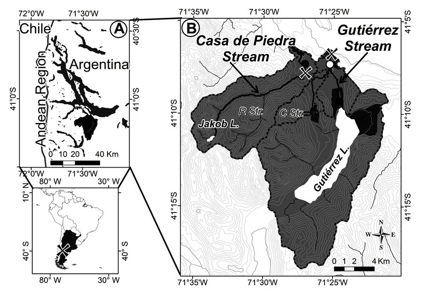
Limnetica, 39(1): 17-33 (2020)20 Sosnovsky et al. Figure 1. a) Nahuel Huapi National Park; the study area is shaded in black. b) Study area, Catchments of Casa de Piedra and Gutiérrez streams. Curves represent 100 m slope on the terrain. Populated zones are shown in grey, crosses indicate sampling sites, black circles indicate the Limnigraphic stations and white circle indicate the rain meter location. R Str. and C Str., Rucaco and Cascada streams. a) Parque Nacional Nahuel Huapi, el área de estudio está sombreada en negro. b) Área de estudio, Cuencas de drenaje de los arroyos Casa de Piedra y Gutiérrez. Las curvas representan un desnivel de 100 m. En gris se indican las zonas pobladas, las cruces indican los sitios de muestreo, los círculos negros indican las ubicaciones de los limnígrafos y el círculo blanco indica la ubicación del pluvió- metro. R Str. y C Str., arroyos Rucaco y Cascada. retain phosphorous (Satti et al., 2003). They also The seasonal concentration of TP is 3.4 μg/l on have a high pH buffering capacity. The drainage average (Diaz et al., 2007). G has only one afflu- basins of both streams are very different from ent (the Cascada stream) whose drainage basin each other, despite of their proximity. In the case covers 12.5 km2. G flows 9 km through a wide, of CP, the catchment covers 63 km2 and the gently sloped valley (5.9 m/km). Its riverbanks stream originates in lake Jakob, a deep (25 m are extensively colonised by the exotic crack maximum depth), small (0.15 km2), ultra-olig- willow, Salix fragilis, and it runs through a series otrophic (1-3 μg/l TP), high altitude lake, situated of populated sections of a city (San Carlos de at 1550 m a.s.l. (García et al., 2015a) (Fig. 1). The Bariloche). In addition, the products from two only affluent is the Rucaco stream having its salmon farms are emptied into its waters. source in high marshlands. CP flows 19.7 km through a steep V-shaped valley (slope: 33.9 Sampling strategy and data collection m/km) from its source until close to its mouth. The CP drainage basin is still pristine, with the The study was carried out over one year, from major human activity being hiking. The vegeta- 21-3-2014 to 20-3-2015. This period was divided tion includes Nothofagus pumilio, and the ever- into 3 hydrological periods: stormflow, meltflow green tree species Nothofagus dombeyi and and baseflow. The stormflow extended from the Austrocedrus chilensis in the low catchment. In beginning of the study up to mid-September contrast, the catchment of G is larger (162 km2), (15-9-2014). The meltflow period followed, and the stream originates in lake Gutiérrez. This ending at the beginning of December lake occupies 11 % of the catchment valley: it is (5-12-2014), Finally, baseflow occurred from deep (111 m maximum depth) and large (17 km2). December 6, 2014 to March 20, 2015. The start- Limnetica, 39(1): 17-33 (2020)
Hydrology in Andean streams                                           21
ing points of the meltflow and baseflow periods
were determined by a marked decrease in precipi-
tation in the drainage basin, and the EC dynamics
in CP. The dynamics of EC from mountain
streams displays a gradual decrease throughout            The variable q is the mean daily flow whereas
meltflow (Drever & Zobrist, 1992; Sueker et al.,      n is the number of observations. This index
2000), reaching its lowest level just before the      measures oscillations in discharge relative to
beginning of baseflow (Ahearn, personal commu-        total discharge. Thus, it is a dimensionless meas-
nication to the first author). The Provincial Water   ure ranging between 0 and 2 (Fongers et al.,
Department provided the data on precipitations        2012). A value of 0 represents an absolutely
and Q. Daily precipitation records were obtained      constant flow; increased R-B index values
with a rain meter (Fig. 1) and do not differentiate   indicate increased flashiness of streamflow. As
between rain or snow. Discharge data were aver-       such, the index appears to provide a useful char-
age daily records from two limnigraphic stations.     acterization of the way watersheds process
These stations were set to estimate the pressure of   hydrological inputs into their streamflow
the water column each 30 minutes and store the        outputs. The index may be calculated annually or
information on a hard disk. Every 2 months data       seasonally (Baker et al., 2004).
were collected, and the corresponding hydromet-
ric gauging was performed. The limnigraphic           Data treatment
station for CP is located close to its mouth, while
for the stream G is located at its source (Fig. 1).   Data on the average daily Q were transformed to
The Q value for G at our sampling site was            normality by the Box-Cox procedure as suggest-
estimated from the sum of Q at its source plus Q      ed by Peltier et al. (1998). The transformed
for the Cascada stream. We determined Q for           records were then analyzed with a fixed effects
Cascada using the Drainage-Area Ratio method          two-way linear model with interaction. Main
(Emerson et al., 2005), taking the specific daily     effects were hydrological period (3 levels) and
value of Q for the nearby CP stream. Specific         stream (2 levels). PROC MIXED of SAS (SAS
discharge was defined as discharge per unit area.     Institute Inc., 2013) was employed to account for
The National Meteorological Service provided          heterogeneous variances due to stream.
average daily air temperatures.                           The Cox and Stuart (1955) test was used to
    We measured the following stream water            analyze trends in Q from the different hydrologi-
variables: turbidity with a Velp turbidimeter, and    cal periods. This test allows verifying whether a
temperature, EC compensated to 25 °C and pH           variable displays a monotonical trend. The null
with an Oakton probe. Sampling was conducted          hypothesis is that the data shows no trend. The
twice weekly during the morning hours. This           test behaves similarly to the sign test for two
frequency was increased whenever precipitation        independent samples (Daniel, 1978).
was forecasted by taking daily samples before,            In addition, we studied the relationship
during and after the precipitation event (Casson      between discharge and environmental variables
et al., 2012; Tate & Singer, 2013). Hence             during each hydrological period and carried out a
sampling frequency varied between 8 and 15            cross-correlation analysis. The methodology is
samples per month.                                    widely used to analyze the linear relationship
                                                      between input and output signals in hydrology
Data processing and analysis                          (Larocque et al., 1998). In our research, the input
                                                      signals were the precipitation and air tempera-
Variability of discharge                              ture, and the output signal was the river discharge
                                                      of CP and G. Cross-correlations are represented
The stream flashiness was measured by the Rich-       by a cross-correlogram. The maximum amplitude
ards-Baker (R-B) index (Baker et al., 2004),          and the lag value of the cross-correlogram
whose formula is as follows:                          provide information on the delay, which indicates

                                                                                Limnetica, 39(1): 17-33 (2020)
22 Sosnovsky et al. Figure 2. Left panels: a) Temperature, c) Precipitation, e) Casa de Piedra stream hydrograph and g) Gutiérrez stream hydrograph. e) and g) R-B index values are shown on the different hydrological periods. Right panels: box-plot of the same data. Data is divided into 3 hydrological periods, Stormflow (St) (n = 179), Meltflow (Me) (n = 81) and Baseflow (Ba) (n = 105). The boundary of the box closest to zero indicates the 25th percentile, a line within the box marks the median, and the boundary of the box farthest from zero indicates the 75th percentile. Whiskers indicate the range. f) and h) Letters (a, b, c, d and e) represent significantly differences (P < 0.05) in Discharge from the interaction between streams x periods. Paneles izquierdos: a) Temperatura, c) Precipitaciones, e) Hidro- grama del arroyo Casa de Piedra, g) Hidrograma del arroyo Gutiérrez. e) y g) Se muestran los valores de los índices R-B para los diferentes períodos. Paneles derechos: representa el mismo conjunto de datos en diagramas de cajas. Los datos están divididos en los 3 períodos hidrológicos, Precipitaciones (St) (n = 179), Deshielo (Me) (n = 81) y Basal (Ba) (n = 105). El límite del cuadro más cercano a cero indica el percentil 25, una línea dentro del cuadro marca la mediana y el límite del cuadro más alejado de cero indica el percentil 75. Los bigotes indican el rango. f) y h) Las letras (a, b, c, d y e) representan diferencias significativas del caudal (P < 0.05) de la interacción arroyos x períodos hidrológicos. Limnetica, 39(1): 17-33 (2020)
Hydrology in Andean streams                                                  23
the time of the pulse transfer to the stream. The       Table 1. Hydrological variables of the study streams. Values
                                                        were obtained from a daily temporal scale (n = 365). Discharge
statistical analysis of discharge included the          (Q), Specific Discharge (Q sp.). Variables hidrológicas de los
stream x period interaction, and the linear covari-     arroyos de estudio. Los valores fueron obtenidos a partir de
ates temperature and rainfall nested within the         una escala temporal diaria (n = 365). Caudal (Q), Caudal
interaction. Again, a heterogeneous residual            específico (Q sp.).
variance was fitted to the model CP displayed
more variability than G.
    To quantify the relation between Q and the                         Q
                                                                                   Q         Q       Q sp. Annual
physico-chemical variables of the streams, we             Stream     Annual
                                                                                  max.      min.       average
                                                                     Average
carried out Spearman correlations. Physi-
co-chemical data was analyzed with the two-fac-                                  m3/s                 m3.s-1.km-2
tor interaction model with heterogeneous                 Casa de
                                                                       3.220     16.500 0.550            0.051
variance as discussed before.                             Piedra
                                                         Gutiérrez     3.855      9.920    1.787         0.024
RESULTS

Climate and hydrology                                   higher in CP (CP r (max) = 0.35 versus G r (max)
                                                        = 0.19). After a rainfall the maximum value of Q
Air temperature and precipitation in the study          was reached the next day for CP, whereas Q
area were typical of the temperate climate in the       peaked 3 to 4 days later in G (Fig. 3a). These
region. Average annual air temperature was 8.7          differences in the relationship between Q and
°C, with the lowest value recorded during storm-        precipitation are well noticed in the hydrograms,
flow (Fig. 2a). Air temperature increased evenly        where the variability in discharge is considerably
during meltflow. On average, the highest temper-        higher in CP than in G (Fig. 2e, g). For CP in the
ature was recorded during baseflow. Annual              latter period discharge did not showed any trend
precipitation was 1092 mm , with 79 % occurring         (P (K ≤ 34│82; 0.5) = 0.1507), whereas in G the
during the stormflow period (Fig. 2d). The melt-        discharge evidenced a tendency to increase (P (K
flow and baseflow periods accounted for 19 %            ≤ 5│82; 0.5) < 0.0001). Notwithstanding this, the
and 2 % of total precipitation, respectively.           highest value of Q was observed at other time
    The Q regime and its associated variables           than stormflow (Fig. 2f, h) even though the period
differed annually between the two streams (Fig.         displayed the highest records of precipitation and
2e, g; Table 1). Annual average Q was higher for G      stream flashiness.
(F = 129; P < 0.0001; d.f. = 1), although the specif-       During meltflow the temperature, but not the
ic Q was not (F = 14928; P < 0.0001; d.f. = 1). The     precipitation, had a positive relationship with Q
most extreme values of Q were observed at CP.           for both streams (Fig. 3b; Table 2b; CP; t = 4.67;
These differences highlight the marked temporal         P < 0.001, d.f. = 356; G; t = 4.98; P < 0.001, d.f.
fluctuation of Q for CP, whereas G showed greater       = 356). The correlation was sizeable for both
stability in the values of Q. The annual R-B indices    streams (CP r (max) = 0.74; G r (max) = 0.68),
were 0.16 for CP and 0.04 for G, indicating that the    and the delay times were short (1 day). Compar-
average day-to-day fluctuations of streamflow           ing the meltflow period with the previous one,
were 16 % and 4 %, respectively.                        stream flashiness was almost the same in G but of
    Moreover, the hydrological regime of the            lower intensity in CP (Fig. 2e, g). Also, the
streams differed between the stormflow, melt-           largest discharge was observed for both streams
flow and baseflow periods. During stormflow,            during meltflow (Fig. 2f, h).
precipitation was positively correlated to Q in             Contrary to the observations in meltflow and
both streams (Fig. 3a; Table 2a; CP: t = 7.13; P <      stormflow, neither precipitation nor temperature
0.001; d.f. = 356; G: t = 2.77; P = 0.0059; d.f. =      were positively correlated to discharge during the
356). The correlation between precipitation and         baseflow period (Fig. 3c; Table 2c). The effects
discharge differed between streams and was              of the scarce precipitations with high tempera-

                                                                                        Limnetica, 39(1): 17-33 (2020)
24 Sosnovsky et al. Figure 3. Cross-correlations between precipitation-discharge (left panels) and air temperature-discharge (right panels) of Casa de Piedra (CP) and Gutiérrez (G) streams in the three hydrological periods. The lags for the maximum r are given for both streams in the stormflow period (left panel) and in the meltflow period (right panel). Correlaciones cruzadas entre las precipitaciones y el caudal (panel izquierdo) y la temperature del aire y el caudal (panel derecho) de los arroyos Casa de Piedra (CP) y Gutiérrez (G) para los 3 períodos hidrológicos. El período de retraso para los mayores r se muestra para el período de Precipitaciones (panel izquierdo) y para el período de Deshielo (panel derecho). tures during baseflow give raise to a negative Physico-chemical dynamics relationship between air temperature and discharge in both streams (CP; t = -2.70; P = Air and water temperatures were closely related 0.0073, d.f. = 356; G; t = -2.56; P = 0.0109, d.f. = throughout the observation period (Fig. 2a, 4a). 356). The Q values and variabilities for CP and G Hence, there were differences in water tempera- presented the lowest values from the whole ture for both streams among the three hydrologi- recording time (Fig. 2e-h). For G, the difference cal periods (Fig. 4b, c). Only during meltflow in Q between baseflow and stormflow was not water temperatures at CP and G were positively significant (Fig. 2h). Also, it was clearly observed correlated with discharge (Fig. 5a, b). In addi- a downward trend in the values of Q for both tion, water temperature at CP was 3 °C colder streams (CP, P (K ≤ 0│40; 0.5) < 0.0001; G, P (K than at G (Table 3). ≤ 0│40; 0.5) < 0.0001). A different picture emerges when comparing Limnetica, 39(1): 17-33 (2020)
Hydrology in Andean streams                                                                25
Table 2a-c. Level of significance (P) of the cross-correlations analysis (r) between Discharge of the study streams and the climatic
variables in the three hydrological periods (lag from 0 to 15 days). a) Stormflow, b) Meltflow and c) Baseflow. Casa de Piedra (CP);
Gutiérrez (G). Nivel de significancia (P) de las correlaciones cruzadas (r) entre el Caudal de los arroyos de estudio y las variables
climatológicas en los tres períodos hidrológicos (retraso de 0 a 15 días). a) Precipitaciones, b) Deshielo y c) Basal. Casa de Piedra
(CP); Gutiérrez (G).

                            a) Stormflow period
                           Lag            Discharge-Precipitacion      Lag        Discharge-Temperature
                          (days)    rCP       PCP      rG        PG   (days)      rCP      PCP     r         PG
                            0      0.29     0.0001 0.12 0.1056         0       -0.15 0.0477 -0.31         0.0000
                            1      0.35     0.0000 0.17 0.0222         1       -0.13 0.0911 -0.29         0.0001
                            2      0.31     0.0000 0.16 0.0288         2       -0.15 0.0418 -0.32         0.0000
                            3      0.31     0.0000 0.19 0.0102         3       -0.14 0.0563 -0.33         0.0000
                            4      0.30     0.0001 0.19 0.0113         4       -0.13 0.0987 -0.34         0.0000
                            5      0.23     0.0027 0.17 0.0274         5       -0.14 0.0588 -0.36         0.0000
                            6      0.20     0.0085 0.14 0.0742         6       -0.16 0.0389 -0.37         0.0000
                            7      0.24     0.0013 0.14 0.0636         7       -0.17 0.0230 -0.38         0.0000
                            8      0.23     0.0020 0.11 0.1489         8       -0.19 0.0118 -0.41         0.0000
                            9      0.18     0.0163 0.06 0.4541         9       -0.20 0.0085 -0.42         0.0000
                           10      0.14     0.0620 0.04 0.6151        10       -0.19 0.0155 -0.42         0.0000
                           11      0.17     0.0243 0.07 0.3963        11       -0.15 0.0488 -0.39         0.0000
                           12      0.12     0.1096 0.06 0.4640        12       -0.13 0.0868 -0.36         0.0000
                           13      0.09     0.2360 0.05 0.5505        13       -0.10 0.2147 -0.35         0.0000
                           14      0.13     0.1063 0.05 0.4864        14       -0.06 0.4828 -0.34         0.0000
                           15      0.13     0.0930 0.06 0.4452        15        0.02 0.7873 -0.33         0.0000

                            b) Meltflow period
                           Lag Discharge-Precipitacion                 Lag     Discharge-Temperature
                          (days)  rCP    PCP      rG     PG           (days)    rCP     PCP     rG          PG
                             0   -0.29 0.0095 -0.33 0.0029               0     0.66 0.0000     0.63       0.0000
                            1    -0.32 0.0044 -0.31 0.0057               1     0.74 0.0000     0.68       0.0000
                            2    -0.34 0.0024 -0.33 0.0033               2     0.73 0.0000     0.67       0.0000
                            3    -0.31 0.0063 -0.30 0.0076               3     0.64 0.0000     0.60       0.0000
                            4    -0.25 0.0315 -0.26 0.0223               4     0.54 0.0000     0.52       0.0000
                            5    -0.13 0.2689 -0.17 0.1424               5     0.43 0.0001     0.46       0.0000
                            6    -0.13 0.2517 -0.17 0.1416               6     0.37 0.0011     0.43       0.0001
                            7    -0.12 0.2949 -0.18 0.1287               7     0.30 0.0101     0.39       0.0005
                            8    -0.02 0.8867 -0.12 0.3326               8     0.16 0.1809 0.32           0.0063
                            9    0.08 0.5150 -0.03 0.8149                9     0.04 0.7549 0.24           0.0455
                            10   0.11 0.3452 0.03      0.8131           10     -0.07 0.5687 0.16          0.1878
                            11   0.07 0.5736 0.01      0.9126           11     -0.14 0.2610 0.12          0.3244
                            12   0.04 0.7363 0.00      0.9929           12     -0.17 0.1634 0.12          0.3201
                            13   -0.04 0.7355 -0.05 0.6730              13     -0.11 0.3718 0.17          0.1782
                            14   -0.15 0.2407 -0.10 0.4037              14     -0.01 0.9247 0.23          0.0669
                            15   -0.24 0.0570 -0.15 0.2414              15     0.03 0.8134 0.26           0.0352

                            c) Baseflow period

                           Lag Discharge-Precipitacion                 Lag Discharge-Temperature
                          (days) rCP    PCP       rG   PG             (days) rCP     PCP    rG    PG
                             0   0.03 0.7237 0.01 0.9422                 0   -0.14 0.1492 -0.15 0.1152
                             1   0.06 0.5591 0.01 0.9437                 1   -0.14 0.1461 -0.17 0.0793
                             2   0.06 0.5681 0.04 0.6918                 2   -0.14 0.1662 -0.17 0.0875
                             3   0.03 0.7753 0.02 0.8193                 3   -0.19 0.0583 -0.20 0.0428
                             4   0.09 0.3523 0.08 0.4328                 4   -0.21 0.0339 -0.20 0.0429
                             5   0.17 0.0977 0.14 0.1794                 5   -0.21 0.0318 -0.20 0.0450
                             6   0.14 0.1590 0.12 0.2396                 6   -0.21 0.0409 -0.21 0.0384
                             7   0.11 0.2836 0.12 0.2450                 7   -0.24 0.0198 -0.25 0.0145
                             8   0.09 0.3557 0.12 0.2484                 8   -0.26 0.0097 -0.27 0.0068
                             9   0.10 0.3115 0.11 0.2829                 9   -0.28 0.0049 -0.30 0.0027
                            10   0.12 0.2490 0.10 0.3235                10   -0.27 0.0086 -0.30 0.0034
                            11   0.09 0.3677 0.09 0.3793                11   -0.25 0.0149 -0.30 0.0039
                            12   0.07 0.4997 0.08 0.4314                12   -0.26 0.0116 -0.30 0.0033
                            13   0.08 0.4543 0.09 0.4142                13   -0.28 0.0061 -0.31 0.0031
                            14   0.16 0.1317 0.16 0.1296                14   -0.29 0.0050 -0.30 0.0041
                            15   0.17 0.1174 0.15 0.1503                15   -0.29 0.0064 -0.30 0.0042

                                                                                                                   Limnetica, 39(1): 17-33 (2020)
26 Sosnovsky et al.
Table 3. ANOVA results from the comparison of the physico-chemical variables between the study streams. Average values,
maximum and minimum in brackets (n = 113, except pH data values n = 100). Resultados de los ANOVA de las comparaciones de las
variables físico-químicas entre los arroyos de estudio. Valores promedio, máximos y mínimos entre paréntesis (n = 113 excepto para
los datos de pH n = 100).
Casa de
Gutiérrez df F-value P-value
Piedra
Temperature (°C) 6.3 (1.3-16.3) 9.5 (5.7-16.8) 1 145.72 < 0.0001
Electrical
42 (22-65) 74 (69-80) 1 995.76 < 0.0001
Conductivity (µs/cm)
pH 7.3 (6.3-8.1) 7.3 (6.4-7.8) 1 0.35 0.5574
Turbidity (NTU) 0.8 (0-20.4) 2.4 (0-48.0) 1 6.48 0.0116
Figure 4. Left panel: Temporal variation of the physico-chemical variables in Casa de Piedra (CP) and Gutiérrez (G) streams. Middle
and right panels: box-plots of the same data. The boundary of the box closest to zero indicates the 25th percentile, the line within the
box marks the median, and the boundary of the box farthest from zero indicates the 75th percentile. Whiskers indicate the 10th and
90th percentiles. For a given stream, box-plots with the same letter (a, b or c) are not significantly different (ANOVA, P < 0.05). EC:
Electrical conductivity, St: Stormflow, Me: Meltflow and Ba: Baseflow. The Y axis in graphs j), k) and l) has 2 segments for better
visualisation of the data. Panel izquierdo: Variación temporal de las variables físico-químicas en los arroyos Casa de Piedra (CP) y
Gutiérrez (G). Los paneles del centro y derechos representan el mismo conjunto de datos en diagramas de caja. El límite de la casilla
más cercana a cero indica el percentil 25, una línea dentro del cuadro marca la mediana y el límite del cuadro más alejado de cero
indica el percentil 75. Los bigotes indican el percentil 10 y 90. Para cada arroyo, los diagramas de caja con la misma letra (a, b o c)
no son significativamente diferente entre sí (ANOVA, P < 0.05). EC: Conductividad eléctrica, St: Precipitaciones, Me: Deshielo y Ba:
Basal. El eje Y posee 2 segmentos para una mejor visualización de los datos en los gráficos j) k) y l).
Limnetica, 39(1): 17-33 (2020)Hydrology in Andean streams 27
the electric conductivities of both streams. The observed values during meltflow (Fig. 4e). A
EC of CP was significantly less than the one from sharp decrease in EC was observed during rainy
G (Table 3). At CP, EC was relatively high during days of the stormflow period. Whereas during
stormflow and baseflow, with the lowest meltflow EC tended to decrease over time, the
Figure 5. Spearman correlation between discharge and physico-chemical variables in the different hydrological periods. Stormflow: ∆,
Meltflow: * and Baseflow: -. Only correlations with P ≤ 0.05 are shown. Values in bold are statistically significant at P ≤ 0.01; those in
italics are statistically significant at P ≤ 0.0001. EC: Electrical Conductivity. Panels g) and h) have different scales in their Y axes. Note the
difference between axes X for each stream. Correlación de Spearman entre el caudal de los arroyos y las variables físico-químicas en los
diferentes períodos hidrológicos. Precipitaciones: ∆, Deshielo: * y Basal: -. Se muestran solamente las correlaciones con P ≤ 0.05. Los
valores en negrita son estadísticamente significativos a P ≤ 0.01, aquellos en itálicas son estadísticamente significativos a P ≤ 0.0001. EC:
Conductividad eléctrica. Los gráficos g) y h) poseen diferentes escalas en sus ejes Y. Notar la diferencia en los ejes X de ambos arroyos.
Limnetica, 39(1): 17-33 (2020)28 Sosnovsky et al.
trend was reversed during the next period (Fig. ones recorded at G remaining relatively constant.
4d). High values of Q corresponded to low EC It was clear that the differences in physico-chemi-
values in the EC-Q relationship in CP, and we cal dynamics were associated with the morpholo-
were able to distinguish three concave up curves gies at catchment.
associated with each hydrological period (Fig. The streams CP and G fit in Haines’ et al.
5c). In contrast, conductivity remained high and (1988) classification of river regimes within
constant in G during all recording time (Fig. 4d) Group 14, which are characterized by a peak
though no significant differences were found during early to middle spring. The highest Q in
among hydrological periods (Fig. 4f). both streams occurred during meltflow, a fact that
Neutral pH values were observed (some being concurs with the positive correlation between air
slightly alkaline) with no significant differences temperature and Q, thus highlighting that melting
between streams (Table 3). Conversely, there snow is the principal source of water for these
were significant differences for pH among hydro- streams. Intermediate Q values were found
logical periods. The pH was alkaline during during stormflow, being more evident in CP due
stormflow, and the values decreased during to the high positive relationship observed
recording time being neutral at the end of obser- between precipitation in the catchment and the
vation at baseflow. We detected significant values of Q. In contrast, the lake acted as a water
differences in pH between baseflow and the other trap in the catchment of G. Thus, the lake stored
two periods (Fig. 4h, i). much of the rainwater during stormflow to
Highest values in average and variability of release them later on during the following
water turbidity were recorded during stormflow periods. The marked seasonality of Q, with the
(Fig. 4k, l). Moreover, we observed high values highest values during the snowmelt season, was
of water turbidity that were in agreement with also observed in other mountains regions (Likens
discharge (Fig. 5g, h). The value of water turbidi- et al., 1967; Brown et al., 2003).
ty decreased during meltflow and reached a mini- Flashiness represents the response of the
mum during baseflow (Fig. 4k, l). We observed stream to many factors in the watershed. The R-B
low values of water turbidity during meltflow and indices were 0.16 and 0.04 for CP and G, respec-
baseflow, generally below 1 NTU. Turbidity was tively. The greater stability of the regime in Q for
significantly low at CP (Table 2). G can be explained by the flow regulation (Baker
et al., 2004) induced by the large headwater lake.
DISCUSSION AND CONCLUSIONS Moreover, the difference in catchment size
between CP and G also explained the differences
We recorded discharge and physico-chemical in R-B indices. Small catchments are characterized
dynamics in the Northern Patagonia Andean by steep slopes and high stream density. As a
streams CP and G during a year under normal consequence, small catchments have flashier
climate conditions. The lowest Q was observed streams than large catchments (Baker et al., 2004).
during the baseflow period, whereas intermediate Additionally, the catchments of CP and G present
values of Q occurred during stormflow to rise to rocky soils or bare grounds from 1500 m a.s.l. In
the highest observed Q during meltflow. The case of CP, the percentage of bare ground repre-
increase in Q was associated to precipitation in sents 30 % of the total catchment area (Queimal-
the catchment area during stormflow, and to air iños et al., 2012). All these characteristics favour
temperature during meltflow. Moreover, we high- superficial or sub-superficial run-off during storm
lighted the principal differences in the physi- events, thus increasing the R-B index. This index
co-chemical characteristics of both streams. Max- at CP was similar to values from Alpine streams.
imum values of turbidity, conductivity and water Holko et al. (2011) studied the flashiness of
temperature were observed in G. We have also Austrian and Slovak streams and found average
found a clear-cut difference in EC dynamics values of 0.18 and 0.15, respectively. These
between the two streams, with those values authors conclude that the main variables affecting
obtained at CP fluctuating markedly, while the the RB-index are the geology and the size of water-
Limnetica, 39(1): 17-33 (2020)Hydrology in Andean streams 29
shed. Conversely, Fongers et al. (2012) suggested 1993). The soils in the catchments of both
that the main factors influencing R-B index were streams have a pH of around 6 (Satti et al., 2007),
the size and the use of the watershed. a level at which retain H+. Therefore, our results
The dynamics of the variable EC is an indica- suggest that during stormflow rainwater reaching
tion of water flowpaths to a fluvial ecosystem the streams as superficial or sub-superficial
(Moore et al., 2008). In stream CP we observed run-offs will be slightly alkalized by the soil,
three different EC-Q curves; one for each hydro- whereas the pH decreases during the following
logical period. At the same time during stormflow meltflow. This observation is in line with the
Q peaked while EC dropped to a minimum. Thus, naturally acidic characteristics of snow; the
there was a high run-off as a large amount of water decrease in pH of streams and lakes during snow-
runs fast into the stream with little interaction with melt is a known process which has been studied
the land ecosystem. In the Melt season, we in other mountain regions (Jeffries et al., 1979;
observed Q at the highest and EC at the lowest, Galloway et al., 1987). During baseflow, the pH
which indicates that water in the river largely of the stream water was neutral. We did not carry
results from melting snow in the uplands and is out any studies on the groundwater in the current
depleted of TDS (Ahearn et al., 2004). The down- research, and therefore have no information as to
ward shift of the EC-Q curve over time reflects the its properties during the recording period. How-
progressively upward shift of run-off source areas ever, measurements taken in the water from a
associated with the rising snow line. This increase spring close to the streams had pH close to 6 and
in elevation of the source areas for snowmelt EC near the level of 100 µS/cm (personal obser-
run-off would be expected to progressively vations of the first author). Hence, the observed
decrease the EC of water reaching the stream chan- values of pH and EC would be consistent with a
nel, since the rates of rock weathering decrease at greater contribution of groundwater to the
higher elevations (Drever & Zobrist, 1992) and streams during baseflow. By interpreting the
water would flow through thinner, less mature results as a function of the hydrological cycle, we
soils (Sueker et al., 2000). Both factors generate were able to obtain a first approximation of the
more dilute soil water and hence a more diluted pH and EC dynamics on Andean Patagonian
streamflow. Finally, in baseflow the lowest Q and streams at catchment scale.
the highest EC were observed. The main source of Turbidity varied between hydrological periods
water for CP would be groundwater, and the high (Ahearn et al., 2004), with a tendency of the peak
EC would reflect a larger proportion of dissolved to occur during periods of greater run-off, when
substances due to the longer time of interaction the connection between terrestrial and aquatic
between the water and solutes in the water table. ecosystems is enhanced. We observed a marked
The EC-Q relationships were much less increase in turbidity and Q on rainy days in agree-
pronounced in G where the EC range was highly ment with observations of other streams nearby
limited during the entire study period, which trans- (García et al., 2015). The high turbidity in the
lates into a predominant flow path of water streams indicates high levels of TSS (Welch et al.,
towards this stream, lake Gutiérrez. Therefore, the 1998; Moore et al., 2008; Williamson & Craw-
physico-chemical dynamics of G will be largely ford, 2011), and consequently, of nutrients and
determined by the physico-chemical dynamics of sediment (Stubblefield et al., 2007). It is therefore
its headwater lake. As an example, lakes export possible to hypothesise that the period of highest
heat through their effluents (Toja Santillana, nutrient and sediment export in the study streams
2005), which coincides with the higher tempera- occurs during the stormflow period, an event that
tures observed in G when compared with CP. has already been observed in Andean Patagonian
The pH varied seasonally in such a way that streams (García et al., 2015b).
both streams present displayed alkaline pH values This work presents some points which are
during stormflow and neutral values during base- worthy of clarification and further study. Since
flow. Rain and snow are slightly acid in the the current research was carried out over a
region with average pH = 5.1 (Pedrozo et al., one-year period, we were not able to asses inter-
Limnetica, 39(1): 17-33 (2020)30 Sosnovsky et al.
annual variation of these ecosystems. Further- tion with the terrestrial ecosystem during storm-
more, we did not evaluate the glacier-fed streams, flow while displaying opposing characteristics in
which are also characteristic of the Patagonian baseflow. Furthermore, each of these periods
Andes (Masiokas et al., 2008; Miserendino et al., presents particularities into their physico-chemi-
2018). Despite this, the present study offers new cal dynamics. Conservation of these pristine
insights into Patagonian ecosystem dynamics and ecosystems, greatly dependent on climatic factors
allows some past and future scenarios to be and the characteristics of their catchments, is a
explained or predicted. commitment that should be undertaken now for
The variation of climate in Northern Patago- the benefit of future generations.
nia would be reflected in its fluvial ecosystems.
In the recent past, the snow/precipitation ratio ACKNOWLEDGEMENTS
was higher than at present times (Barros &
Camilloni, 2016), and so the flashiness observed We are grateful to the Departamento Provincial
during stormflow would have been less intensive, de Aguas and the Servicio Meteorológico Nacion-
and the amount of discharge during meltflow al for providing hydrological and meteorological
would have been higher than today. Regional data, A. Urquhart for the original English transla-
simulations of climate change predict a winter tion, D.S. Ahearn for his interesting comments
temperature increase of about 2 °C in Patagonia during the data analysis and writing periods and
during the late twenty-first century (Nuñez et al., P. Temporetti and two anonymous reviewers who
2008), which will lead to a continued decrease in helped to improve the manuscript. This study was
the snow/total precipitation ratio. We could there- funded by Agencia Nacional de Promoción
fore hypothesise an increase in discharge during Científica y Tecnológica (PICT 2959).
stormflow and a decrease during meltflow. If this Sosnovsky, A, Cantet, R.J.C, Rechenq, M. and
takes place, the highest flashiness and amount of Fernandez, M.V. are CONICET researchers.
discharge would occur during the same hydrolog-
ical period, thus increasing the level of connec- REFERENCES
tion between terrestrial and aquatic ecosystems.
This would increase the export of substances AHEARN, D. S., R. W. SHEIBLEY, R. A.
from the catchment area to the lotic and lentic DAHLGREN & K. E. KELLER. 2004. Tem-
ecosystems of the region. In addition to the poral dynamics of stream water chemistry in
increase in temperature, future scenarios also the last free-flowing river draining the western
predict a decrease in precipitation intensity Sierra Nevada, California. Journal of Hydrolo-
(Masiokas et al., 2008). This would be reflected gy, 295: 47-63. DOI: 10.1016/j.jhydrol.2004.
in an increase in intermittent streams during base- 02.016
flow in the Andean Patagonian region. BAKER, D. B., R. P. RICHARDS, T. T.
Worldwide, few relatively pristine ecosys- LOFTUS & J. W. KRAMER. 2004. A new
tems of rivers remain. However, many Andean flashiness index: Characteristics and applica-
Patagonian streams can still be found in this tions to midwestern rivers and streams. Jour-
unspoiled condition. CP is an example of a nal of the American Water Resources Associ-
pristine stream and its water is drunk by hikers ation, 40 (2): 503-522.
without any previous treatment. The study of CP BARROS, V. & I. CAMILLONI. 2016. La
and G gave us insight into hydrological processes Argentina y el cambio climático De la física a
of ecological significance, for which there is la política. EUDEBA. Ciudad Autónoma de
almost no research in this region. In addition, Buenos Aires.
these processes are difficult to observe in other BROWN, L. E., D. M. HANNAH & A. M.
places that have been extensively modified by MILNER. 2003. Alpine Stream Habitat Clas-
man. We have determined that the streams in the sification: An Alternative Approach Incorpo-
region have their greatest discharge during the rating the Role of Dynamic Water Source
snowmelt, their highest variability and connec- Contributions. Artic, Antartic, and Alpine
Limnetica, 39(1): 17-33 (2020)Hydrology in Andean streams 31
Research, 35 (3): 313-322. New York. Canadian Journal of Fisheries
CASSON, N. J., M. C. EIMERS & S. A. WAT- and Aquatic Sciences, 44: 1595-1602.
MOUGH. 2012. Impact of winter warming on GARCÍA, D. R., M. C. DIÉGUEZ, M. GEREA &
the timing of nutrient export from forested P. E. GARCÍA. 2018. Characterisation and
catchments. Hydrological Processes, 26: reactivty continuum of dissolved organic
2546-2554. DOI: 10.1002/hyp.8461 matter in forested headwater catchments of
COX, D. R. & A. STUART. 1955. Some quick Andean Patagonia. Freshwater Biology, 63
tests for trend in location and dispersion. (9): 1049-1062.
Biometrika, 42: 80-95. GARCÍA, P., M. C. DIÉGUEZ & C. P. QUEI-
DANIEL, W. W. 1978. Applied Nonparametric MALIÑOS. 2015a. Landscape integration of
Statistics. Houghton Mifflin Company. North Patagonian mountain lakes: a first
Boston. Non DOI available. approach using characterization of dissolved
DIAZ, M. M., F. L. PEDROZO, C. S. REYN- organic matter. Lakes & Reservoirs: Research
OLDS & P. F. TEMPORETTI. 2007. Chemi- and Management, 20: 1-14.
cal composition and the nitrogen-regulated GARCÍA, R. D., M. REISSIG, C. P. QUEIMAL-
trophic state of Patagonian lakes. Limnologi- IÑOS, P. E. GARCÍA & M. C. DIÉGUEZ.
ca, 37: 17-27. DOI: 10.1016/j.limno.2006. 2015b. Climate-driven terrestrial inputs in
08.006 ultraoligotrophic mountain streams of Andean
DÍAZ VILLANUEVA, V., M. BASTIDAS Patagonia revealed through chromophoric and
NAVARRO & R. ALABARIÑO. 2016. fluorescent dissolved organic matter. Science
Seasonal patterns of organic matter stoichi- of the Total Environment, 521-522: 280-292.
ometry along a mountain catchment. Hydrobi- DOI: 10.1016/j.scitotenv.2015.03.102
ologia. DOI: 10.1007/s10750-015-2636-z GILLOOLY, J. F., J. H. BROWN, G. B. WEST,
DREVER, J. I. & J. ZOBRIST. 1992. Chemical V. M. SAVAGE & E. L. CHARNOV. 2001.
weathering of silicate rocks as a function of Effects of size and temperature on metabolic
elevation in the southern Swiss Alps. rate. Science, 293: 2248-2251.
Geochimica et Cosmochimica Acta, 56: GORDON, N. D., T. A. MCMAHON, C. J.
3209-3216. GIPPEL & R. J. NATHA. 2004. Stream
EMERSON, D. G., A. V. VECCHIA & A. L. Hydrology An Introduction for Ecologist.
DAHL. 2005. Evaluation of Drainage-Area John Wiley & Sons LTD. Chichester,
Ratio Method Used to Estimate Streamflow England.
for the Red River of the North Basin, North HAINES, A. T., B. L. FINLAYSON & T. A.
Dakota and Minnesota. U.S. Geological MCMAHON. 1988. A global classification
Survey. Reston, Virginia. river regimes. Applied Geography, 8: 255-272.
FLINT, R. F. & F. FIDALGO. 1964. Glacial HOLKO, L., J. PARAJKA, Z. KOSTKA, P.
geology of the East Flank of the Argentine SKODA & G. BLÖSCHL. 2011. Flashiness of
Andes between latitude 39°10´S and latitude mountain streams in Slovakia and Austria.
41°20´S. Geological Society of America Bulle- Journal of Hydrology, 405: 392-401. DOI: 10.
tin, 75: 335-352. 1016/j.jhydrol.2011.05.038
FONGERS, D., R. DAY & J. RATHBUN. 2012. JEFFRIES, D. S., D. M. COX & P. J. DILLON.
Application of the Richards-Baker Flashiness 1979. Depresion of pH in lakes and streams in
Index to gaged Michigan rivers and Streams. central Ontario during snowmelt. Journal of
Water Resources Division, Michigan Depart- the Fisheries Research Board of Canada, 36:
ment of Environmental Quality. Lansing. 640-646.
GALLOWAY, J. N., G. R. HENDREY, C. L. LALLEMENT, M., P. J. MACCHI, P. H. VIGLI-
SCHOFIELD, N. E. PETERS & A. H. ANO, S. JUAREZ, M. RECHENCQ, M.
JOHANNES. 1987. Processes and Causes of BAKER, N. BOUWES & T. A. CROWL.
Lake Acidification during Spring Snowmelt 2016. Rising from the ashes: Change in
in the West-Central Adirondack Mountains, salmonid fish assemblages after 30 months of
Limnetica, 39(1): 17-33 (2020)32 Sosnovsky et al. the Puyehue-Cordon Caulle volcanic erup- 2008. Electrical Conductivity as an Indicator tion. Science of the Total Environment, 541: of Water Chemistry and Hydrologic Process. 1041-1051. Streamline Watershed Management Bulletin, LAROCQUE, M., A. MANGIN, M. RAZACK & 11 (2): 25-29. O. BANTON. 1998. Contribution of correla- NUÑEZ, M. N., S. A. SOLMAN & M. F. tion and spectral analyses to the regional study CABRÉ. 2008. Regional climate change of a large karst aquifer (Charente, France). experiments over southern South America. II: Journal of Hydrology, 205: 217-231. Climate change scenarios in the late twen- LIKENS, G. E., F. H. BORMANN, N. M. JOHN- ty-first century. Climate Dynamics, 32 (7-8): SON & R. S. PIERCE. 1967. The Calcium, 1081-1095. DOI: 10.1007/s00382-008-0449-8 Magnesium, Potassium, and Sodium Budgets PARKER, B. P., D. E. SCHINDLER, K. G. for a Small Forested Ecosystem. Ecology, 48 BEATY, M. P. STAINTON & S. E. M. (5): 772-785. KASIAN. 2009. Long-term changes in LLIBOUTRY, L. 1998. Glaciers of Chile and climate, streamflow, and nutrient budgets for Argentina. In: Satellite Image Atlas of first-order catchments at the Experimental Glaciers of the World: South America. R. S. Lakes Area (Ontario, Canada). Canadian Williams & Ferrigno, J. G. (ed.). USGS Journal of Fisheries and Aquatic Sciences, Professional Paper. 66: 1848-1863. MASIOKAS, M. H., R. VILLALBA, B. H. PARUELO, J. M., A. BELTRAN, E. JOBBÁGY, LUCKMAN, M. E. LASCANO, S. DELGA- O. SALA & R. GOLLUSCIO. 1998. The DO & P. STEPANEK. 2008. 20th-century climate of Patagonia: general patterns and recession and regional hydroclimatic changes controls on biotic processes. Ecología in northwestern Patagonia. Global and Plane- Austral, 8 (2): 85-101. tary Change, 60: 85-100. PEDROZO, F. L., S. CHILLRUD, P. F. TEMPO- MISERENDINO, M. L., M. A. KUTSCHKER, RETTI & M. M. DIAZ. 1993. Chemical com- C. BRAND, L. LA MANNA, Y. C. DI PRIN- position and nutrient limitation in rivers and ZIO, G. PAPAZIAN & J. BAVA. 2016. lakes of northern Patagonian Andes (39.5º-42º Ecological Status of a Patagonian Mountain S; 71º W) (Rep. Argentina). Verhandlungen River: Usefulness of Environmental and der Internationale Vereingung für Theore- Biotic Metrics for Rehabilitation Assessment. tische und Angewandte Limnologie, 25: Environmental Management, 57 (6). DOI: 207-214. 10.1007/s00267-016-0688-0 PEEL, M. C., B. L. FINLAYSON & T. A. MISERENDINO, M. L., C. BRAND, L. B. MCMAHON. 2007. Updated world map of EPELE, Y. C. DI PRINZIO, G. H. OMAD, the Köppen-Geiger climate classification. M. ARCHANGELSKY, O. MARTÍNEZ & Hydrology and Earth System Sciences, 4 (2): M. A. KUTSCHKER. 2018. Biotic diversity 439-473. of benthic macroinvertebrates at contrasting PELTIER, M. R., C. J. WILCOX & D. C. glacier-fed systems in Patagonia Mountains: SHARP. 1998. Technical Note: Application The role of environmental heterogeneity of the Box-Cox data transformation to animal facing global warming. Science of the Total science experiments. Journal of Animal Environment, 622-623: 152-163. Science, 78: 847-849. MODENUTTI, B. E., E. G. BALSEIRO, C. P. POFF, N. L., J. D. ALLAN, M. B. BAIN, J. R. QUEIMALIÑOS, D. A. AÑON SUÁREZ, M. KARR, K. L. PRESTEGAARD, B. D. RICH- C. DIÉGUEZ & R. J. ALBARIÑO. 1998. TER, R. E. SPARKS & J. C. STROMBERG. Structure and dynamics of food webs in 1997. The Natural Flow Regime. Bioscience, Andean lakes. Lakes & Reservoirs: Research 47 (11): 769-784. and Management, 3 (3-4): 179-186. DOI: QUEIMALIÑOS, C. P., M. REISSIG, M. C. 10.1046/j.1440-1770.1998.00071.x DIÉGUEZ, M. ARCAGNI, S. RIBEIRO MOORE, R. D., G. RICHARD & A. STORY. GUEVARA, L. CAMPBELL, C. SOTO Limnetica, 39(1): 17-33 (2020)
Hydrology in Andean streams                                         33
  CÁRDENAS, R. RAPACIOLI & M. A.                         Water-Quality Monitoring. California Agri-
  ARRIBÉRE. 2012. Influence of precipitation,            culture, 53 (6): 44-48. DOI: 10.3733/ca.
  landscape and hydrogeomorphic lake feature             v053n06p44
  on pelagic allochthonous indicators in two          TEMPORETTI, P. F. 2006. Efecto a largo plazo
  connected ultraoligotrophic lakes of North             de los incendios forestales en la calidad del
  Patagonia. Science of the Total Environment,           agua de dos arroyos en la sub-región Andi-
  427-428: 219-228. DOI: 10.1016/j.scitotenv.            no-Patagónica, Argentina. Ecología Austral,
  2012.03.085                                            16 (2): 157-166.
SAS INSTITUTE INC. 2013. SAS/STAT® 13.1               TOJA SANTILLANA, J. 2005. Característica de
  User’s Guide. SAS Institute Inc. Cary, NC.             los distintos tipos de ecosistemas acuáticos.
SATTI, P., M. J. MAZZARINO & M. GOBBI.                   In: Manual de Limnología. D. d. B. V. y.
  2003. Soil N dynamics in relation to leaf litter       Ecología (ed.): 808-851. Universidad de
  quality and soil fertility in north-western Pata-      Sevilla. Sevilla, España.
  gonian forests. Journal of Ecology, 91:             WELCH, E. B., J. M. JACOBY & M. W. CHRIS-
  173-181.                                               TOPHER. 1998. Stream Quality. In: River
SATTI, P., M. J. MAZZARINO, L. ROSELLI &                 Ecology and Management. R. J. Naiman &
  P. CREGO. 2007. Factors affecting soil P               Bilby, R. E. (ed.): 69-96. Springer. New York,
  dynamics in temperate volcanic soils of south-         USA.
  ern Argentina. Geoderma, 139: 229-240.              WILLIAMS SUBIZA, E. A. & C. BRAND.
STUBBLEFIELD, A. P., J. E. REUTER, R. A.                 2018. Short-term effect of wildfire on Patago-
  DAHLGREN & C. R. GOLDEMAN. 2007.                       nian headwater streams. International Journal
  Use of turbidometry to characterize suspend-           of Wildland Fire, 27: 457-470.
  ed sediment and phosphorus fluxes in the            WILLIAMSON, T. N. & C. G. CRAWFORD.
  Lake Tahoe basin, California, USA. Hydro-              2011. Estimation of Suspended Sediment
  logical Processes, 21: 281-291. DOI: 10.1002/          Concentration from Total Suspended Solids
  hyp.6234                                               and Turbidity Data for Kentucky, 1978-1995.
SUEKER, J. K., J. N. RYAN, C. KENDALL &                  Journal of American Water Resources Associ-
  R. D. JARRETT. 2000. Determination of                  ation, 47: 739-749. DOI: 10.1111/j.1752-
  hydrologic pathways during snowmelt for                1688.2011.00538.x
  alpine/subalpine basins, Rocky Mountains            ZIEMER, R. R. & T. E. LISLE. 1998. Hydrology.
  National Park, Colorado. Water Resources               In: River Ecology and Management, Lessons
  Research, 36: 63-75.                                   from the Pacific Coastal Ecoregion. R. J.
TATE, K. W. & M. J. SINGER. 2013. Timing,                Naiman & Bilbly, R. E. (ed.): 43-68. Springer.
  Frecuency of Sampling Affect Accuracy of               New York, USA.

                                                                              Limnetica, 39(1): 17-33 (2020)
You can also read