Improving thermodynamic profile retrievals from microwave radiometers by including radio acoustic sounding system (RASS) observations
←
→
Page content transcription
If your browser does not render page correctly, please read the page content below
Atmos. Meas. Tech., 15, 521–537, 2022
https://doi.org/10.5194/amt-15-521-2022
© Author(s) 2022. This work is distributed under
the Creative Commons Attribution 4.0 License.

Improving thermodynamic profile retrievals from microwave
radiometers by including radio acoustic sounding
system (RASS) observations
Irina V. Djalalova1,2 , David D. Turner3 , Laura Bianco1,2 , James M. Wilczak2 , James Duncan1,2,a , Bianca Adler1,2 , and
Daniel Gottas2
1 Weather and Climate Dynamics, Cooperative Institute for Research in Environmental Sciences (CIRES), Boulder, CO, USA
2 Physical Sciences Laboratory, National Oceanic and Atmospheric Administration, Boulder, CO, USA
3 Global Systems Laboratory, National Oceanic and Atmospheric Administration, Boulder, CO, USA
a now at: WindESCo, Burlington, MA, USA

Correspondence: Irina V. Djalalova (irina.v.djalalova@noaa.gov)

Received: 12 January 2021 – Discussion started: 29 January 2021
Revised: 1 December 2021 – Accepted: 10 December 2021 – Published: 31 January 2022

Abstract. Thermodynamic profiles are often retrieved from               In this study the physical iterative approach is tested with
the multi-wavelength brightness temperature observations             different observational inputs: first using data from surface
made by microwave radiometers (MWRs) using regression                sensors and the MWR in different configurations and then
methods (linear, quadratic approaches), artificial intelligence      including data from the RASS in the retrieval with the MWR
(neural networks), or physical iterative methods. Regression         data. These temperature retrievals are assessed against co-
and neural network methods are tuned to mean conditions              located radiosonde profiles. Results show that the combina-
derived from a climatological dataset of thermodynamic pro-          tion of the MWR and RASS observations in the retrieval al-
files collected nearby. In contrast, physical iterative retrievals   lows for a more accurate characterization of low-level tem-
use a radiative transfer model starting from a climatologi-          perature inversions and that these retrieved temperature pro-
cally reasonable profile of temperature and water vapor, with        files match the radiosonde observations better than the tem-
the model running iteratively until the derived brightness           perature profiles retrieved from only the MWR in the layer
temperatures match those observed by the MWR within a                between the surface and 3 km above ground level (a.g.l.).
specified uncertainty.                                               Specifically, in this layer of the atmosphere, both root mean
   In this study, a physical iterative approach is used to re-       square errors and standard deviations of the difference be-
trieve temperature and humidity profiles from data collected         tween radiosonde and retrievals that combine MWR and
during XPIA (eXperimental Planetary boundary layer In-               RASS are improved by mostly 10 %–20 % compared to the
strument Assessment), a field campaign held from March               configuration that does not include RASS observations. Pear-
to May 2015 at NOAA’s Boulder Atmospheric Observatory                son correlation coefficients are also improved.
(BAO) facility. During the campaign, several passive and ac-            A comparison of the temperature physical retrievals to the
tive remote sensing instruments as well as in situ platforms         manufacturer-provided neural network retrievals is provided
were deployed and evaluated to determine their suitability for       in Appendix A.
the verification and validation of meteorological processes.
Among the deployed remote sensing instruments were a
multi-channel MWR as well as two radio acoustic sound-
ing systems (RASSs) associated with 915 and 449 MHz wind
profiling radars.

Published by Copernicus Publications on behalf of the European Geosciences Union.
522                       I. V. Djalalova et al.: Improving thermodynamic profile retrievals from microwave radiometers

1   Introduction                                                   ations are tracked by the Doppler radar associated with the
                                                                   RASS, and the speed of the propagating sound wave is mea-
Monitoring the state of the atmosphere for process under-          sured. The speed of sound is related to the virtual temperature
standing and for model verification and validation requires        (T v ) (North et al., 1973), and therefore, RASSs are used to
observations from a variety of instruments, each one having        remotely measure vertical profiles of virtual temperature in
its set of advantages and disadvantages. Using several diverse     the boundary layer. Being an active instrument, the RASS is
instruments allows one to monitor different aspects of the at-     in general more accurate than a passive instrument (Bianco
mosphere, while combining them in an optimized synergetic          et al., 2017), but they also come with their own disadvan-
approach can improve the accuracy of the information avail-        tages. The main limitations of RASS for temperature mea-
able on the state of the atmosphere.                               surements are the low temporal resolution (typically a 5 min
   During the eXperimental Planetary boundary layer In-            averaged RASS profile is measured once or twice per hour),
strumentation Assessment (XPIA) campaign, an experiment            their limited altitude coverage, and the noise “pollution” that
sponsored by the U.S. Department of Energy held at the             impacts local communities. Adachi and Hashiguchi (2019)
Boulder Atmospheric Observatory (BAO) in spring 2015,              have shown that RASS could use parametric speakers to
several instruments were deployed (Lundquist et al., 2017)         take advantage of their high directivity and very low side
with the goal of assessing their capability for measuring at-      lobes. Nevertheless, the maximum height reached by the
mospheric boundary layer meteorological variables. XPIA            RASS is limited by sound attenuation, which is a function of
investigated novel measurement approaches and quantified           both radar frequency and atmospheric conditions (May and
uncertainties associated with these measurement methods.           Wilczak, 1993) such as temperature, humidity, and the ad-
While the main interest of the XPIA campaign was on                vection of the propagating sound wave out of the radar’s field
wind and turbulence, measurements of other important at-           of view. Therefore, data availability is usually limited to the
mospheric variables were also collected, including temper-         lowest several kilometers, depending on the frequency of the
ature and humidity. Among the deployed instruments were            radar. In addition, wintertime coverage is usually lower than
two identical microwave radiometers (MWRs) and two ra-             that in summer, due to increased attenuation of the acoustic
dio acoustic sounding systems (RASS), as well as radiosonde        signal in cooler and drier environments.
launches.                                                             To get a better picture of the state of the temperature
   MWRs are passive sensors, sensitive to atmospheric tem-         and moisture structure of the atmosphere, it makes sense to
perature, humidity, and liquid water path (LWP), that allow        try to combine the information obtained by both MWR and
for a high temporal observation of the state of the atmo-          RASS. Integration of different instruments has been and still
sphere, with some advantages and limitations. In order to          is a topic of ongoing scientific interest (Han and Westwa-
estimate profiles of temperature and humidity from the ob-         ter, 1995; Stankov et al., 1996; Bianco et al., 2005; Engelbart
served brightness temperatures (T b ), several methods could       et al., 2009; Cimini et al., 2020; Turner and Löhnert, 2021,
be applied such as regressions, neural network retrievals,         to name some). In this study, the focus is on the combination
or physical retrieval methodologies which can include addi-        of the MWR and RASS observations in the retrievals to im-
tional information about the atmospheric state in the retrieval    prove the accuracy of the temperature profiles in the lowest
process (e.g., Maahn et al., 2020). Microwave radiative trans-     3 km compared to physical retrieval approaches that do not
fer models (e.g., Rosenkranz, 1998; Clough et al., 2005) are       include the information from RASS measurements. Some
commonly used to train statistical retrievals, or as forward       studies have used analyses from numerical weather predic-
models used within physical retrieval methods. Advantages          tion (NWP) models as an additional constraint in these vari-
of MWRs include their compact design, the relatively high          ational retrievals (e.g., Hewison, 2007; Cimini et al., 2006,
temporal resolution of the measurements (2–3 min), the pos-        2011; Martinet et al., 2020); however, we have elected not to
sibility to observe the vertical structure of both temperature     include model data in this study because we wanted to eval-
and moisture through the lower part of the troposphere dur-        uate the impact of the RASS profiles on the retrievals from a
ing both clear and cloudy conditions, and their capability to      purely observational perspective.
operate in a standalone mode. Disadvantages include limited           This paper is organized as follows: Sect. 2 summarizes the
accuracy in the presence of rain, rather coarse vertical resolu-   experimental dataset; Sect. 3 introduces the principles of the
tion, and the necessity to have a site-specific climatology for    physical retrieval approaches used to obtain vertical profiles
retrievals. Other disadvantages include the challenges related     of the desired variables; Sect. 4 produces statistical analysis
to performing accurate calibrations (Küchler et al., 2016, and     of the comparison between the different retrieval approaches
references within), radio frequency interference (RFI), and        and radiosonde measurement; finally, conclusions are pre-
the low accuracy on the retrieved LWP, especially for values       sented in Sect. 5.
of LWP less than 20 g m−2 (Turner, 2007).
   RASSs, in comparison, are active instruments that emit a
longitudinal acoustic wave upward, causing a local compres-
sion and rarefaction of the ambient air. These density vari-

Atmos. Meas. Tech., 15, 521–537, 2022                                                https://doi.org/10.5194/amt-15-521-2022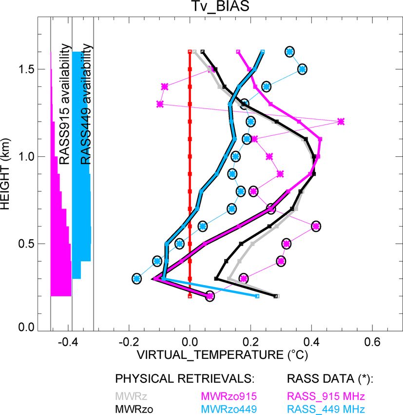
I. V. Djalalova et al.: Improving thermodynamic profile retrievals from microwave radiometers                                523

2     XPIA dataset                                               to ∼ 1 km a.g.l., and the transparent channels, 51–56 GHz,
                                                                 that are more informative above 1 km a.g.l. Both MWRs ob-
The data used in our analysis were collected during the XPIA     served at the zenith and at 15 and 165◦ elevation angles in
experiment, held in spring 2015 (March–May) at NOAA’s            the north–south plane (referred to as oblique elevation scans
BAO site, in Erie, Colorado (40.0451◦ N, 105.0057◦ W, ele-       and used as their average hereafter; note zenith views have
vation 1584 m.s.l.). XPIA was the last experiment conducted      a 90◦ elevation angle). However, when MWRs are deployed
at this facility, as after almost 40 years of operations the     in locations with unobstructed views, oblique scans can be
BAO 300 m tower was demolished at the end of 2016 (Wolfe         performed down to 5◦ elevation angles and may provide bet-
and Lataitis, 2018). XPIA was designed to assess the capa-       ter temperature profile accuracy in the lowest 0–1 or even
bility of different remote sensing instruments for quantify-     0–2 km a.g.l. layers (Crewell and Löhnert, 2007).
ing boundary layer structure and was a preliminary study as         In addition, each MWR was provided with a separate sur-
many of these same instruments were later deployed, among        face sensor to measure pressure, temperature, and relative hu-
other campaigns, for the second Wind Forecast Improvement        midity at the installation level that was ∼ 2.5 m a.g.l.. Verti-
Project WFIP2 (Shaw et al., 2019; Wilczak et al., 2019),         cal profiles of temperature (T ), water vapor density (WVD),
which investigated flows in complex terrain for wind en-         and relative humidity (RH) were retrieved in real time during
ergy applications, where they were for example used to study     XPIA every 2–3 min using a neural network (NN) approach
cold air pools (Adler et al., 2021) and gap flow character-      provided by the manufacturer of the radiometer (Solheim et
istics (Neiman et al., 2019; Banta et al., 2020). The list of    al., 1998a, b; Ware et al., 2003). Although the physical re-
the deployed instruments included active and passive remote-     trieval configurations used in this study do not exactly match
sensing devices and in situ instruments mounted on the BAO       the NN retrieval configurations, a comparison of both physi-
tower. Data collected during XPIA are publicly available         cal and neural network retrievals to the radiosonde tempera-
at https://a2e.energy.gov/projects/xpia (last access: 20 Jan-    ture data is presented in Appendix A.
uary 2022). A detailed description of the XPIA experiment           Both MWRs nominally operated from 9 March to
can be found in Lundquist et al. (2017), while a specific look   7 May 2015, although the MWR-NOAA was unavailable
at the accuracy of the instruments used in this study can be     between 5–27 April 2015. For the overlapping dates, tem-
found in Bianco et al. (2017).                                   perature profiles retrieved from the two MWRs showed very
                                                                 good agreement with less than 0.5 ◦ C bias and 0.994 corre-
2.1    MWR measurements                                          lation (Bianco et al., 2017). For this reason, and because the
                                                                 MWR-CU was available for a longer time period, only the
Two identical MWRs (Radiometrics MP-3000A) managed               MWR-CU (hereafter simply called MWR) is used.
by NOAA (MWR-NOAA) and by the University of Colorado
(MWR-CU) were deployed next to each other at the visi-           2.2   WPR–RASS measurements
tor center ∼ 600 m south of the BAO tower (see Lundquist
et al., 2017, for a detailed map of the study area). Prior to    Two NOAA wind profiling radars (WPRs), operating at fre-
the experiment, both MWRs were thoroughly serviced (sen-         quencies of 915 and 449 MHz, were deployed at the visitor
sor cleaning, radome replacement, etc.) and calibrated using     center (same location as the MWR) during XPIA. These sys-
an external liquid nitrogen target and an internal ambient       tems are primarily designed to measure the vertical profile
target. MWRs are passive devices which record the natural        of the horizontal wind vector, but co-located RASSs also en-
microwave emission in the water vapor and oxygen absorp-         able the observation of profiles of virtual temperature in the
tion bands from the atmosphere, providing measurements of        lower atmosphere, with different resolutions and height cov-
the brightness temperatures. Both MWRs have 35 channels          erage depending on the WPR. Thus, the RASS associated
spanning a range of frequencies, with 21 channels in the         with the 915 MHz WPR (hereafter referred to as RASS 915)
lower (22–30 GHz) K-band frequency band, of which 8 chan-        measured virtual temperature from 120 to 1618 m with a
nels were used during XPIA (22.234, 22.5, 23.034, 23.834,        vertical resolution of 62 m, and the 449 MHz RASS (here-
25, 26.234, 28, and 30 GHz) and 14 channels in the higher        after referred to as RASS 449) sampled the boundary layer
(51–59 GHz) V-band frequency band, all of which were used        from 217 to 2001 m with a vertical resolution of 105 m.
in XPIA (51.248, 51.76, 52.28, 52.804, 53.336, 53.848, 54.4,     The maximum height reached by the RASS is a function of
54.94, 55.5, 56.02, 56.66, 57.288, 57.964, and 58.8 GHz).        both radar frequency and atmospheric conditions (May and
Frequencies in the K-band are more sensitive to water vapor      Wilczak, 1993) and is usually lower for RASS 915 data, as
and cloud liquid water, while frequencies in the V-band are      will be shown later in the analysis.
sensitive to atmospheric temperature due to the absorption          The RASS data were processed using a radio frequency in-
of atmospheric oxygen (Cadeddu et al., 2013). V-band fre-        terference (RFI) removal algorithm (performed on the RASS
quencies or channels can also be divided into two categories:    spectra), a consensus algorithm (Strauch et al., 1984) per-
the opaque channels, 56.66 GHz and higher, that are more         formed on the moment data using a 60 % consensus thresh-
informative in the layer of the atmosphere from the surface      old, a Weber–Wuertz outlier removal algorithm (Weber et

https://doi.org/10.5194/amt-15-521-2022                                              Atmos. Meas. Tech., 15, 521–537, 2022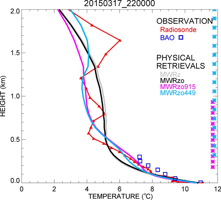
524                       I. V. Djalalova et al.: Improving thermodynamic profile retrievals from microwave radiometers

al., 1993) performed on the consensus averages, and a RASS         tistical evaluation. These restrictions lowered the number of
range-correction algorithm (Görsdorf and Lehmann, 2000)            total radiosonde launches used in this study to 52.
using an average relative humidity setting of 50 % deter-
mined from the available observations.
                                                                   3     Physical retrievals
2.3   BAO data
                                                                   One way to combine the active and passive instruments
The BAO 300 m tower was built in 1977 to study the plan-           would be to use the RASS observations up to their maximum
etary boundary layer (Kaimal and Gaynor, 1983). During             available height and stitch them with the profiles obtained
XPIA, measurements were collected at the surface (2 m) and         from a physical iterative method using MWR data. To do
at six higher levels (50, 100, 150, 200, 250, and 300 m a.g.l.).   this, the moisture contribution to the RASS virtual tempera-
Each tower level was equipped with two sonic anemometers           tures could be removed by using either the relative humidity
on orthogonal booms and one sensor based on a Sensiron             measured by the MWR or by a climatology of the moisture
SHT75 solid-state sensor to measure temperature and rela-          term. However, merging these different profiles could result
tive humidity with a time resolution of 1 s, and averaged over     in artificial jumps at the connecting heights.
5 min. The more accurate temperature and water vapor obser-           Alternatively, a physical retrieval (PR) iterative approach
vations (Horst et al., 2016) at the BAO tower 2 m a.g.l. level     can be used to retrieve vertical profiles of thermodynamic
are used in the physical retrieval in place of the less accurate   properties from the MWR and RASS observations in a syn-
MWR surface sensor.                                                ergistic manner (e.g., Maahn et al., 2020; Turner and Löhn-
                                                                   ert, 2021). In this case, an optimal estimation-based physical
                                                                   retrieval is initialized with a climatologically reasonable pro-
2.4   Radiosonde measurements                                      file of temperature and water vapor and is iteratively repeated
                                                                   until the computed brightness temperatures match those ob-
Between 9 March and 7 May 2015, while the MWR was op-              served by the MWR within the uncertainty of the observed
erational, radiosondes were launched by the National Center        brightness temperatures and the RASS virtual temperatures
for Atmospheric Research (NCAR) assisted by several stu-           within their uncertainties (Rodgers, 2000; Turner and Löhn-
dents from the University of Colorado over three selected          ert, 2014; Cimini et al., 2018; Maahn et al., 2020).
periods, one each in March, April, and May. All radiosondes
were Vaisala model RS92. There were a total of 59 launches,        3.1    Iterative retrieval technique
mostly four times per day, around 14:00, 18:00, 22:00, and
02:00 UTC (08:00, 12:00, 16:00, and 20:00 local standard           For this study, the PR uses the TROPoe retrieval algorithm
time, LST). The first 35 launches, between 9–19 March, were        (formerly AERIoe; Turner and Löhnert, 2014; Turner and
done from the visitor center, while 11 launches between 15–        Blumberg, 2019; Turner and Löhnert, 2021). This algorithm
22 April, and 13 launches between 1–4 May were done from           is able to use radiance data from microwave radiometers, in-
the water tank site, ∼ 1000 m away from the visitor center         frared spectrometers, and other observations as input. The
(see Lundquist et al., 2017, for a detailed map of the study       microwave radiative transfer model, MonoRTM (Clough et
area). The radiosonde measurements included temperature,           al., 2005), serves as the forward model, which is fully func-
dew point temperature, and relative humidity to altitudes usu-     tional for the microwave region and was intensively evalu-
ally higher than 10 km a.g.l., with measurements every few         ated previously on MWR measurements (Payne et al., 2008;
seconds. As a first step, for additional verification, the ra-     2011).
diosonde data from the 59 launches taken between 9 March              We start with the state vector Xa = [T , Q, LWP]T , where
and 4 May 2015 were compared to the BAO tower mea-                 superscript T denotes transpose, and vectors and matrices are
surements, up to 300 m a.g.l.. These observed datasets match       shown in bold. T (K) and Q (g kg−1 ) are temperature and
very well, with a correlation coefficient of 0.99 and a stan-      water vapor mixing ratio profiles at 55 vertical levels from
dard deviation of ∼ 0.7 ◦ C. However, one radiosonde pro-          the surface up to 17 km, with the distance between the levels
file showed a large bias (>5 ◦ C) against all seven levels of      increasing geometrically with height. LWP is the liquid water
BAO temperature measurements and all available T v mea-            path in g m−2 that measures the integrated content of liquid
surements from the RASS 915 (eight measurements up to              water in the entire vertical column above the MWR and is
600 m a.g.l.) and from the RASS 449 (nine measurements up          a scalar. For this study, X a has dimensions equal to 111 × 1
to 1100 m a.g.l.); therefore this particular radiosonde profile    (two vectors T and Q with 55 levels each, and LWP). The
was excluded from the statistical analysis. Moreover, while        retrieval framework of Turner and Blumberg (2019) is used,
accurate RASS data can be collected during rain, MWR data          but only using MWR data (no spectral infrared). Here, we
could be potentially deteriorated due to water deposition on       demonstrate the extension of the retrieval to include RASS
the radome. Therefore, six profiles (three for 13 March and        profiles of T v and the resulting impact this has on the re-
one each on 1, 3, and 4 May) were eliminated from the sta-         trieved temperature profiles and information content.

Atmos. Meas. Tech., 15, 521–537, 2022                                                 https://doi.org/10.5194/amt-15-521-2022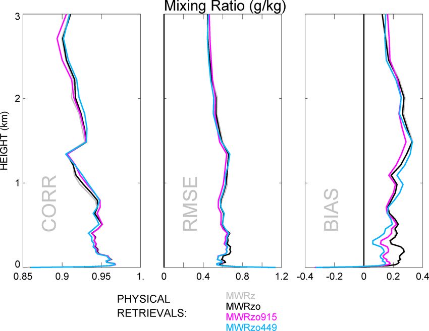
I. V. Djalalova et al.: Improving thermodynamic profile retrievals from microwave radiometers 525
The observation vector Y includes temperature and water Tsfc
Qsfc
vapor mixing ratio measured at the surface in situ and spec-
Y4 = T bzenith+oblique
tral T b measured by the MWR. The MonoRTM model F is
used as the forward model from the current state vector X T vRASS449
2
and is then compared to the observation vector Y , iterating
σTsfc 0 0 0
until the difference between F (X) and Y is small within a 0 2
σQsfc 0 0
specified uncertainty (Eq. 1). Sε4 =
0 0 σ 2T bzenith+oblique 0
Xn+1 = Xn + (S−1 T −1 −1 T −1
a + K Sε K) K Sε [Y − F (X n )
0 0 0 σ 2T vRASS449
+ K(X n − Xa )] (1) Note that the 2 m surface-level observations of temperature
and water vapor mixing ratio (Tsfc and Qsfc , respectively)
with are included as part of the observation vector Y , and thus the
uncertainties (0.5 K for temperature and less than 0.4 g kg−1
T
Xa = Q for mixing ratio) in these observations are included in Sε .
LWP The mean state vector of the climatological estimates, or a
“prior” vector X a , is a key component in the optimal estima-
σ2 σ 2T Q 0 tion framework, and it is the first guess of the state vector X,
2T T
Sa = σ QT σ 2QQ 0
X 1 , in Eq. (1). It provides a constraint on the ill-posed inver-
0 0 2
σLWP sion problem. The prior is calculated independently for each
∂ Fi month of the year from climatological sounding profiles (us-
Kij = , ing 10 years of data) in the Denver area. The covariance ma-
∂ Xj
trix, Sa , of the “prior” vector includes not only temperature
where i and j in the Kij definition mark channel and vertical or water vapor variances but also the covariances between
level, respectively. The superscripts T and −1 in Eq. (1) indi- them. Using around 3000 radiosondes launched by the NWS
cate the transpose and inverse matrices, respectively. The ob- in Denver, each radiosonde profile is interpolated to the ver-
servation vector Y and the covariance matrix of the observed tical levels used in the retrieval, after which the covariance of
data, Sε , depending on the configuration used, are equal to temperature and temperature, temperature and humidity, and
the following. humidity and humidity is computed for different levels. LWP
is arbitrarily assigned in Xa , with large values chosen for its
Tsfc uncertainty in Sa , so that it does not impact (constrain) the
Y 1 = Qsfc retrieval. Presently, the assumed uncertainty in LWP in the
T bzenith prior is assigned to 200 g m−2 in the TROPoe configuration
σT2sfc 0 0
file.
2 Four configurations are chosen for the observational vec-
Sε1 = 0 σQ 0
sfc
tor Y (Y 1 , Y 2 , Y 3 , and Y 4 ). In each of these, the surface
0 0 σ 2T bzenith observations are obtained by the 2 m BAO in situ measure-
ments of temperature and humidity. The MWR provides T b
measurements from 22 channels from the zenith scan for the
Tsfc
zenith-only configuration (Y 1 ), while when using the zenith
Y 2 = Qsfc
plus oblique T b inputs (Y 2 , Y 3 , and Y 4 ) the same 22 chan-
T bzenith+oblique
2 nels were used from the zenith scans together with only the
σTsfc 0 0 four opaque channels (56.66, 57.288, 57.964, and 58.8 GHz)
2
Sε2 = 0 σQ 0 from the oblique scans. Using additional measurements from
sfc
0 0 2
σ T bzenith+oblique the co-located radar systems with RASS, the observational
vector is further expanded with either RASS 915 (Y 3 ) or
RASS 449 (Y 4 ) virtual temperature observations. The co-
Tsfc variance matrix of the observed data, Sε , depends on the cho-
Qsfc sen Y i as seen in the matrix Sεi (with i = 1 : 4) descriptions,
Y3 = T bzenith+oblique
with increasing dimensions from Y 1 to Y 2 and additional
T vRASS915 increasing dimensions to Y 3 or Y 4 through the multi-level
2
σTsfc 0 0 0
measurements of the RASS (Turner and Blumberg, 2019).
0 2 Table 1 summarizes the observational information included
σQsfc 0 0
Sε3 =
in these four different configurations of the PR.
0 0 σ 2T bzenith+oblique 0
0 0 0 σ 2T vRASS915
https://doi.org/10.5194/amt-15-521-2022 Atmos. Meas. Tech., 15, 521–537, 2022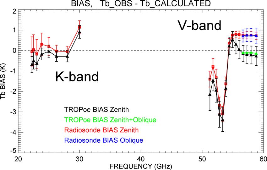
526                        I. V. Djalalova et al.: Improving thermodynamic profile retrievals from microwave radiometers

Table 1. Four PR configurations corresponding to the four observational Y i vectors in Eq. (1).

                                              Tsfc    Qsfc    T b zenith    T b oblique   T v RASS915   T v RASS449
                        Y 1 = MWRz            ×       ×       ×
                        Y 2 = MWRzo           ×       ×       ×             ×
                        Y 3 = MWRzo915        ×       ×       ×             ×             ×
                        Y 4 = MWRzo449        ×       ×       ×             ×                           ×

   The uncertainty in the MWR T b observations was set to                     For both approaches, the first step is to identify clear-sky
the standard deviation from a detrended time-series analy-                 periods during which the bias can be estimated (to elimi-
sis for each channel during cloud-free periods. The method                 nate uncertainties associated with clouds), and subsequently
to detect those cloud-free periods is described in detail in               the bias can be removed from the observed MWR T b s. One
Sect. 3.2. The derived uncertainties ranged from 0.3 to 0.4 K              method to identify clear-sky times is to use a time series of
in the 22 to 30 GHz channels and 0.4 to 0.8 K in the 52 to                 T b observations in the 30 GHz liquid-water-sensitive chan-
60 GHz channels. We assumed that there was no correlated                   nel of the MWR.
error between the different MWR channels.                                     The standard deviation of the MWR T b in the 30 GHz
   For the RASS, co-located RASS and radiosonde profiles                   channel is calculated over a time frame of 1 h centered at the
were compared, and the standard deviation of the differences               radiosonde launch time. The data from the zenith scan and
in T v was determined as a function of the radar’s signal-to-              the averaged oblique scans are reviewed separately. Liquid-
noise ratio (SNR). This relationship resulted in uncertainties             cloud-free periods were identified by cases where the tem-
that ranged from 0.8 at high SNR values to 1.5 K at low SNR                poral standard deviation was small (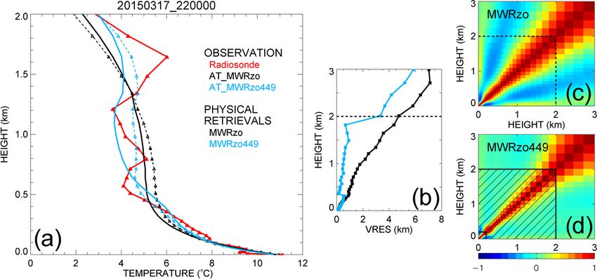
I. V. Djalalova et al.: Improving thermodynamic profile retrievals from microwave radiometers                                   527

                                                                    or that the sensitivity to the scene (e.g., zenith or off-zenith)
                                                                    is small.
                                                                       The bias-correction methods were applied by removing
                                                                    the corresponding calculated biases from the MWR T b ob-
                                                                    servations before the retrievals were performed. Later in
                                                                    Sect. 4, differences in the retrieved temperature profiles will
                                                                    be shown when using the two bias-correction approaches.
                                                                    These differences will be more evident in the temperature
                                                                    profiles exhibiting near-ground temperature inversions.
                                                                       However, the final goal of this study is not to assess the
                                                                    sensitivity to different bias-correction approaches but to ver-
                                                                    ify that the inclusion of RASS observations does improve
                                                                    retrieved temperature profiles, independently of the bias-
                                                                    correction method used.
Figure 1. T b biases derived from the radiosonde BC method (and
TROPoe BC method) in all 22 MWR channels of the zenith scan in
red (and in black) and in the four opaque channels of the oblique   3.3   Analysis of physical retrieval characteristics
scans in blue (and in green).

                                                                    The retrieved profiles of the four different PR configura-
                                                                    tions presented in Table 1 (MWRz, MWRzo, MWRzo915,
retrieved profiles (Y 1 ) of those selected clear-sky days. This    MWRzo449) were compared to the radiosonde profiles. To
method identified spectral calibration errors in the MWR ob-        compare radiosonde observations against the PR profiles, all
servations that could not be explained by physically realistic      radiosonde profiles were interpolated vertically to the same
atmospheric profiles. This bias-correction technique, which         PR heights, and PR profiles were averaged in the time win-
accounts for those unphysical spectral calibration features,        dow between 15 min before and 15 min after each radiosonde
will be referred to as “TROPoe BC”.                                 launch. Since the radiosonde ascends quite quickly in the
   Figure 1 shows the T b biases found for all 22 MWR chan-         lowest kilometers of the atmosphere (∼ 15–20 min to reach
nels from both bias-correction approaches. The biases calcu-        5 km), the 30 min temporal window is estimated to be rep-
lated with the radiosonde BC scheme are shown for all chan-         resentative of the same volume of the atmosphere measured
nels used in our analysis: 22 channels of the zenith scan, in       by the radiosonde. BAO tower temperature and mixing ratio
red, and four V-band opaque channels of the oblique scans,          data at the seven available levels were used as an additional
in blue. The black and green triangles represent the biases         validation dataset, without any vertical interpolation, aver-
calculated using the TROPoe BC approach for zenith and              aged in the time window between 15 min before and 15 min
for zenith+oblique scans, respectively. All biases are pre-         after each radiosonde launch.
sented with associated uncertainties (error bars representing          As an example of the different temperature retrievals and
the standard deviation over all radiosondes for radiosonde          their relative performance, data obtained on 17 March 2015
BC and mean observation T b vector uncertainties for 4 cho-         at 22:00 UTC are presented in Fig. 2. Temperature profiles
sen clear-sky days for TROPoe BC).                                  up to 2 km a.g.l. retrieved from the four PR configurations
   The biases from the two bias-correction schemes are              (MWRz, MWRzo, MWRzo915, MWRzo449, using the ra-
within the uncertainties of each other for most of the chan-        diosonde BC) are compared to the radiosonde data in red
nels except at the higher frequencies in the V-band. Biases         and to the BAO measurements in blue squares. Note that
in the most opaque channels are significantly affected by the       all four of the PRs match the BAO observations reason-
accuracy of the boundary layer temperature profiles. When           ably well near the ground. The MWRz and MWRzo pro-
TROPoe BC is used, a monthly average prior temperature              files are very smooth and depart quite substantially from the
profile is used in the PR and thus differences between this         radiosonde measurements and are unable to reproduce the
prior profile and the actual temperature profile can result in      more detailed structure of the atmospheric temperature pro-
a spectral bias in the more opaque MWR channels. On the             file measured by the radiosonde, while the MWRzo449 pro-
contrary, the radiosonde BC uses a direct measurement of the        file (in light blue) demonstrates a better agreement with both
temperature profile (from the radiosonde), and thus is more         the radiosonde and BAO measurements (blue squares). The
accurate. It is also important to note that, in both approaches,    MWRzo915 profile (in magenta) also tries to follow the ele-
the biases in the opaque channels for zenith and for oblique        vated temperature inversion observed by the radiosonde, suc-
scans (for radiosonde BC these are red and blue, respectively,      cessful only in the lower part of the atmosphere (below 1 km
and for the TROPoe BC these are black and green, respec-            a.g.l.) where RASS 915 measurements are available. This be-
tively) are very similar to each other. This supports the as-       havior will also be addressed in the following section and in
sumption that the true bias is nearly independent of the scene,     the statistical analysis presented later in the paper.

https://doi.org/10.5194/amt-15-521-2022                                                  Atmos. Meas. Tech., 15, 521–537, 2022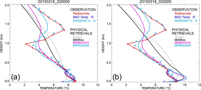
528                       I. V. Djalalova et al.: Improving thermodynamic profile retrievals from microwave radiometers

                                                                    the various retrievals and the radiosonde profiles due to very
                                                                    different vertical resolutions of these profiles (Turner and
                                                                    Löhnert, 2014).
                                                                       Smoothed radiosonde observed profiles can be computed
                                                                    using the averaging kernel as
                                                                    X smoothedradiosonde = Akernel(Xradiosonde − Xa ) + Xa .     (4)
                                                                    The Akernel in Eq. (2) depends on the retrieval parameters
                                                                    (e.g., which datasets are used in the Y vector, the values as-
                                                                    sumed in the observation covariance matrix Sε , and the sen-
                                                                    sitivity of the forward model), so for our four PR configu-
                                                                    rations it is possible to calculate four different kernels from
                                                                    Eq. (2).
                                                                       For each of the four Akernels, a smoothed radiosonde
                                                                    profile can be computed for each radiosonde profile using
                                                                    Eq. (4). In the presence of temperature inversions or other
                                                                    particular structures in the atmosphere, these smoothed pro-
                                                                    files can be quite different from each other and also from
                                                                    the original unsmoothed radiosonde profile. Consequently,
Figure 2. Temperature profiles obtained by the four PR configura-   while comparison of the retrievals to the relative Akernel-
tions, after applying the radiosonde BC to the MWR T b s: MWRz in   smoothed radiosonde profiles can be used to minimize the
gray, MWRzo in black, MWRzo915 in magenta, and MWRzo449             vertical representativeness effects due to the different vertical
in light blue. These retrievals are compared to radiosonde mea-
                                                                    resolutions of these profiles, we note that a statistical com-
surements, in red, and BAO tower observations, as blue squares.
The heights with available RASS virtual temperature measurements
                                                                    parison between the four configurations of the observational
(RASS 915 in magenta and RASS 449 in light blue) are marked by      vector would not be fair if each of their retrieved profiles
the asterisks on the right y axis.                                  is compared to a different Akernel-smoothed radiosonde
                                                                    profile. Therefore, in the statistical analysis presented later
                                                                    in the paper (Sect. 4.2), mean bias, root-mean-square error
   An asset of TROPoe is that several characteristics of            (RMSE), and Pearson correlation coefficients will be com-
the PRs can be obtained from two matrices, the averaging            puted between the various TROPoe retrieval configurations
kernel, Akernel, and the posterior covariance matrix, Sop           and the unsmoothed radiosonde profiles, just interpolated to
(Masiello et al., 2012; Turner and Löhnert, 2014, Turner and        the same vertical levels of the retrieved profiles.
Bloomberg, 2019), calculated as                                        The ATkernel can help understand the differences in the
                                                                    retrieved temperature profiles obtained by the configura-
Akernel = B−1 KT S−1
                  ε K                                        (2)    tions using additional RASS data, shown in the example of
                                                                    Fig. 2. Figure 3a includes the temperature profiles of the ra-
and                                                                 diosonde (unsmoothed and ATkernel’s smoothed) and PRs
                                                                    of MWRzo and MWRzo449 for the same example as in
Sop = B−1 ,                                                  (3)
                                                                    Fig. 2. Due to the inclusion of RASS measurements, the
where                                                               ATkernel-smoothed radiosonde profile of the MWRzo449
                                                                    configuration (dashed light blue line) is closer to the original
          T −1
B = S−1
     a + K Sε K.
                                                                    radiosonde data (in red) compared to the black dashed pro-
                                                                    file of the MWRzo’s ATkernel-smoothed radiosonde profile.
All matrices, Akernel, Sop , and B, have dimensions 111 ×           Additionally, the rows of the ATkernel provide a measure
111 in our configuration. While the top left corner of the          of the retrieval smoothing as a function of altitude, so the
Akernel matrix (1 : 55, 1 : 55) is devoted to temperature,          full width at half maximum (FWHM) of each ATkernel row
called ATkernel in the text, the next (56 : 110, 56 : 110) el-      estimates the vertical resolution of the retrieved solution at
ements are devoted to the water vapor mixing ratio, called          each vertical level (Maddy and Barnet, 2008; Merrelli and
AQKernel.                                                           Turner, 2012). Plots of this vertical resolution as a function
   The Akernel provides useful information about the cal-           of the height for the MWRzo PR and for the MWRzo449 PR
culated retrievals, such as vertical resolution and degrees of      are included in Fig. 3b. This plot shows that the additional
freedom for signal at each level. The rows of the Akernel           observations from the RASS 449 significantly improve the
provide the smoothing functions (Rodgers, 2000) that could          vertical resolution of the retrievals.
be applied to the radiosonde profiles (Eq. 4) to minimize the          The posterior covariance matrix, Sop , provides a measure
vertical representativeness error in the comparison between         of the uncertainty of the retrievals while the square root of

Atmos. Meas. Tech., 15, 521–537, 2022                                                  https://doi.org/10.5194/amt-15-521-2022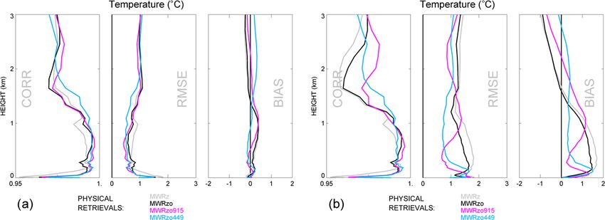
I. V. Djalalova et al.: Improving thermodynamic profile retrievals from microwave radiometers                                    529

Figure 3. (a) Observed temperature profiles from radiosonde in red, from ATkernel-smoothed radiosonde, AT_MWRzo in dashed black,
and AT_MWRzo449 in dashed light blue; PRs from MWRzo PR in solid black, and from MWRzo449 PR in solid light blue. (b) Vertical
resolution (VRES) as a function of the height for the MWRzo PR (black) and for the MWRzo449 PR (light blue). (c, d) 3 × 3 km (37 ×
37 levels) Sop matrices, converted to correlation matrices, for the MWRzo PR (c) and for the MWRzo449 PR (d). Dashed lines on plots
(b–d) mark 2 km a.g.l. Hatched area on panel (d) marks the RASS measurement heights.

the diagonal of this matrix is used to specify the 1σ errors in     used for each retrieval height, computed as the full width at
the profiles of temperature or mixing ratio. Also, Sop shows        half maximum value of the averaging kernel. The cumula-
the level-to-level dependency of the retrievals and in an ideal     tive DFS profile (Fig. 4g) is a measure of the number of in-
case should have all non-diagonal elements equal to zero.           dependent pieces of information in the observations below
Converted to a correlation matrix, it is possible to visualize      the specified height. For example, at the 1 km a.g.l. level the
these dependencies, as presented in Fig. 3c, d. The use of          vertical resolution of MWRzo449 is 0.5 km (i.e., informa-
additional RASS data (MWRzo449 Sop , Fig. 3d) reduces the           tion from ±0.5 km around the retrieval height is considered
off-diagonal covariances, therefore substantially decreasing        in the retrieval), while all other retrievals use the information
the correlations in those areas compared to the MWRzo Sop           from more than ±1.5 km. Also, the DFS, as a cumulative
(Fig. 3c).                                                          measure, shows an increase in pieces of information from
   To understand the level-to-level correlations among the          MWRz to MWRzo for the whole profile and from MWRzo
four different retrieval configurations in Table 1, the Sop ma-     to MWRzo915 and to MWRzo449 above ∼ 0.2 km where
trices were averaged over all radiosonde events and converted       RASS data are available. The DFS of MWRzo915 is higher
to correlation matrices (Fig. 4). A clearly visible narrowing       compared to the DFS of MWRzo449 in the 0.2–0.5 km a.g.l.
of the spread around the main diagonal and correlation re-          layer because RASS 915 data have denser measurements
duction in the off-diagonal elements results by adding ad-          there. It is also important to note that there is no additional
ditional observations, from MWR zenith only (Fig. 4a), to           information added to any of the retrievals above 2 km a.g.l.;
MWR zenith-oblique (Fig. 4b), to the larger impact obtained         i.e., the slope of the cumulative DFS profiles are equal. De-
by the usage of the RASS 915 (Fig. 4c), concluding with the         spite that, the statistical analysis of the PRs up to 3 km a.g.l.,
RASS 449 (Fig. 4d) data. The mean retrieval uncertainty pro-        shown in Sect. 4, will prove that the retrieval improvements
file for each of the PR configurations is presented in Fig. 4e.     obtained by including the RASS are found even above the
The uncertainty of the MWRzo449 retrieval up to 1 km a.g.l.         height of the RASS measurement availability.
is around 0.5 ◦ C while the other retrievals have higher uncer-        The improvements from MWRz (in gray) to MWRzo
tainties of up to 1 ◦ C. The higher accuracy of the MWRzo449        (in black), to MWRzo915 (in magenta), and finally to
retrievals is because that configuration has more observa-          MWRzo449 (in light blue) are visible in all three panels
tional information compared to the other retrieval configu-         (Fig. 4e–g), whereas MWRzo449 has the lowest 1σ uncer-
rations.                                                            tainty and highest DFS compared to the other PRs, particu-
   Other statistically important features to analyze in the PRs,    larly below 2 km a.g.l., where RASS 449 measurements are
besides their uncertainty, are the vertical resolution already      available. Finally, it is interesting that below 200 m a.g.l. the
introduced in the example of Fig. 3b and the degree of free-        MWRzo915 has slightly smaller lowest 1σ uncertainty and
dom for signal (DFS). These two features, derived from the          vertical resolution relative to the MWRzo449, as could be
Akernels of each PR configuration, averaged over all ra-            expected due to the first available height of the RASS 915
diosonde events, are shown in Fig. 4f and g. The vertical           being lower (120 m a.g.l.) than the first available height for
resolution (Fig. 4f) shows the width of the atmosphere layer        the RASS 449 (217 m a.g.l.) and due to the finer vertical res-

https://doi.org/10.5194/amt-15-521-2022                                                  Atmos. Meas. Tech., 15, 521–537, 2022
530                       I. V. Djalalova et al.: Improving thermodynamic profile retrievals from microwave radiometers

Figure 4. (a–d) The mean Sop s, displayed as correlation matrices, for (a) MWRz, (b) MWRzo, (c) MWRzo915, and (d) MWRzo449,
averaged over all radiosonde events. The hatched area in panels (c) and (d) marks the RASS maximum measurement heights. (e) One-sigma
uncertainty derived from the posterior covariance matrix in ◦ C, (f) vertical resolution (VRES) in kilometers, and (g) cumulative degree
of freedom (DFS) as a function of height for temperature, averaged over all radiosonde events (MWRz is in gray, MWRzo is in black,
MWRzo915 is in magenta, and MWRzo449 is in light blue). Dashed lines mark 2 km a.g.l. in all panels.

olution of the 915 MHz RASS. This suggests that, if addi-             file closer to the radiosonde temperature profile than when
tional observations were available in the lowest several hun-         using TROPoe BC, for which the inversion in the tempera-
dred meters of the atmosphere where RASS measurements                 ture profile close to the surface is too accentuated (particu-
are not available, improvements might be even better closer           larly the black, magenta, and cyan lines, all of which used
to the surface, where temperature inversions, if present, are         oblique scan data).
sometimes difficult to retrieve correctly.                               The relative statistical behavior (Pearson correlation,
                                                                      RMSE, and bias) of the PRs for both temperature and mix-
                                                                      ing ratio against radiosondes is shown in Fig. 6, using both
4     Results                                                         bias-correction approaches. PRs obtained after applying the
                                                                      radiosonde BC (Fig. 6a) present overall smaller RMSE and
4.1    Statistical analysis of physical retrievals up to 3 km         bias (the latter almost equal to zero up to 3 km a.g.l.) and
       a.g.l.                                                         slightly higher correlations compared to the statistics of the
                                                                      PRs obtained after applying the TROPoe BC (Fig. 6b). This
Several cases were found during XPIA when the temperature             could be expected since for the comparison in Fig. 6a a
profile exhibited inversions, with the lowest happening in the        subset of the radiosondes was already used for the T b bias
surface layer. Figure 5 shows one of the most complex cases,          correction. Also, the different retrievals show a narrower
with several temperature inversions visible in the tempera-           distribution for the panels in Fig. 6a. Nevertheless, the re-
ture profile from the radiosonde (red line), in the temperature       sults obtained when applying either bias-correction meth-
measurements from the BAO tower (blue squares), and in the            ods (in Fig. 6a, b) consistently show the improvement ob-
virtual temperature measured by the RASS 449 (light blue              tained when the RASS observations are used, with relatively
triangles). Note that the virtual temperature profile is in close     smaller bias and RMSE in the 3 km layer a.g.l. The correla-
agreement with the temperature measured by radiosonde.                tion is mainly improved above 1 km, when RASS observa-
   Figure 5 also illustrates the difference in the temperature        tions are included.
profiles, especially between 0–300 m a.g.l., for the two dif-            Besides temperature profiles, the PRs also provide water
ferent bias-correction schemes, which show noticeable dif-            vapor mixing ratio profiles. It is understandable that the dif-
ferences in the biases of the opaque channels (especially im-         ferent configurations of PRs are not noticeably different from
portant for the near-ground retrievals) presented in Fig. 1. As       each other in relation to moisture, because the T v observa-
expected, the radiosonde BC method yielded a retrieved pro-

Atmos. Meas. Tech., 15, 521–537, 2022                                                    https://doi.org/10.5194/amt-15-521-2022
I. V. Djalalova et al.: Improving thermodynamic profile retrievals from microwave radiometers 531
Figure 5. As in Fig. 2 but for 18 March 2015 at 02:00 UTC. The RASS 449 virtual temperature is included as light blue triangles. Panels (a)
shows the PRs obtained after applying the radiosonde BC, and (b) shows the PRs obtained after applying the TROPoe BC on the MWR T b s.
Figure 6. Pearson correlation, RMSE, and mean bias for temperature profiles of MWRz in gray, MWRzo in black, MWRzo915 in magenta,
and MWRzo449 in light blue for the radiosonde BC bias-correction method in (a) and TROPoe BC method in (b).
tions from the RASS are dominated by the ambient temper-
ature (not moisture), and thus have little impact on the water
vapor retrievals. We found that the AQKernel values are al-
most identical for all four PR configurations (not shown). De-
tailed statistical evaluation of the PR mixing ratio profiles is
presented in Fig. 7, also averaged over all radiosonde events,
and shows very similar correlations, RMSEs, and biases for
all PRs, implying that the impact of including RASS obser-
vations in the retrieval is minimal on this variable. Finally, it
is noted that Fig. 7 shows the mixing ratio of the data from
TROPoe BC. The radiosonde BC mixing ratio results are al-
most identical.
4.2 Statistics for the profiles least close to the
climatology
Physical retrievals use climatological data as a constraint in Figure 7. Same as the panels in Fig. 6b, but for mixing ratio, when
the retrieval. Statistically, the averaged profiles of both tem- using the TROPoe BC method on the MWR T b s.
perature and moisture variables are very close to the climato-
logical averages. However, the most interesting and difficult
profiles to retrieve are the cases furthest from climatology
https://doi.org/10.5194/amt-15-521-2022 Atmos. Meas. Tech., 15, 521–537, 2022532 I. V. Djalalova et al.: Improving thermodynamic profile retrievals from microwave radiometers
(Löhnert and Maier, 2012). To check the behavior of the re- 4.3 Virtual temperature profile statistics
trieved data in such “extreme” cases, the RMSE was first cal-
culated for each radiosonde profile relative to the prior pro- Using the physical retrieval outputs, “retrieved virtual tem-
files for 37 vertical levels from the surface up to 3 km a.g.l., perature profiles” can also be calculated. In this section the
and then the 15 cases with the largest 0–3 km layer averaged direct comparison of these retrieved virtual temperature pro-
RMSEs compared to the prior were selected. files and RASS virtual temperature profiles to the original
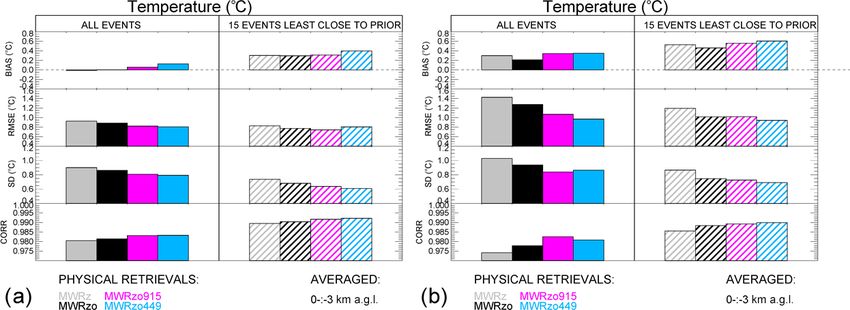
Figure 8 shows the temperature statistical analysis for the radiosonde is shown. With this comparison we want to show
entire radiosonde dataset (solid boxes) and for the 15 events how the biases of the retrieved profiles relate to the original
far from the climatological mean (hatched boxes) for bias, RASS T v biases.
RMSE, standard deviation of the differences between re- Figure 9 shows T v retrieved profile biases compared to the
trievals and radiosonde data, and Pearson correlation, calcu- original radiosonde data. These T v profiles and RASS 915
lated as the weighted averaged over the 37 vertical heights and RASS 449 T v bias data are interpolated onto a regular
up to 3 km a.g.l.1 . vertical grid, going from 200 m to 1.6 km with a 100 m reso-
Differences in the statistics when using the entire ra- lution, for easy comparison.
diosonde dataset or the 15 extreme profiles are noticeable While RASS 449 data are available at almost all heights
for all statistical estimators. The PRs that include RASS ob- up to 1.6 km, the RASS 915 data availability decreases con-
servations show better performance compared to the strictly siderably with height, decreasing to 50 % availability around
MWR-only PR profiles (i.e., MWRz and MWRzo) for al- 800 m a.g.l.. The PRs that include RASS data, MWRzo915
most all statistical comparisons. This improvement is larger and MWRzo449 are also marked with additional black lines
for the PRs using the TROPoe BC (Fig. 8b) compared to at the heights with at least 50 % of relative RASS data avail-
the PRs using the radiosonde BC (Fig. 8a). Three statisti- ability. In agreement with Fig. 6a, this figure clearly shows
cal estimators, RMSE, standard deviation, and Pearson cor- the superiority of the MWRzo449 and MWRzo915 (in the
relation, show overall better values for the 15 extreme cases layer with >50 % RASS data availability) compared to the
compared to the whole radiosonde dataset, for all PR con- MWRz and MWRzo configurations, which do not include
figurations and both BC approaches. This is due to the fact RASS data. For MWRzo449, RASS 449 data were almost
that for this dataset the monthly averaged radiosonde pro- always available; therefore it is easy to identify a similar-
files (for March and May particularly) depart quite substan- ity between the T v bias profiles of the RASS 449 and the
tially from the monthly prior profiles. For example, the aver- PRs including it. Thus, for the MWRzo449 the T v bias is
aged radiosonde profile in March is warmer by ∼ 7 ◦ C com- more uniform through the heights compared to all other PRs
pared to the March prior (and in May by ∼ 5 ◦ C) in the first that do not include RASS data. Moreover, it is noted that
3 km a.g.l.. Consequently, the extreme cases (mostly found in a roughly constant offset between the MWRzo449 T v and
March) have the warmest radiosonde temperature profiles but RASS 449 T v biases profiles, with their averaged difference
are overall closer to the monthly averaged radiosonde pro- equal to ∼ 0.08 ◦ C (when the radiosonde BC is used), and to
files. ∼ 0.32 ◦ C (when the TROPoe BC is used, not shown), over
Table 2 includes the same data as in Fig. 8 but as a percent- the ∼ 1.3 km (0.3–1.6 km) atmospheric layer where more
age of the improvement, compared to the MWRz retrievals. than 50 % of the RASS 449 measurements are available, uni-
The results presented in Table 2 show improvements in formly distributed through the heights. The inclusion of the
all statistical estimations when including RASS observa- RASS into the PRs does reduce the values of the biases in the
tions, with improvements in RMSE between 10 % and 20 %, retrievals even below the values of the RASS biases, because
demonstrating the positive impact derived by the inclusion of the combined information from RASS and MWR.
of the active measurements, regardless of the bias-correction
method used, but larger for the TROPoe BC data because
there is more room for improvement when this BC method 5 Conclusions
is used. Improvements in the Pearson correlation coefficients
are small because correlation, determined during XPIA by In this study, data collected during the XPIA field campaign
the overall temperature structure with height and diurnal cy- were used to test different configurations of a physical itera-
cle, is already good, leaving little room for improvement. tive retrieval (PR) approach in the determination of tempera-
ture and humidity profiles from data collected by microwave
radiometers, surface sensors, and RASS measurements. The
1 The vertical grid used in the PRs is not uniform, with more fre- accuracy of several PR configurations was tested: two con-
quent levels closer to the surface. If a simple average of the data figurations made use only of surface observations and MWR
from all levels is used, the near-surface layer will be weighted more observed brightness temperature (zenith only, MWRz; zenith
compared to the upper levels of the retrievals. To avoid this, a ver- plus oblique, MWRzo), while two others included the active
tical average over the lowest 3 km a.g.l. is performed using weights virtual temperature profile observations available from co-
at each vertical level determined by the distance between the levels. located RASS (one, RASS 915, associated with a 915 MHz
Atmos. Meas. Tech., 15, 521–537, 2022 https://doi.org/10.5194/amt-15-521-2022I. V. Djalalova et al.: Improving thermodynamic profile retrievals from microwave radiometers 533
Figure 8. From top to bottom: biases (retrievals minus radiosonde), RMSEs, standard deviations of the difference between retrievals and
radiosonde, and Pearson correlations for the four PR configurations, averaged from the surface to 3 km a.g.l., over all radiosonde data (solid
boxes), and over the 15 extreme cases (hatched boxes). The data in panel (a) use radiosonde BC and in (b) TROPoe BC on the MWR T b s.
Table 2. Retrieval improvements for different RASS/MWR configurations as a percentage compared to MWRz.
0–3 km a.g.l. All events 15 events least close to the prior
Radiosonde bias correction
MWRz MWRzo MWRzo MWRzo MWRz MWRzo MWRzo MWRzo
RASS915 RASS449 RASS915 RASS449
RMSE 0% 5% 11 % 13 % 0% 7% 10 % 3%
STTD 0% 4% 10 % 12 % 0% 8% 14 % 17 %
CORR 0% 0.1 % 0.3 % 0.3 % 0% 0.1 % 0.2 % 0.3 %
TROPoe bias correction
RMSE 0% 10 % 25 % 32 % 0% 15 % 15 % 21 %
STTD 0% 9% 18 % 16 % 0% 14 % 16 % 20 %
CORR 0% 0.4 % 0.9 % 0.7 % 0% 0.3 % 0.4 % 0.4 %
and the other, RASS 449, associated with a 449 MHz wind zenith scan. Of the PR configurations tested, generally better
profiling radar). Radiosonde launches were used for verifica- statistical agreement is found with the radiosonde observa-
tion of the retrieved profiles. In Appendix A, the performance tions when the RASS 449 is used together with the surface
of MWRz and MWRzo retrieved profiles and neural network observations and brightness temperature from the zenith and
retrieved profiles against the radiosondes was evaluated. averaged oblique MWR observations.
To remove any observational systematic error in the MWR The Akernel and the posterior covariance matrices for
T b observations, two bias-correction procedures were tested. temperature are used to derive the one-sigma uncertainty,
The first one takes advantage of the many radiosondes vertical resolution, and cumulative degree of freedom as a
launched during XPIA, and the second one uses profiles. function of height for the different PRs and the level-to-level
As expected, the radiosonde bias-correction method gives re- correlated uncertainty of the retrievals. Results show that the
trieved profiles closer to the radiosonde temperature profiles inclusion of the active instruments improves all of the above-
than when using the climatologically based method. Never- mentioned variables in the 0–3 km layer, including at heights
theless, our results show that regardless of the bias-correction between 2–3 km that are above the maximum RASS height.
method used, the inclusion of the observations from the ac- Thus, the positive impact of the RASS observations extends
tive RASS instruments in the PR approach improves the into the atmosphere above the height of measurements them-
accuracy of the temperature profiles by around 10 %–20 % selves.
compared to the PR configuration using only surface obser- Furthermore, 15 cases when temperature profiles from the
vations and MWR observed brightness temperature from the radiosonde observations were the furthest away from the
https://doi.org/10.5194/amt-15-521-2022 Atmos. Meas. Tech., 15, 521–537, 2022534 I. V. Djalalova et al.: Improving thermodynamic profile retrievals from microwave radiometers
Figure A1. Pearson correlation, RMSE, and mean bias for tem-
Figure 9. Bias of virtual temperature for all PR configurations com- perature profiles for MWRz in gray (and purple) and MWRzo in
pared to the original radiosonde measurements. A zero bias is de- black (and maroon) when the radiosonde BC (and the TROPoe BC)
noted by the red line. RASS data biases are marked by asterisks and method is applied. TROPoe temperature retrievals without any bias
by additional circles for the RASS data with more than 50 % avail- correction are shown for MWRz in dashed purple and for MWRzo
ability, according to the availability bar charts on the left. All PR in dashed maroon. Included in this figure are the NN temperature
profiles are derived after applying the radiosonde BC method. profiles, from the zenith scan (in beige) and from the averaged
oblique scans (in green).
mean climatological average were selected, and the statis-
tical comparison was reproduced over this subset of cases.
These are the cases usually the most difficult to retrieve and Appendix A
the most important to forecast; therefore, it is essential to im-
prove the retrievals in these situations. Even for this subset The neural network (NN) retrievals developed by the ven-
of selected cases the inclusion of active sensor observations dor explicitly for XPIA use a training dataset based on a
in the PRs is found to be beneficial. 5-year climatology of profiles from radiosondes launched at
Finally, the impact of the inclusion of RASS measure- the Denver International Airport, ∼ 56 km southeast from the
ments on the retrieved humidity profiles was considered, but XPIA site. NN-based MWR vertical retrieval profiles were
the inclusion of RASS observations did not produce signifi- obtained using the zenith or an average of two oblique ele-
cantly better results, compared to the configurations that do vation scans, 15 and 165◦ (not including the zenith), all with
not include them. This was not a surprise as RASS measures 58 levels extending from the surface up to 10 km, with a nom-
virtual temperature, effectively adding very little extra infor- inal vertical grid depending on the height (every 50 m from
mation to the water vapor retrieval. In this case a better op- the surface to 500 m, every 100 m from 500 m to 2 km, and
tion would be to consider adding other active remote sensors every 250 m from 2 to 10 km, a.g.l.).
such as water vapor differential absorption lidars (DIALs) to Figure A1 shows composite NN vertical profiles of tem-
the PRs. Turner and Löhnert (2021) showed that including perature (separately for the zenith and averaged obliques)
the partial profile of water vapor observed by the DIAL sub- calculated for radiosonde launch times and the correspond-
stantially increases the information content in the combined ing PR profiles already introduced in Fig. 6a, b with addi-
water vapor retrievals. Consequently, to improve both tem- tional TROPoe retrievals without any bias correction. For a
perature and humidity retrievals a synergy between MWR, proper comparison, only MWRz and MWRzo profiles are
RASS, and DIAL systems would likely be necessary. used, without including RASS measurements. It has to be
noted that since the “NN oblique” retrieval provided by the
manufacturer of the radiometer does not include the zenith,
this configuration cannot be considered exactly equivalent to
the MWRzo PR.
Atmos. Meas. Tech., 15, 521–537, 2022 https://doi.org/10.5194/amt-15-521-2022You can also read