Inductive Topic Variational Graph Auto-Encoder for Text Classification
←
→
Page content transcription
If your browser does not render page correctly, please read the page content below
Inductive Topic Variational Graph Auto-Encoder for Text Classification
                 Qianqian Xie                                          Jimin Huang
         Department of Computer Science,                        School of Computer Science,
            University of Manchester                                Wuhan University
      qianqian.xie@manchester.ac.uk                            huangjimin@whu.edu.cn

                    Pan Du                               Min Peng
  Department of Computer Science and Operations School of Computer Science,
         Research, University of Montreal           Wuhan University
         pandu@iro.umontreal.ca                   pengm@whu.edu.cn

                                        Jian-Yun Nie
                    Department of Computer Science and Operations Research,
                                    University of Montreal
                                  nie@iro.umontreal.ca

                     Abstract                           et al., 2019; Liu et al., 2020; Wang et al., 2020).
                                                        In addition to the local information captured by
    Graph convolutional networks (GCNs) have
    been applied recently to text classification and
                                                        CNN or RNN, GCNs learn word and document
    produced an excellent performance. However,         representations by taking into account the global
    existing GCN-based methods do not assume            correlation information embedded in the corpus-
    an explicit latent semantic structure of doc-       level graph, where words and documents are nodes
    uments, making learned representations less         connected by indexing or citation relations.
    effective and difficult to interpret. They are         However, the hidden semantic structures, such
    also transductive in nature, thus cannot han-
                                                        as latent topics in documents (Blei et al., 2003; Yan
    dle out-of-graph documents. To address these
    issues, we propose a novel model named in-          et al., 2013; Peng et al., 2018b), is still ignored by
    ductive Topic Variational Graph Auto-Encoder        most of these methods (Yao et al., 2019; Huang
    (T-VGAE), which incorporates a topic model          et al., 2019; Liu et al., 2020; Zhang et al., 2020),
    into variational graph-auto-encoder (VGAE)          which can improve the text representation and pro-
    to capture the hidden semantic information be-      vide extra interpretability (in which the proba-
    tween documents and words. T-VGAE inher-            bilistic generative process and topics make more
    its the interpretability of the topic model and
                                                        sense to humans compared to neural networks, i.e.
    the efficient information propagation mecha-
    nism of VGAE. It learns probabilistic repre-        topics can be visually represented by top-10 or 20
    sentations of words and documents by jointly        most probable word clusters). Although few stud-
    encoding and reconstructing the global word-        ies such as (Wang et al., 2020) have proposed incor-
    level graph and bipartite graphs of documents,      porating a topic structure into GCNs, the topics are
    where each document is considered individ-          extracted in advance from the set of documents, in-
    ually and decoupled from the global corre-          dependently from the graph and information prop-
    lation graph so as to enable inductive learn-       agation among documents and words. We believe
    ing. Our experiments on several benchmark
                                                        that the topics should be determined in accordance
    datasets show that our method outperforms the
    existing competitive models on supervised and       with   the connections in the graph. For example,
    semi-supervised text classification, as well as     the fact that two words are connected provides ex-
    unsupervised text representation learning. In       tra information that these words are on a similar
    addition, it has higher interpretability and is     topic(s). Moreover, existing GCN-based methods
    able to deal with unseen documents.                 are limited by their transductive learning nature, i.e.
                                                        a document can be classified only if it is already
1 Introduction
                                                        seen in the training phase (Wang et al., 2020; Yao
Recently,       graph convolutional networks            et al., 2019; Liu et al., 2020). The lack of inductive
(GCNs)(Kipf and Welling, 2017; Veličković             learning ability for unseen documents is a critical
et al., 2018) have been successfully applied to         issue in practical text classification applications,
text classification tasks (Peng et al., 2018a; Yao      where we have to deal with new documents. It is
                                                     4218
                        Proceedings of the 2021 Conference of the North American Chapter of the
              Association for Computational Linguistics: Human Language Technologies, pages 4218–4227
                           June 6–11, 2021. ©2021 Association for Computational Linguistics
Table 1: Comparison with related work. We compare ational Bayes (AEVB) method to make effi-
the manner of model learning, whether incorporate the cient black-box inference of our model.
latent topic structure and the manner of topic learning
of these models.
3. Experimental results on benchmark datasets
Model Explainability Learning Topics demonstrate that our method outperforms the
TextGCN (Yao et al., 2019) - transductive - existing competitive GCN-based methods on
TensorGCN (Liu et al., 2020) - transductive -
DHTG (Wang et al., 2020)
p
transductive static supervised and semi-supervised text classifi-
T-GCN (Huang et al., 2019) - inductive -
TG-Trans (Zhang and Zhang, 2020) - inductive -
cation tasks. It also outperforms topic models
TextING (Zhang et al., 2020) - inductive - on unsupervised text representation learning.
HyperGAT (Ding et al., 2020) -
p inductive -
Our model inductive dynamic
2 Related Work
intuitive to decouple documents with the global 2.1 Graph based Text Classification
graph and treat each document as an independent
graph (Huang et al., 2019; Zhang et al., 2020; Ding Recently, GCNs have been applied to various NLP
et al., 2020; Zhang and Zhang, 2020; Xie et al., tasks (Zhang et al., 2018; Vashishth et al., 2019).
2021). However, no attempt has been made to ad- For example, TextGCN (Yao et al., 2019) was pro-
dress both aforementioned issues. posed for text classification, which enriches the
To address these issues, we incorporate the topiccorpus-level graph with the global semantic infor-
model into variational graph auto-encoder (VGAE), mation to learn word and document embeddings.
and propose a novel framework named inductive Inspired by it, Liu et al. (Liu et al., 2020) fur-
Topic Variational Graph Auto-Encoder (T-VGAE). ther considered syntactic and sequential contextual
T-VGAE first learns to represent the words in a information and proposed TensorGCN. However,
latent topic space by embedding and reconstructing none of them utilized the latent semantic structures
the word correlation graph with the GCN proba- in the documents to enhance text classification. To
bilistic encoder and probabilistic decoder. Take address the issue, (Wang et al., 2020) proposed
the learned word representations as input, a GCN- dynamic HTG (DHTG), in an attempt to integrate
based message passing probabilistic encoder is the topic model into graph construction. DHTG
adopted to generate document representations via learned latent topics from the document-word cor-
information propagation between words and doc- relation information (similar to traditional topic
uments in the bipartite graph. We compare our models), which will be used for GCN based doc-
model with existing related work in Table 1. Dif- ument embedding. However, the topics in DHTG
ferent from previous approaches, our method uni- were learned independently from the word relation
fies topic mining and graph embedding learning graph and the information propagation process in
with VGAE, thus can fully embed the relations be- the graph, in which word relations are ignored.
tween documents and words into dynamic topics Moreover, the existing GCN-based methods also
and provide interpretable topic structures into repre-
require a pre-defined graph with all the documents
sentations. Besides, our model builds a document- and cannot handle out-of-graph documents, thus
independent word correlation graph and a word- limiting their practical applicability.
document bipartite graph for each document in- To deal with the inductive learning problem,
stead of a corpus-level graph to enable inductive (Huang et al., 2019; Zhang et al., 2020; Ding et al.,
learning. 2020; Zhang and Zhang, 2020) proposed to con-
The main contributions of our work are as fol- sider each document as an independent graph for
lows: text classification. However, the latent semantic
1. We propose a novel model T-VGAE based on structure and interpretability are still ignored in
topic models and VGAE, which incorporates these methods. Different from previous approaches,
latent topic structures for inductively docu- we aim to deal with both issues of dynamic topic
ment and word representation learning. This structure and inductive learning. We propose to
makes the model more effective and inter- combine the topic model and graph based infor-
pretable. mation propagation in a unified framework with
VGAE to learn interpretable representations for
2. we propose to utilize the auto-encoding vari- words and documents.
42192.2 Graph Enhanced Topic Models words in document t and v is the vocabulary of size
V.
There are also studies trying to enhance topic mod-
From the whole corpus, we build a word cor-
els with efficient message passing in the graph data
relation graph G = (v, e) containing word nodes
structure of GCNs. GraphBTM (Zhu et al., 2018)
v and edges e, to capture the word co-occurrence
proposed to enrich the biterm topic model (BTM)
information. Similar to previous work (Yao et al.,
with the word co-occurrence graph encoded with
2019), we utilize the positive point mutual infor-
GCNs. To deal with data streams, (Van Linh et al.,
mation (PPMI) to calculate the correlation between
2020) proposed graph convolutional topic model
two word nodes. Formally, for two words (wi , wj ),
(GCTM), which introduces a knowledge graph
we have
modeled with GCNs to the topic model. (Yang
et al., 2020) presented Graph Attention TOpic Net- P P M I(wi , wj ) = max(log
p(wi , wj )
, 0) (1)
work (GATON) for correlated topic modeling. It p(wi )p(wj )
tackles the overfitting issue in topic modeling with where p(wi , wj ) is the probability that (wi , wj ) co-
a generative stochastic block model (SBM) and occur in the sliding window and p(wi ), p(wj ) are
GCNs. In contrast with these studies, we focus on the probabilities of words wi and wj in the slid-
integrating the topic model into GCN-based VGAE ing window. They can be empirically estimated
for supervised learning tasks and derive word-topic as P (wi , wj ) =
n(wi ,wj )
and P (wi ) = n(w i)
n n ,
and document-topic distributions simultaneously. where n(wi , wj ) is the number of co-occurrences
of (wi , wj ) in the sliding windows, n(wi ) is the
2.3 Variational Graph Auto-encoders
number of occurrences of wi in the sliding win-
Variational Graph Auto-encoders (VGAEs) have dows and n the total number of sliding windows.
been widely used in graph representation learning For two word nodes (wi , wj ), the weight of the
and graph generation. The earliest study (Kipf and edge between them can be defined as:
Welling, 2016) proposed VGAE method, which (
extended variational auto-encoder (VAE) on graph P P M I(wi , wj ), i 6= j
Avi,j = (2)
1, i=j
structure data for learning graph embedding. Based
on VGAE, (Pan et al., 2018) introduced an adver-
where Av 2 RV ⇤V is the adjacency matrix which
sarial training to regularize the latent variables and
represents the word correlation graph structure G.
further proposed adversarially regularized varia-
Different from the existing studies (Yao et al.,
tional graph autoencoder (ARVGA). (Hasanzadeh
2019; Liu et al., 2020; Wang et al., 2020) that
et al., 2019) incorporated semi-implicit hierarchi-
consider all documents and words in a heteroge-
cal variational distribution into VGAE (SIG-VAE)
neous graph, we propose to build a separate graph
to improve the representation power of node em-
for each document to enable inductive learning.
beddings. (Grover et al., 2019) proposed Graphite
Typically, documents can be represented by the
model that integrated an iterative graph refinement
document-word matrix Ad 2 RD⇥V , in which the
strategy into VGAE, inspired by low-rank approx-
row Adi = {xi1 , ..., xiv } 2 R1⇥V represents the
imations. However, to the best of our knowledge,
document i, and xij is the TF-IDF weight of the
our model is the first effort to apply VGAE to unify
word j in document i. The decoupling of docu-
the topic learning and graph embedding for text
ments from a global pre-defined graph enables our
classification, thus can provide better interpretabil-
method to handle new documents.
ity and overall performance.
3.2 Topic Variational Graph Auto-encoder
3 Method Based on Av and Ad , we propose the T-VGAE
3.1 Graph Construction model, as shown in Figure 1. It is a deep generative
model with structured latent variables based on
Formally, we denote a corpus as C, which contains GCNs.
D documents and the ground truth labels Y 2
c = {1, ..., M } of documents, where M is the total 3.2.1 Generative Modeling
number of classes in the corpus. Each document We consider that the word co-occurrence graph Av
t 2 C is represented by a sequence of words t = and the bipartite graph Adt of each document t are
{w1 , ..., wnt }(wi 2 v), where nt is the number of generated from the random process with two latent
4220v
X *
v v
z z
v
( z v)
T
(A )
v
A input *
message passing
decoder
GCN encoder
d *
z z
d
( z v)
T
d
(A )
d
A input
*
message passing
MLP decoder
UAMP encoder
Y
Figure 1: The architecture of T-VGAE.As shown in the Figure, for a new test document i, its latent representation
zid is generated by the UAMP probabilistic encoder based on its document-word vector Adi and learned word topic
distribution matrix z v . Then, zid is fed into the trained MLP classifier fy to predict the output label. Therefore,
new test documents can be classified do not need to be included in the training process, thus enabling inductive
learning of our model.
variables z v 2 RV ⇥K and ztd 2 R1⇥K , where K Notice that the priors p(z v ) and p(z d ) are pa-
denotes the number of latent topics. The generating rameter free in this case. According to the above
process for Av , Ad and Y are as follows (see Figure generative process, we can maximize the marginal
2(a)): likelihood of observed graph Av , Ad and Y to learn
parameters ✓ and latent variables as follows:
p(Av , Ad , Y |Z v , Z d , X v ) =
V v d
D D d v
V D
Y
z z z z p✓ (Yt |ztd )p✓ (Adt |ztd , z v )p✓ (ztd )
t=1 (3)
v v
A
d d v
A Y A A X V Y
Y V
p✓ (Avi,j |ziv (zjv )T )p✓ (z v )
(a) Generative process (b) Inference process i=1 j=1
Because the inference of true posterior of la-
Figure 2: The generative and inference processes.
tent variable z v and z d is intractable, we fur-
ther introduce the variational posterior distri-
1. For each word i in vocabulary v, draw the bution q (z v , z d |Ad , Av , X v ) with parameters
latent variable ziv from the prior p✓ (ziv ) to approximate the true posterior p✓ (z v , z d ) =
p✓ (z v )p✓ (z d ). We make the structured mean-
2. For each observed edge Avi,j between words i
field (SMF) assumption q (z v , z d |Ad , Av , X v ) =
and j, draw Avi,j from conditional distribution
q (z v |Av , X v )q (z d |Ad , z v ), where X v 2 RV ⇥M
p✓ (Avi,j |ziv , zjv )
are the feature vectors of words and M is the di-
3. For each document t in corpus C: mension of the feature vectors (see Figure 2(b)).
We can yield the following tractable stochastic evi-
(a) Draw the latent variable ztd from the prior
dence lower bound (ELBO):
p✓ (ztd )
(b) Draw Adt from the conditional distribu- L(✓, ; Av , Ad , X v )
tion p✓ (Adt |ztd , z v ) = Eq (zv |Av ,X v ) [log p✓ (Av |z v )]
d
(c) Draw Yt from the conditional distribu- + Eq (z d |Ad ,z v ) [log p✓ (A |z d , z v )]
(4)
tion p✓ (Yt |ztd ) + Eq (z d |Ad ,z v ) [log p✓ (Y |z d )]
v v v v
KL[q (z |A , X )||p✓ (z )]
where ✓ is the set of parameters for all prior distribu-
tions. Here, we consider the centeredQisotropic mul- KL[q (z d |Ad , z v )||p✓ (z d )]
tivariate Gaussian priors p(z v ) = Vi=1 p(ziv ) = where the first three terms are the reconstruction
QV QD
N (zi |0, I) and p(z ) =
v d d
t=1 p(zt ) = terms, and the latter two terms are the Kullback-
Qi=1
D
t=1 N (z d |0, I).
t Leibler (KL) divergences of variational posterior
4221distributions and true posterior distributions. Us- document - in the bipartite graph Ad , we mainly fo-
ing auto-encoding variational Bayes (AVB) ap- cus on learning representations of document nodes
proach (Kingma and Welling, 2013), we are able to based on the representations of word nodes learned
parametrize the variational posteriors q and true from Av in this step. Therefore, we propose the uni-
posteriors p✓ with the GCN-based probabilistic en- directional message passing (UDMP) process on
coder and decoder, to conduct neural variational Ad , which propagates the information
P from word
inference (NVI). nodes to documents: Htd = ⇢( Vi=1 Adti ziv W d )
where ⇢ is the Relu activation function, W d is the
3.2.2 Graph Convolutional Probabilistic
weight matrix.
Encoder
Then, we parametrize the posterior and inference
For the latent variable z v , we make the mean- z d based on UDMP:
field approximation that: q (z v |Av , X v ) =
QV
µd = U DM P (Ad , z v , Wµd )
i=1 q (zi |A , X ). For simplify the model in-
v v v
(7)
ference, we consider the multivariate normal vari- log d
= U DM P (Ad , z v , W d )
ational posterior with a diagonal covariance ma-
trix as previous neural topic models (Miao et al., where µd , d are matrices of µdt , ( td )2 , U DM P
2016; Bai et al., 2018)that: q (ziv |Av , X v ) = is the message passing as in Equation 4, Wµd , W d
N (ziv |µvi , diag(( iv )2 )), where µvi , ( iv )2 are the are weight matrices. Similarly, we sample z d as
mean and diagonal covariance of the multivariate follows z d = µd + d ", where " ⇠ N (0, I) is
Gaussian distribution. the noise variable. Through the propagation mech-
We use the graph convolutional neural network anism of UDMP, documents which share similar
to parametrize the above posterior and inference z v words tend to yield similar representations in the
with the input graph Av and feature vectors X v : latent topic space.
(H v )l+1 = ⇢(Âv (H v )l (W v )l ) Although T-VGAE can learn topics z v and
µv = ⇢(Âv (H v )l+1 (Wµv )l+1 ) (5)
document-topic representations z d as in traditional
v v v l+1 v l+1 topic models, we do not focus on proposing a novel
log = ⇢(Â (H ) (W ) )
topic model, but aim to combine the topic model
where µv , are matrices of
v l is the num-
µvi , i,
v
with VGAE, to improve word and document rep-
ber of GCN layers, we use one layer in our exper- resentations with latent topic semantic and pro-
iments, {Wµv , W v } 2 are weight matrices, ⇢ is vide probabilistic interpretability. Moreover, rather
1 1
the ReLU, Âv = (Dv ) 2 Av (Dv ) 2 is the sym- than learning topics and document-topic representa-
metrically normalized adjacent matrix of the word tions from the document-word feature Ad as LDA
graph, and Dv denotes the corresponding degree topic models (Blei et al., 2003), we propose to
matrix. The input of GCN is the feature vectors learn word-topic representations z v from word co-
Xv which is initialized as the identity matrix I, i.e., occurrence matrix Av , and then infer document-
(H v )0 = X v = I, same as in (Yao et al., 2019). topic representations z d based on the document-
Then, z v can be naturally sampled as follows ac- word feature Ad and word-topic representations z v ,
cording to the reparameterization trick (Kingma which is similar to the Biterm topic model (Yan
and Welling, 2013): z v = µv + v ✏, where is et al., 2013).
the element-wise product, and ✏ ⇠ N (0, I) is the
noise variable. Through the message propagation 3.2.3 Probabilistic Decoder
of the GCN layer, words that co-occur frequently With the learned z v and z d , ideally, the observed
tend to achieve similar representations in the latent graph Av and Ad can be reconstructed through a
topic space. decoding process. For Av , we assume P✓ (Av |z v )
Similar to z v , we also have: conforms to a multivariate Gaussian distribution,
D
Y whose mean parameters are generated from the
q (z d |Ad , z v ) = q (ztd |Adt , z v ) inner product of the latent variable z v :
t=1 (6)
q (ztd |Adt , z v ) = N (ztd |µdt , diag(( td )2 )) V
Y
P✓ (Av |z v ) = p✓ (Avi |z v )
where µdt , ( td )2 are the mean and diagonal covari- i=1
(8)
ance of the multivariate Gaussian distribution. Al- V
Y
p✓ (Avi |z v ) = N (Avi |⇢(ziv (z v )T ), I)
though there are two types of nodes - word and i=1
4222where ⇢ is the nonlinear activation function. Table 2: Summary statistics of five datasets (Yao et al.,
Similarly, the inner product between z v and z d 2019)
is used to generate Ad , which is sampled from the Average
Dataset Doc Train Test Word Node Class
Len
multivariate Gaussian distribution: 20NG 18,846 11,314 7,532 42,757 42,757 20 221.26
D
Y R8 7,674 5,485 2,189 7,688 7,688 8 65.72
P✓ (Ad |z d , z v ) = p✓ (Adi |zid , z v ) R52 9,100 6,532 2,568 8,892 8,892 52 69.82
Ohsumed 7,400 3,357 4,043 14,157 14,157 23 135.82
i=1
(9) MR 10,662 7,108 3,554 18,764 18,764 2 20.39
D
Y
P✓ (Adi |zid , z v ) = N (Adi |⇢(zid (z v )T ), I) 0.05
MR
i=1 0.04 Oshumed
R8
0.03 R52
For categorical labels Y , we assume p✓ (Y |z d )
20NG
Accuracy
0.02
follows a multinomial distribution P✓ (Y |z d ) =
0.01
0
M ul(Y |fy (z d )), whose label probability vectors -0.01
50 100 150
K
200 250
are generated from z d , where fy is the multi-layer
neural network. For each document t, the predic- Figure 3: The augmentation of test accuracy with our
model under different topic size k.
tion is given by ŷt = argmax P✓ (y|fy (ztd )).
y2c
3.2.4 Optimization 4.1 Datasets and settings
We can rewrite Equation 4 to yield the final varia- 4.1.1 Datasets
tional objective function:
We conduct experiments on five commonly
V X
X V
L(✓, ) ⇡ log p✓ (Avi,j |ziv , zjv ) used text classification datasets: 20NewsGroups,
i=1 j=1 Ohsumed, R52 and R8, and MR. We use the same
D ⇣
X ⌘ data preprocessing as in (Yao et al., 2019). The
+ log p✓ (Adt |ztd , z v ) + log p✓ (Yt |ztd ) (10)
overview of the five datasets is depicted in Table 2.
t=1
v
KL[q (z v ) ||p✓ (z )]
d
KL[q (z d ) ||p✓ (z )] 4.1.2 Baselines
with following reconstruction terms and KL diver- We compare our method with the following two
gences: categories of baselines:
log p✓ (Avi |z v ) ⇡ ||Avi ⇢(ziv (z v )T )||2 text classification: 1)TF-IDF+LR: the classical
log p✓ (Adt |ztd , z v ) ⇡ ||Adt ⇢(ztd (z v )T )||2 logistic regression method based on TF-IDF fea-
tures. 2) CNN (Kim, 2014): the convolutional neu-
log p✓ (Yt |ztd ) ⇡ Yt log ŷt + (1 Yt ) log(1 ŷt )
KL[q (ziv )||p✓ (ziv )]
ral network based method with pre-trained word
V
embeddings. 3) LSTM (Liu et al., 2016): the
1X v 2
⇡ ((µij ) +( v 2
ij ) (1 + log( v 2
ij ) )) LSTM based method with pre-trained word em-
2 j=1
beddings. 4) SWEM (Shen et al., 2018): the word
KL[q (ztd )||p✓ (ztd )] embedding model with pooling strategies. 5) fast-
V
1X d 2 d 2 d 2
Text (Joulin et al., 2016): the averages word em-
⇡ ((µtj ) +( tj ) (1 + log( tj ) ))
2 j=1 beddings for text classification. 6) Graph-CNN
(11) (Peng et al., 2018a): a graph CNN model based
Through maximizing the objective with stochas- on word embedding similarity graphs 7) LEAM
tic gradient descent, we jointly learn the latent (Wang et al., 2018): the label-embedding attentive
word and document representations, which can ef- models with document embeddings based on word
ficiently reconstruct observed graphs and predict and label descriptions. 8) TextGCN (Yao et al.,
ground truth labels. 2019): a GCN model with a corpus-level graph to
learn word and document embeddings. 9) DHTG
4 Experiment (Wang et al., 2020): a GCN model with a dynamic
In this section, to evaluate the effectiveness of our hierarchical topic graph based on the topic model.
proposed T-VGAE, experiments are conducted on topic modeling: 1) LDA (Blei et al., 2003):
both supervised and semi-supervised text classifica- a classical probabilistic topic model. 2) NVDM
tion tasks, as well as unsupervised topic modeling 1
Its code is not released yet, therefore we only report the
tasks. test micro precision here.
4223Table 3: Micro precision, recall and F1-Score on document classification task. We report mean ± standard devia-
tion averaged on 10 times following previous methods (Yao et al., 2019).
Model 20NG MR Ohsumed
Measure Precision Recall F1 Precision Recall F1 Precision Recall
TF-IDF+LR 0.8212 ± 0.0000 0.8301± 0.0000 0.8300± 0.0000 0.7452 ± 0.0000 0.7432 ± 0.0000 0.7431 ± 0.0000 0.5454 ± 0.0000 0.5454 ± 0.0000
CNN 0.8213 ± 0.0052 0.7844 ± 0.0022 0.7880± 0.0020 0.7769 ± 0.0007 0.7366 ± 0.0026 0.7390 ± 0.0018 0.5842 ± 0.0106 0.4429 ± 0.0057
LSTM 0.7321 ± 0.0185 0.7025 ± 0.0046 0.7016 ± 0.0050 0.7769 ± 0.0086 0.7526 ± 0.0062 0.7432 ± 0.0024 0.4925 ± 0.0107 0.4852 ± 0.0046
SWEM 0.8518 ± 0.0029 0.8324 ± 0.0016 0.8273 ± 0.0021 0.7668 ± 0.0063 0.7481 ± 0.0026 0.7428 ± 0.0023 0.6313 ± 0.0055 0.6280 ± 0.0041
LEAM 0.8190 ± 0.0024 0.8026 ± 0.0014 0.8132 ± 0.0021 0.7693 ± 0.0045 0.7438 ± 0.0036 0.7562 ± 0.0023 0.5859 ± 0.0079 0.5832 ± 0.0026
fastText 0.7937 ± 0.0030 0.7726 ± 0.0046 0.7730 ± 0.0028 0.7512 ± 0.0020 0.7411 ± 0.0013 0.7406 ± 0.0025 0.5769 ± 0.0049 0.5594 ± 0.0012
Graph-CNN 0.8139 ± 0.0032 0.8106 ± 0.0056 0.8099 ± 0.0042 0.7721 ± 0.0027 0.7643 ± 0.0034 0.7667 ± 0.0029 0.6390 ± 0.0053 0.6345 ± 0.0032
TextGCN 0.8634 ± 0.0009 0.8627 ± 0.0006 0.8627 ± 0.0011 0.7673 ± 0.0020 0.7640 ± 0.0010 0.7636 ± 0.0010 0.6834 ± 0.0056 0.6820 ± 0.0014
DHTG 1 0.8713 ± 0.0007 - - 0.7721 ± 0.0011 - - 0.6880 ± 0.0033 -
T-VGAE 0.8808 ± 0.0006 0.8804 ± 0.0010 0.8802 ± 0.0009 0.7803 ± 0.0011 0.7805 ± 0.0011 0.7805 ± 0.0011 0.7002 ± 0.0014 0.7008 ± 0.0010
Model Ohsumed R52 R8
Measure F1 Precision Recall F1 Precision Recall F1
TF-IDF+LR 0.5453 ± 0.0000 0.8693 ± 0.0000 0.8670 ± 0.0000 0.8687 ± 0.0000 0.9375 ± 0.0000 0.9366 ± 0.0000 0.9344 ± 0.0000
CNN 0.4295 ± 0.0018 0.8760 ± 0.0048 0.8711± 0.0012 0.8431 ± 0.0015 0.9572± 0.0052 0.9534± 0.0014 0.9519± 0.0017
LSTM 0.4864 ± 0.0060 0.9053 ± 0.0091 0.8932 ± 0.0022 0.8910 ± 0.0018 0.9634 ± 0.0033 0.9612 ± 0.0025 0.9608 ± 0.0031
SWEM 0.6252 ± 0.0032 0.9295 ± 0.0024 0.9236 ± 0.0022 0.9180 ± 0.0022 0.9531 ± 0.0026 0.9487 ± 0.0024 0.9462 ± 0.0018
LEAM 0.5824 ± 0.0022 0.9183 ± 0.0023 0.9041 ± 0.0017 0.9002 ± 0.0030 0.9330 ± 0.0024 0.9211 ± 0.0012 0.9207 ± 0.0014
fastText 0.5587 ± 0.0026 0.9282 ± 0.0009 0.9146 ± 0.0012 0.9112 ± 0.0026 0.9611 ± 0.0021 0.9467 ± 0.0018 0.9501 ± 0.0022
Graph-CNN 0.6278 ± 0.0023 0.9274 ± 0.0023 0.9106 ± 0.0030 0.9098 ± 0.0028 0.9697 ± 0.0012 0.9387 ± 0.0018 0.9403 ± 0.0014
TextGCN 0.6820 ± 0.0012 0.9354 ± 0.0018 0.9340 ± 0.0012 0.9339 ± 0.0010 0.9704 ± 0.0010 0.9703 ± 0.0009 0.9700 ± 0.0012
DHTG - 0.9393 ± 0.0010 - - 0.9733 ± 0.0006 - -
T-VGAE 0.7004± 0.0010 0.9505 ± 0.0010 0.9500 ± 0.0012 0.9500 ± 0.0010 0.9768 ± 0.0014 0.9766 ± 0.0009 0.9765 ± 0.0009
Table 4: Test Accuracy on document classification task 1
averaged on 10 times using different layers of GCN en-
0.8
0.9
coder, i.e. l 2 (0, 1, 2, 3). 0.6 0.8
Accuracy
Accuracy
0.7 LSTM
0.4 LSTM CNN
CNN TF-IDF+LR
Model R52 R8 TF-IDF+LR 0.6 Graph-CNN
0.2 Graph-CNN TextGCN
TextGCN V-TGAE
0.9143 ± 0.0015 0.9495 ± 0.0011
0.5
l=0 V-TGAE
0.9505 ± 0.0010 0.9768 ± 0.0014
0 0.4
l=1 0 0.05 0.1
Proportion
0.15 0.2 0 0.05 0.1
Proportion
0.15 0.2
l=2 0.8942 ± 0.0012 0.9667 ± 0.0014 (a) 20NG (b) R8
l=3 0.7326 ± 0.0012 0.8795 ± 0.0010
Figure 4: Test accuracy of different models under vary-
ing training data proportions.
(Miao et al., 2016): a deep neural variational doc-
ument topic model. 3) AVITM (Srivastava and
Sutton, 2017): an autoencoding variational Bayes all the baselines on each dataset, which proves the
(AEVB) topic model based on LDA. 4) GraphBTM effectiveness of our proposed methods. Compared
(Zhu et al., 2018): an enriched biterm topic model with TextGCN, our method yields better perfor-
(BTM) with the word co-occurrence graph encoded mance in both datasets. It demonstrates the impor-
by GCN. tance of integrating the latent semantic structures
in text classification. It is also observed from the
4.1.3 Settings
superior performance of DHTG when compared
Following (Yao et al., 2019), we set the hidden with TextGCN. However, DHTG only learns from
size K of latent variables and other neural network the document-word correlation while our method
layers as 200 and set the window size in PPMI as 20. fully exploits both word-word and document-word
The dropout is only utilized in the classifier, and correlation information, resulting in a significant
is set to 0.85. We train our model for a maximum improvement over DHTG. This proves the effec-
of 1000 epochs with Adam (Kingma and Ba, 2015) tiveness of unified topic modeling and graph repre-
under learning rate 0.05. 10% of the data set is sentation learning in text classification. Moreover,
randomly sampled and spared as the validation set there are no test documents involved during the
for model selection. The parameter settings of all training of our method, which shows the induc-
baselines are the same as their original papers or tive learning ability of our method, different from
implementations. TextGCN and DHTG which requires a global graph
including all documents and words.
4.2 Performance
4.2.1 Supervised Classification 4.2.2 Effects of Correlation Information of
We present the test performances of models in text Different Order
classification among five datasets in Table 3. We In Table 4, we further present the test accuracy
can see that our model consistently outperforms of our method using different layers of GCN en-
4224coder, to demonstrate the impact of a different order for semi-supervised learning. When compared with
of word-word correlation information in Av . On TextGCN, our model yields better performance be-
datasets R52 and R8, our method achieves the best cause of its inductive learning capability and the
performance when the layer number is 1. This is incorporation of the latent topic semantics.
different from TextGCN and DHTG, which gener-
ally have the best performance with 2 layer GCN. 4.2.5 Document Topic Modelling
A possible reason is that our model has already
considered one-hop document-word relation infor- Table 5: The top-10 words and coherence score of top-
ics in 20NG dataset from z v .
mation when encoding document-word graph Ad .
If the layer number is set to 1 when encoding Av , it Category Topic
T57: team season hockey game nhl players win
actually integrates two-hop neighborhood informa- play baseball chip 1.8902
Sport
tion, thus achieves a similar effect to TextGCN and T64: clipper hockey season team encryption key
nhl toal baseball gt 1.1985
DHTG. In Table 4, we further present the test accu- T61: lcs x11r5 xpert x 6128 cars enterpoop lintlibdir
car xwininfo 1.1931
racy of our method using different layers of GCN Autos
T62: x11r5 x car cars lcs encryption daubenspeck
encoder, to demonstrate the impact of different or- xterm clipper xpert 0.8977
T12: mac centris graphics quadra iisi apple c650
ders of word-word correlation information in Av . Elec
tomj geb powerbook 1.1603
T71: mac dod quadra centris apple bike iisi
On datasets R52 and R8, our method achieves the encryption lciii lc 0.9789
best performance when the layer number is 1. This
is different from TextGCN and DHTG, which gen-
erally have the best performance with 2 layer GCN. Table 6: The average topic coherence (higher is bet-
A possible reason is that our model has already ter) and perplexity (lower is better) with different topic
numbers.
considered one-hop document-word relation infor-
mation when encoding document-word graph Ad . Metrics Topic coherence Perplexity
If the layer number is set to 1 when encoding Av , Model K=50 K=200 K=50 K=200
LDA 0.17 0.14 728 688
it actually integrates two-hop neighborhood infor-
NVDM 0.08 0.06 837 884
mation, thus achieves a similar effect to TextGCN AVITM 0.24 0.19 1059 1128
and DHTG. GraphBTM 0.28 0.26 - -
T-VGAE 0.37 0.59 615 665
4.2.3 Effects of Number of Topics
Figure 3 shows the changes of the test accuracy
along with different numbers of topics on five
datasets. We can see that the test accuracy on five
datasets generally improves with the increase of
the number of topics and reaches the peak when
the topic number is around 200. The number of (a) T-VGAE (b) DHTG (c) TextGCN
topics shows more impact on the Oshumed dataset
than on the other four datasets. This does not seem Figure 5: The t-SNE visualization of test document em-
to be related to the number of classes in the dataset. beddings of 20NG by different models.
We suspect it has to do with the nature of the text
(medical domain vs. other domains). We further evaluate the performance of models
on unsupervised topic modeling tasks. We gener-
4.2.4 Semi-Supervised Classification ally assume that the more topics are coherent, the
In Figure 4, we further present the semi-supervised more they are interpretable. Following (Srivastava
classification test accuracy on datasets 20NG and and Sutton, 2017), We use the average pairwise
R8 where different proportions (1%, 5%,10% and PMI of the top 10 words in each topic and the
20%) of the original training set are used. We perplexity with the ELBO as quality measures of
can see that, in cases where labeled samples are topics. We show in Table 6 the measures under
limited, our model still consistently outperforms different topic numbers in the 20NG dataset. We
all the baselines. Compared with other methods, remove the supervised loss of our method and the
TextGCN and our model can preserve good perfor- result of GraphBTM is not presented for unable
mance with few labeled samples (1%, 5%). This to learn document topic representation for each
illustrates the effect of label propagation in GCN document.
4225In the table, we can see that our model outper- deep learning computing framework1 .
forms the others in terms of topic coherence, which
could be attributed to the combination of word co-
occurrence graph and message passing in GCN. References
The message passing leads to similar representa- Haoli Bai, Zhuangbin Chen, Michael R Lyu, Irwin
tions of words that co-occur frequently in the la- King, and Zenglin Xu. 2018. Neural relational
topic models for scientific article analysis. In CIKM,
tent topic space, thus improves the semantic coher-
pages 27–36.
ence of learned topics, as shown in Table 5 that
related words tend to belong to the same topic. Our David M Blei, Andrew Y Ng, and Michael I Jordan.
method also benefits from document-word correla- 2003. Latent dirichlet allocation. JMLR, (Jan):993–
1022.
tion, and yield better performance when compared
with GraphBTM which encode bi-term graph via Kaize Ding, Jianling Wang, Jundong Li, Dingcheng Li,
GCN. and Huan Liu. 2020. Be more with less: Hypergraph
attention networks for inductive text classification.
In Proceedings of the 2020 Conference on Empirical
4.2.6 Document Representations Methods in Natural Language Processing (EMNLP),
We utilize t-SNE to visualize the latent test docu- pages 4927–4936.
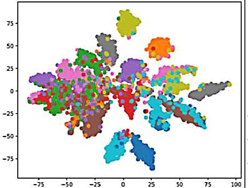
ment representations of the 20NG dataset learned Aditya Grover, Aaron Zweig, and Stefano Ermon.
by our model, DHTG and TextGCN in Figure 5, 2019. Graphite: Iterative generative modeling of
in which each dot represents a document and each graphs. In ICML, pages 2434–2444.
color represents a category. Our method yields the Arman Hasanzadeh, Ehsan Hajiramezanali, Krishna
best clustering results compared with the others, Narayanan, Nick Duffield, Mingyuan Zhou, and Xi-
which means the topics are more consistent with aoning Qian. 2019. Semi-implicit graph variational
pre-defined classes. It shows the superior inter- auto-encoders. In NIPs.
pretability of our method for modeling the latent Lianzhe Huang, Dehong Ma, Sujian Li, Xiaodong
topics along with both word co-occurrence graph Zhang, and Houfeng Wang. 2019. Text level graph
and document-word graph when compared with neural network for text classification. arXiv preprint
arXiv:1910.02356.
DHTG.
Armand Joulin, Edouard Grave, Piotr Bojanowski, and
5 Conclusion Tomas Mikolov. 2016. Bag of tricks for efficient text
classification. arXiv:1607.01759.
In this paper, we proposed a novel deep latent vari- Yoon Kim. 2014. Convolutional neural networks for
able model T-VGAE via combining the topic model sentence classification. In EMNLP, pages 1746–
with VGAE. It can learn more interpretable rep- 1751.
resentations and leverage the latent topic seman-
Diederik P Kingma and Max Welling. 2013. Auto-
tic to improve the classification performance. T- encoding variational bayes. arXiv preprint
VGAE inherits advantages from the topic model arXiv:1312.6114.
and VGAE: probabilistic interpretability and effi-
DP Kingma and JL Ba. 2015. Adam: A method for
cient label propagation mechanism. Experimental stochastic optimization. In ICLR.
results demonstrate the effectiveness of our method
along with inductive learning. As future work, it Thomas N Kipf and Max Welling. 2016. Variational
graph auto-encoders. arXiv:1611.07308.
would be interesting to explore better-suited prior
distribution in the generative process. It is also Thomas N Kipf and Max Welling. 2017. Semi-
possible to extend our model to other tasks, such as supervised classification with graph convolutional
networks. In ICLR.
information recommendation and link prediction.
Pengfei Liu, Xipeng Qiu, and Xuanjing Huang. 2016.
Acknowledgments Recurrent neural network for text classification with
multi-task learning. In IJCAI, pages 2873–2879.
This research is supported by the CSC Scholarship AAAI Press.
offered by China Scholarship Council. We would Xien Liu, Xinxin You, Xiao Zhang, Ji Wu, and Ping Lv.
like to thank the anonymous reviewers for their 2020. Tensor graph convolutional networks for text
constructive comments. We thank MindSpore for classification. AAAI.
the partial support of this work, which is a new 1
https://www.mindspore.cn/
4226Yishu Miao, Lei Yu, and Phil Blunsom. 2016. Neural Liang Yang, Fan Wu, Junhua Gu, Chuan Wang, Xi-
variational inference for text processing. In ICML, aochun Cao, Di Jin, and Yuanfang Guo. 2020.
pages 1727–1736. Graph attention topic modeling network. In WWW,
pages 144–154.
Shirui Pan, Ruiqi Hu, Guodong Long, Jing Jiang, Lina
Yao, and Chengqi Zhang. 2018. Adversarially regu- Liang Yao, Chengsheng Mao, and Yuan Luo. 2019.
larized graph autoencoder for graph embedding. In Graph convolutional networks for text classification.
IJCAI, pages 2609–2615. In AAAI.
Hao Peng, Jianxin Li, Yu He, Yaopeng Liu, Mengjiao Haopeng Zhang and Jiawei Zhang. 2020. Text graph
Bao, Lihong Wang, Yangqiu Song, and Qiang Yang. transformer for document classification. In Proceed-
2018a. Large-scale hierarchical text classification ings of the 2020 Conference on Empirical Methods
with recursively regularized deep graph-cnn. In in Natural Language Processing (EMNLP), pages
WWW, pages 1063–1072. 8322–8327.
Min Peng, Qianqian Xie, Yanchun Zhang, Hua Wang, Yufeng Zhang, Xueli Yu, Zeyu Cui, Shu Wu,
Xiuzhen Jenny Zhang, Jimin Huang, and Gang Tian. Zhongzhen Wen, and Liang Wang. 2020. Every
2018b. Neural sparse topical coding. In Proceed- document owns its structure: Inductive text classi-
ings of the 56th Annual Meeting of the Association fication via graph neural networks. arXiv preprint
for Computational Linguistics (Volume 1: Long Pa- arXiv:2004.13826.
pers), pages 2332–2340.
Yuhao Zhang, Peng Qi, and Christopher D Manning.
Dinghan Shen, Guoyin Wang, Wenlin Wang, Mar- 2018. Graph convolution over pruned dependency
tin Renqiang Min, Qinliang Su, Yizhe Zhang, Chun- trees improves relation extraction. In EMNLP,
yuan Li, Ricardo Henao, and Lawrence Carin. pages 2205–2215.
2018. Baseline needs more love: On simple word-
embedding-based models and associated pooling Qile Zhu, Zheng Feng, and Xiaolin Li. 2018.
mechanisms. arXiv:1805.09843. Graphbtm: Graph enhanced autoencoded variational
inference for biterm topic model. In EMNLP, pages
Akash Srivastava and Charles Sutton. 2017. Au- 4663–4672.
toencoding variational inference for topic models.
arXiv:1703.01488.
Ngo Van Linh, Tran Xuan Bach, and Khoat Than. 2020.
Graph convolutional topic model for data streams.
arXiv, pages arXiv–2003.
Shikhar Vashishth, Manik Bhandari, Prateek Yadav,
Piyush Rai, Chiranjib Bhattacharyya, and Partha
Talukdar. 2019. Incorporating syntactic and seman-
tic information in word embeddings using graph con-
volutional networks. In ACL, pages 3308–3318.
Petar Veličković, Guillem Cucurull, Arantxa Casanova,
Adriana Romero, Pietro Liò, and Yoshua Bengio.
2018. Graph attention networks. In ICLR.
Guoyin Wang, Chunyuan Li, Wenlin Wang, Yizhe
Zhang, Dinghan Shen, Xinyuan Zhang, Ricardo
Henao, and Lawrence Carin. 2018. Joint embed-
ding of words and labels for text classification.
arXiv:1805.04174.
Zhengjue Wang, Chaojie Wang, Hao Zhang, Zhibin
Duan, Mingyuan Zhou, and Bo Chen. 2020. Learn-
ing dynamic hierarchical topic graph with graph con-
volutional network for document classification.
Qianqian Xie, Jimin Huang, Pan Du, Min Peng, and
Jian-Yun Nie. 2021. Graph topic neural network
for document representation. In Proceedings of The
Web Conference 2021.
Xiaohui Yan, Jiafeng Guo, Yanyan Lan, and Xueqi
Cheng. 2013. A biterm topic model for short texts.
In Proceedings of the 22nd international conference
on World Wide Web, pages 1445–1456.
4227You can also read