Inferring the drivers of language change using spatial models
←
→
Page content transcription
If your browser does not render page correctly, please read the page content below

Inferring the drivers of language change using
                                                                    spatial models
                                                                         James Burridge1 and Tamsin Blaxter2
arXiv:2107.02056v1 [physics.soc-ph] 5 Jul 2021

                                                       1
                                                        School of Mathematics and Physics, University of Portsmouth,
                                                                   Portsmouth PO1 3HF, United Kingdom
                                                    2
                                                      Gonville and Caius College, Cambridge CB2 1TA, United Kingdom

                                                                                          July 6, 2021

                                                                                             Abstract
                                                          Discovering and quantifying the drivers of language change is a major challenge.
                                                      Hypotheses about causal factors proliferate, but are difficult to rigorously test. Here
                                                      we ask a simple question: can 20th Century changes in English English be explained
                                                      as a consequence of spatial diffusion, or have other processes created bias in favour of
                                                      certain linguistic forms? Using two of the most comprehensive spatial datasets avail-
                                                      able, which measure the state of English at the beginning and end of the 20th century,
                                                      we calibrate a simple spatial model so that, initialised with the early state, it evolves
                                                      into the later. Our calibrations reveal that while some changes can be explained by
                                                      diffusion alone, others are clearly the result of substantial asymmetries between vari-
                                                      ants. We discuss the origins of these asymmetries and, as a by-product, we generate
                                                      a full spatio-temporal prediction for the spatial evolution of English features over the
                                                      20th Century, and a prediction of the future.

                                                 1 Modelling language evolution
                                                 Modelling the collective behaviour of systems of sentient agents, from flocks of birds
                                                 [1, 2], to economies [3], cities [4] and languages [5, 6, 7], is attractive, but not easy. To
                                                 quote Emanuel Derman [8], an early adopter of financial modelling,
                                                    In physics there may one day be a Theory of Everything; in finance and the social sciences,
                                                 you’re lucky if there is a usable theory of anything.
                                                 The problems which arise when trying to model social systems depend to some extent on
                                                 the system in question, but share a good deal in common. In many cases we have only
                                                 one realisation of the change process which we want to understand, and the data available
                                                 about the change may be sparse. Because we cannot observe the thought processes and

                                                                                                 1
motivations of the agents, we caricature them with a simple model. However, many
different models may fit observations similarly well. This problem recedes if we have
more data and more realisations, which allow us to apply Statistical Learning methods [9],
such as cross validation, to rigorously select the “best model” by maximizing its ability
to predict unseen data. If this is not possible, because we have only one realisation of
a particular change process, then another approach is to start with some simple default
theory, or null model [10], and then seek to determine whether it is sufficient to explain
observations. We may also consider an alternative model with incrementally increased
complexity and minimal additional assumptions, the aim being to understand what is
missing from the null model, while avoiding unjustified assumptions about what should
replace it.
    The broad question which interests us is: what are the processes which drive the
evolution of languages, and how should they be represented in a coarse grained spa-
tial model? A longer term aim is to be in possession of sets stochastic equations, derived
from simple assumptions about speaker-level behaviour, which describe how language
evolves over space and time, and amongst different social groups. Such equations should
calibrate to available data on the language state up until the present, then allow us to
understand historic changes, and make future predictions. Here we take a step toward
addressing these aims, by fitting a coarse grained spatial model to two large scale spatial
datasets which capture the states of various English language features at the beginning
and end of the 20th Century.
    The mathematical modelling of language evolution, often using methods of statisti-
cal physics, is now an established field. Many aspects of language change have been
studied using non-spatial models [11, 5, 12, 13, 14], and an important focus has been to
understand the replacement of one linguistic feature by another, typically following the
ubiquitous temporal S-curve [15, 16]. Such changes can be driven by numerous mecha-
nisms, including those which favour particular variants (e.g. regularization [17], social
biases [18], or exogenous factors [16]), by stochastic effects [19, 20], and by biases driven
by linguistic variation over the age spectrum [12, 13, 21, 22, 23]. In this work we allow
speakers a learning bias toward individual linguistic features, without explicitly mod-
elling any particular mechanisms which might generate this. We seek only to determine
whether some form of bias existed, given the observed changes.
    Spatial modelling of language change is a topic of growing interest [24, 25, 26, 27, 28,
7, 29, 30, 31]. Whereas non-spatial linguistic data is plentiful, detailed spatial datasets are
rarer. Their construction typically requires either large scale collaborative effort [32, 33,
34], or viral success online [35, 36, 37]. Spatial modelling presents additional challenges in
the form of greater analytical and computational complexity, particularly when matching
models to real world spatial language distributions. There is also long standing interest
within the quantitative linguistics community in the statistical analysis of spatial, social
and temporal variations within real linguistic domains [34, 38, 39].
    Recent spatial models [7, 29, 30, 31], which accurately model geography and popula-
tion distributions, suggest that the shapes of linguistic domains and the locations of cities
and towns can have a partially predictable influence on the evolution of language. In
fact, the importance of geography has been well known to dialectologists for a long time
[18, 40]. From a mathematical perspective, this influence arises from the impact of ge-

                                              2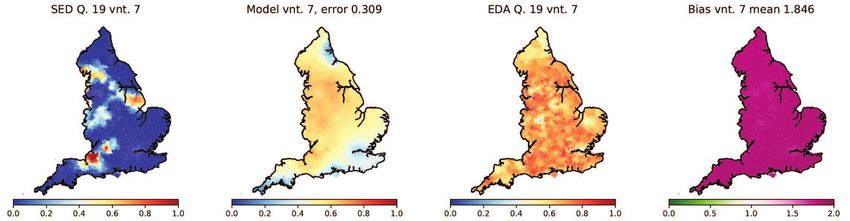
ography on the shapes of boundaries (isoglosses) between alternative linguistic features,
which behave like two dimensional bubbles. The existence of this surface tension effect
has recently been tested using historical English dialect data [31]. We therefore believe
that space and spatial processes must be part of models which seek to understand lan-
guage change processes. Here we provide, to our knowledge, the first detailed spatial
model which matches the evolution of real linguistic features within an extended spatial
domain (England in the 20th Century), accounting for realistic migration patterns, and
plausible learning behaviour.

2 Data and existing theories
2.1 Linguistic variables and variants
For the purpose of academic study, languages may be broken down into distinct com-
ponents: single units of sounds (phones), rules for combining sounds (phonology), words
(the lexicon), rules for word construction (morphology), and rules for sentence construction
(syntax). A language may be viewed as a complete specification of all its components,
and language change as the process of progressively exchanging components for alterna-
tives. We refer to a language feature for which there are a set of alternatives as a variable,
and to the alternatives as variants. These might be different words for the same object
or idea, different sounds playing the same role in certain groups of words, or alternative
syntactic rules. As an example, the word for the season after summer historically had
variants autumn, backend and fall in England [32]. The fundamental quantities which we
build models of are the relative usage frequencies of variants at different locations (or
regions) in space. Simultaneous spatial variations in many linguistic variables can create
distinctive regional dialects.

2.2 The Survey of English Dialects and the English Dialect App
We model the spatial evolution of a set of linguistic variables over the 20th Century in
England, the largest and most densely populated nation within the British mainland. As
initial and final conditions, we use data for the same variables from two surveys: the
Survey of English Dialects (SED) [41] and the English Dialects App (EDA) [35, 36].
    The SED was carried out in the 1950s at 313 localities. With 986 respondents, it is a
small survey by modern standards. The localities were selected to provide a relatively
evenly-spaced sample across England, but included almost no speakers from urban ar-
eas. This was a deliberate choice; the survey sought out the most conservative demo-
graphic (typically farm-labourers born in the 1870s and 80s) to capture the network of
“traditional” dialects before they disappeared. Methodologically, the SED was rigorous,
making few allowances for speed or convenience at the expense of data volume and qual-
ity: fieldworkers visited respondents in person and recorded their responses to over a
thousand questions in narrow phonetic transcription (and later also on tape). Despite
some criticisms arising from systematic differences in how fieldworkers asked questions
or transcribed responses [42, 43], the SED is a rich and relatively trustworthy source of

                                              3
data and has provided the material for more than half a century’s worth of secondary
analysis.
    The EDA represents a new generation of dialect data collection methods, using digital
technologies to reach a large number of respondents very cheaply. Over 50,000 speak-
ers answered 26 questions about their usage through a smartphone app in 2016, and all
but one question duplicated variables surveyed in the SED. The EDA exemplifies a dif-
ferent set of trade-offs between data quality, quantity and speed. It is possible to mine
the SED data for patterns across many responses and examine variables which were not
specifically targeted, whereas the EDA required speakers to decide between predefined
categories, limiting analysis to 26 variables and predetermined sets of variants. Instead,
the EDA’s major advantage is its 45,287 speakers in 39,590 locations within the region
covered by the SED. It is also more representative, covering urban areas and all demo-
graphics, although, because it was carried out via smartphones, it is somewhat skewed
towards younger and more affluent speakers.
    In spite of methodological differences, we argue that comparison of the SED and EDA
is a viable way to explore language change in 20th century English English. Laboratory
perception tests [36] suggest that speakers are largely able to discriminate between the
variants of the phonetic variables elicited in the EDA. Spatial patterns in the results of
the EDA, when compared to the SED, show that levelling (loss of variants) and isogloss
(linguistic boundary) movements are in line with our prior understanding of the mech-
anisms of language change. However, because typical SED respondents were old, while
EDA respondent were younger, we are not simply mapping the 60 or so years of language
change between the median dates of the two language surveys. If we assume that speak-
ers’ linguistic norms are set early in life and change little in adulthood (the underlying
assumption of much historical linguistic [44] and sociolinguistic [45] work on language
change), the relevant comparison is instead speakers’ dates of birth: the median date of
birth is the 3rd of May 1881 for SED respondents, and the 20th of July 1983 for EDA
respondents, implying that we are looking at around 100 years of change.
    Because urban areas are under-represented in the SED, we must consider whether
city varieties are likely to have differed substantially from the varieties in the regions sur-
rounding them. In that case SED maps would be missing islands of highly divergent
usage in places where spatial models [7, 29, 30] suggest that population density gradients
should preserve those distinctions or encourage the spread of urban variants. However,
the rapid urbanisation of the industrial revolution had started only a couple of genera-
tions before the SED speakers were born; less than the three generations required for new
dialect formation, according to standard models [46], and certainly not long enough for
urban varieties to have substantially diverged from their regional inputs. This is borne
out by evidence. For example, Coates [47], surveying research on traditional Bristol En-
glish, notes: “what can be shown to distinguish Bristolian at all linguistic levels from
other dialects of the region is relatively little”. Clearly city varieties at the time of the SED
will have had distinguishing features, just as varieties at any point in space differ in some
ways from those nearby; but we can assume that they tended to agree in most respects,
and so their omission is not likely to be any more problematic than a situation where any
other location happened to be lacking in samples.

                                               4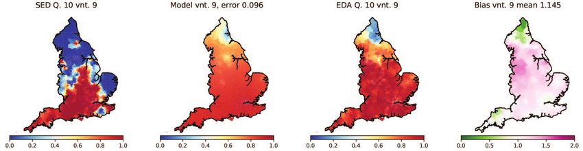
2.3 Current hypotheses about linguistic changes
The overwhelming story of change in English English dialects over the 20th and early
21st centuries is one of loss of diversity. In the words of Britain [48]:
    There has been such considerable and ongoing dialect attrition that the language use reported
across the country by Ellis’s survey of 1889 seems, in many cases and in many places, quite alien
to that spoken just over one hundred years later.
In place of smaller traditional dialects we find distinctions at larger, regional levels [49,
50, 51], and much research has focused on these regiolects and the processes of regional
dialect levelling [52, 53, 54, 55, 49] which generated them. Reductions in geographical
linguistic differences are not only due to convergence to one of several local variants but
also to geographically widespread adoption of common innovations [50]. These changes
are part of a near-universal pattern across the traditional varieties of Europe [56, 57, 58].
    It is believed that interactions between individuals can lead to a decline in linguis-
tic variation via accommodation, where conversation partners adjust their speech to better
match each other, and by child learners acquiring accommodated forms [59, 60, 61, 62, 63].
However, in certain social contexts, children may also learn variants directly from mobile
outsiders [64]. The fact that accommodation is mediated through interactions between
speakers has lead some linguists to conclude that the primary drivers in the decline of
linguistic diversity are travel, commuting and migration [59, 65, 49, 55, 66, 50, 67]. Other
potential drivers discussed include changes in social network structure [59, 68, 65, 49, 50,
55, 66], the age structure of the community [69], the influence of mass media [58, 70],
normative attitudes and education [71, 72, 58] and relatedly the salience and stereotype
status of particular variants [73, 55], identity factors [74], the informalisation of public life
[58] and socio-economic forces [55]. Purely linguistic internal factors such as structural
regularity, functional economy, or naturalness may determine which variants win out in
the levelling process [59, 67, 49, 55] or they may not be relevant at all [71, 50]. Arguments
have also been made for the central importance of idealogical factors, in particular strong
normative attitudes towards the standard, alongside mobility and contact [74, 72, 75]; par-
allel to these arguments, it has been suggested that strong alignment of speaker identities
with the local community may be enough to check the levelling process and so preserve
a distinct local variety [58, 51].
    There are clearly numerous potential drivers of linguistic change, and it is beyond the
scope of this work to quantify their relative importance. It may be that driving processes
which operate in different ways at small scales (at the level of motivations, interactions
and contacts between individuals) yield similar or identical terms in evolution equations
for coarse grained population averages, making the task of inferring the importance of
individual effects impossible using such models. However, macroscopic models have
been used to infer different classes of driving mechanism from non-spatial linguistic time
series, specifically exogenous (population level) vs endogenous (individual level) drivers
[16]. We take a similar approach here, but our two classes are spatial processes (migration,
movement), and processes which introduce asymmetry with respect to variants (ideology,
internal linguistic effects, social prestige, normative bias toward a standard etc.). We do
this by defining coarse grained evolution equations which account for both movement

                                               5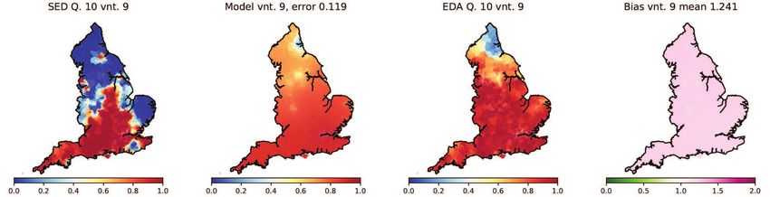
and biased copying. We then fit our model to the initial and final conditions supplied
by the SED and EDA data, to determine the relative importance of each process. Since
movement is often viewed as the primary driver of change, we view variant symmetric
dynamics as our null model, and determine the extent to which it can explain the ob-
served changes, before breaking variant symmetry by allowing for biasing factors.

3 The model
We consider a spatial domain divided into L cells, each containing (approximately) N
speakers. The centroids of these cells are written r1 , r2 , . . . , rL . Consider a linguistic vari-
able with q ∈ {1, 2, . . .} variants, and let the relative frequencies with which these variants
are used within cell r define the frequency vector f(r) = (f1 (r), . . . , fq (r))T ∈ ∆q , where
∆q is the q-dimensional simplex and T denotes transpose. We have suppressed time de-
pendence for brevity. The cells we use in our analysis are Middle Layer Super Output
Areas (MSOAs), a set of L = 7, 201 geographical polygons, each with a similar num-
ber of residents, used for reporting census data in England and Wales [76]. The mean
MSOA population in 2011 was 7, 787, and the modal area of English MSOAs is approx-
imately 0.29km2 , corresponding to a few tens of streets within a densely populated city.
Interactions with areas outside the English borders, for which we lack survey data, are ne-
glected. We justify this simplification on the basis that population densities are low at the
Scottish and Welsh borders, the English make up the great majority (≈ 87%) of the British
mainland population, and Wales and Scotland possess distinctive cultural and linguistic
identities. We assume that much longer range interactions, for example from American
TV, cinema, and music, will be subsumed into biases in the learning function (see section
3.3) which determines the adoption probabilities of different variants by young speakers.

3.1 The language community
We refer to the language that a speaker is exposed to as their linguistic environment, and
assume this environment consists predominantly of voices from their own and nearby
cells. We allow for biasing factors by weighting the influence of variants using a set of bi-
ases which affect the learning process (see section 3.3). We capture the local environment
of a speaker in cell r using the community influence matrix, W , where W (r, r′ ) gives the
influence that speakers from r′ have on speakers from r. The matrix is stochastic, meaning
that it is square with unit row sums. We define the community frequency vector of a variable
as follows                                 X
                                   bf(r) ,   W (r, r′ )f (r′ )                            (1)
                                              r′

where , denotes a definition. We assume that local influence strengths are mediated by
two factors: physical separation, and population distribution. A definition which incor-
porates both is                                            ′ 2
                                               exp − |r−r
                                                        2σ2
                                                            |
                                        ′
                                 W (r, r ) = P                    ,                            (2)
                                                         |r−r′′ |2
                                              r′′ exp  −   2σ2

                                                   6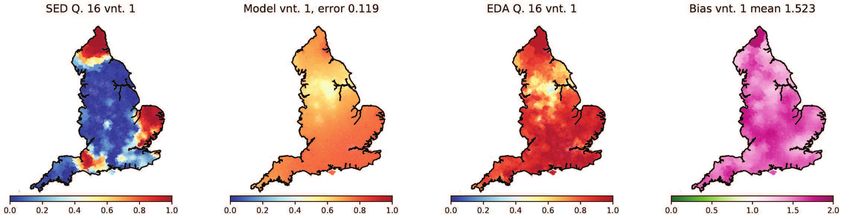
(x)
          0.15             Birmingham                 Coventry

                                                                        ˜
          0.10                                                          W(-15,x)
                                                                        ˜
                                                                        W(0,x)
          0.05                                                          ˜
                                                                        W(15,x)

          0.00
                           -20                0               20               40
                                                  x(km)

Figure 1: Effects of towns and cities on the spatial distribution of the 1D continuum in-
fluence kernel W̃ (x0 , x), given by (3). Brown curve is proportional to population density.
Coloured curves show the influences on speakers in the city centres and at the midpoint,
when the interaction range is σ = 10km.

where we call σ the interaction range. To illustrate the competing effects of interaction
range and population distribution we consider the one dimensional small-cell limit of the
influence matrix, which takes the form of a kernel giving the influence of location x on
location x0
                                                     (x−x0 )2
                                          ρ(x) exp − 2σ2
                          W̃ (x0 , x) = R                                            (3)
                                                    (y−x0 )2
                                          ρ(y) exp − 2σ2       dy

where ρ(x) is population density at x, inversely proportional to cell size at this position.
Population density is automatically accounted for in definition (2) because higher den-
sity areas have more cells. Figure 1 shows the spatial distribution of influences on three
speakers who live in or between two cities with radii and separation similar to Birming-
ham (population ≈ 106 ) and Coventry (population ≈ 3 × 10⁵ ). Consider a speaker in
central Coventry (x0 = 15). Most of the influence on them comes from within the city,
because there are relatively few people to interact with outside. This makes their effec-
tive interaction range smaller. A speaker in central Birmingham (x0 = −15) will have a
wider range of influence because their city is larger. For a speaker in between the two
cities (x0 = 0), influence comes from both, with the larger city dominating (see blue curve
in Figure 1). In the limit of very large cities (or other regions of approximately uniform
population density) the influence distribution becomes normal so that ≈ 63% of influence
comes from within σkm.
    We assume that speakers’ linguistic states are fixed in their youth (see section 3.3),
so the interaction range should be chosen to capture the community state observed by a

                                             7
younger speaker. An empirical measure of such separations is provided by school travel
distances; secondary education has been compulsory since 1918, so we would expect chil-
dren to regularly interact with others from their school catchment. In the early 21st cen-
tury secondary pupils travelled, on average, ≈ 5.5km to school [77]. We will call this
the mean catchment radius, denoted µR . The number of state schools has declined some-
what over the 20th century; in 1951 there were 5,900 vs. 4,072 in 2010 [78]. This implies
that average catchment radii have increased, with 1951 radii being ≈ 83% early 20th cen-
tury radii. Scaling 2010 travel distances by this factor yields an average travel distance of
≈ 4.5km. Suppose we model the distribution of displacements between home and school
as a bivariate normal distribution
                                                  x2 +y 2
                                                 e− 2ω2
                                      f (x, y) =         ,                                 (4)
                                                  2πω 2
                                                  p
then the mean home-school distance is µR = π2 ω and the mean distance between two
                   q
                      8
homes is 2ω =           µ ≈ 1.6µR . This suggests a typical distance between interacting
                      π R
speakers is between 5 and 10km. Since σ functions as an upper bound in cities, we take
our interaction range as the upper limit of this interval, so σ = 10km ≈ 6miles.
    We assume that speakers from a given cell have similar environments, so that bf(r) ap-
proximates the perceptions of all speakers in zone r. The assumption that all the speakers
in a cell access the same primary linguistic data is a simplification of reality. We know that
within many geographical areas there are subgroups whose language differences may de-
pend on class, sex or ethnicity [18]. We simplify in this way because we are interested in
national level spatial variations for which we have detailed geographical data, but no
consistent breakdown by social subgroup, so cannot infer any effects of subgroups. We
implicitly assume that social subgroups can induce biases on variants.

3.2 Migration
Migratory processes may be internal, where individuals move between locations in a sin-
gle language area (typically a country), or external, where they arrive from another coun-
try or language area. During the 20th Century, foreign-born people have made up a small
and slowly changing percentage of the English population; 4.2% in 1951, for example,
rising to 6.7% in 1991 [79]. The cumulative total number of migrants to Britain from the
early 1800s to 1945 is estimated as 2.34 million [80]. Since numbers are small, we do
not explicitly model external migration, instead viewing it as one of many possible fac-
tors which may induce biases. To model internal migration, we need to know how often
people move, and how far. The English Longitudinal Survey of Ageing (2007), showed
that for individuals aged 50-89, the average number of different residences occupied for
at least six months during their lifetime was 5.6 for those born 1918-1927, rising to 6.42
for those born 1948-1957 [81], giving an average of approximately one move every ten
years. Inter-county migration distances may be extracted from birthplace and place of
residence recorded in censuses, providing data back to the mid nineteenth century [82].
Such data is, however, spatially coarse; it provides no information about short range mi-
grations. Modern lifestyle survey data can help fill the gap. Analysis [83] of large scale

                                              8
research polls by Acxion Ltd (2005-2007), which recorded current and previous postcode,
generated ≈ 1.25 × 10⁵ migration distances, having mean 25.77km, median 2.89km and
standard deviation 63.91km. This implies a migration distribution concentrated at short
distances, with sub-exponential decline at large distances. This large distance migration
behaviour is often modelled with a power, or ”gravity” law [83, 84].
    Models of migration must be consistent with migration distance statistics, and con-
strained so that total flows in and out of cells match observed values. This can be achieved
[85] by writing the expected number of people who leave their address in cell r and move
to a new address in r′ as

                          m(r, r′ ) , A(r)B(r′ )O(r)D(r′ )h(|r − r′ |)                      (5)

where O(r) is the total number of movers whose previous address was in r, D(r′ ) is the
total number of people whose new address is in r′ , and h(|r − r′ |) is a distance function
which, typically, decreases for longer moves. The conditions
                                    X
                                       m(r, r′ ) = O(r)                                  (6)
                                      r′
                                      X
                                               m(r, r′ ) = D(r′ ),                          (7)
                                      r

imply that
                                                                           !−1
                                      X
                            A(r) =              B(r′ )D(r′ )h(|r − r′ |)                    (8)
                                          r′
                                                                       !−1
                                      X
                           B(r′ ) =             A(r)O(r)h(|r − r′ |)         .              (9)
                                           r

A mover might shift to a new address in the same cell, and the quantity m(r, r) gives the
expected number of people who do this within cell r. The sets of constants A , {A(rk )}Lk=1
and B , {B(rk )}Lk=1 are found by generating a sequence of sets A0 , B0 , A1 , B1 , . . . where
A0 is the set for which A(r) = 1 for all r, Bk is computed from Ak using (9), and Ak+1 is
computed from Bk using (8). The sequence is then iterated to convergence.
   We assume that our cell populations are in equilibrium and without loss of generality
assume there is one mover per cell, so O(r) = D(r) = 1, and m(r, r′ ) is a stochastic matrix
with elements which represent transition probabilities for a single mover. The matrix can
be rescaled to capture realistic migration rates. We define the distance function
                                                   2
                             h(r) = ωe−(r/a) + 1{r>0} (1 − ω)r −ρ                         (10)

where the first term models short range moves with typical range a, and the second term
is the long distance fat-tail of the distribution, with gravity exponent ρ. The parameter
ω ∈ [0, 1] interpolates between entirely short range, and pure power law distributions.
Having calculated m(r, r′ ) for our system, the cumulative distribution of the migration

                                                       9
Figure 2: Cumulative distribution of migration distances generated using distance func-
tion (10) with ω = 0.75, a = 3km and ρ = 1.5. The mean, median and standard deviation
are 31.3km , 3.6km and 63.4km respectively. For comparison, the corresponding statis-
tics computed from Acxion survey data [83] are 26.3km, 3.6km, and 63.7km. Horizontal
dashed lines show the fraction of moves less then ten miles (71%) and fifty miles (87%).
distance X is calculated as
1 X X √
P(X < r) = H (r − |r − r ′
|) m(r, r ′
) + H r − R(r)/ 2 m(r, r) (11)
L r,r′
r
r6=r′
where H is the Heaviside step function and R(r) is the radius of a circle with identical
area to cell r. The second term√ in the square brackets accounts for all intra-cell moves, as-
sumed to be of distance R(r)/ 2, following [86]. We select distance function parameters
to match the short range (median) and long range (standard deviation) statistics of the
inter- and intra-cell distance distribution computed in [83] for MSOAs, using the Acxion
data. This was achieved by parameter grid search to minimize the sum of the relative er-
rors in the median and standard deviation between the model and the Acxion data. The
resulting distribution (Figure 2) is our estimate for migration distances at the turn of the
21st century. Its shape reflects two kinds of migratory events: frequent short moves, per-
haps to change accommodation, and rarer long distance moves, leaving behind friends,
work and other social contacts, where the distance travelled becomes relatively less sig-
nificant.
We now consider whether this distribution may be used to approximate migration
during in earlier periods. Increased move frequency over the 20th century does not imply
that the distribution of distances has also changed. Although we lack detailed informa-
tion about historical short range moves, we can compare our distribution to statistics of
10Figure 3: Yearly percentage changes in population for English and Welsh counties, av-
eraged over 1851-1951, calculated from the census based estimates of Friedlander [82].
Counties with the highest and lowest average rates of change are labelled.
longer migrations extracted [87] from the National Marriage and Fertility survey (1959-
1960), which sampled more than 2000 couples aged 16-60. The survey showed that 16%
of moves were of 10-49 miles and 15% were 50 miles or more. Our corresponding per-
centages are 16% and 13% respectively (Figure 3). The similarity of these estimates, and
the sample error associated with historical percentages (estimated at ±1%), suggests that
the statistics of long distance internal migrations have not changed dramatically. Because
people are most likely to migrate in their mid twenties [81], many of the moves in the
1959-1960 marriage survey may have been made much earlier in the century.
We also consider whether our assumption that each cell is in equilibrium is reason-
able. Using estimates of net inter-census population changes calculated by Friedlander
[82] for counties in England and Wales, we have computed the yearly percentage popu-
lation change by county, averaged over 1851-1951 (Figure 3). The results show south east
England experienced the greatest inflow of migrants, and that the root mean squared net
flow rate over all counties is ≈ 0.45%. By comparing this figure with the overall yearly
migration rate of ≈ 10% we see that, on average, in cells that are gaining, for every 20
people who leave, 21 will arrive. Since net changes in population are therefore typically
at least an order of magnitude smaller than than absolute population flows, we assume
that non-equilibrium effects can be ignored.
Long range migration in principle allows variants to jump between locations within
the spatial domain. This jumping process is the subject of the linguistic gravity model [88,
18], which attempts to quantify the spread of variants between a finite set of population
centres, viewed as points in space. In contrast, the cells in our model cover the entire
spatial domain, and population centres appear as densely packed clusters. Other than cell
size, there is no intrinsic difference between city and rural cells. The effects of allowing
11city speakers to behave differently to their rural counterparts, in a spatial model similar
to ours, was explored in [29], along with connections to other classical models of spatial
linguistic spread including the wave model and hierarchical diffusion [89, 40].
3.3 Language learning and evolution
We assume an iterative model of language evolution, in which dying adults are replaced
by new speakers who select a variant using the probability mass function
p(r) , g b f (r) (12)
where g : ∆q → ∆q is the learning function. An alternative interpretation, which yields
dynamics which have identical deterministic component, but no stochasticity, is that the
components of p(r) give the relative frequencies with which new speakers use different
variants. We could, if we wished, interpolate between these two interpretations by as-
suming a mixture of the two behaviours. In either case equation (12) captures the learning
process which converts infants into adult speakers. It is an approximation of the cumu-
lative effect of countless small iterations made within a changing learning environment.
Underlying this model is the assumption that linguistic behaviour is mainly acquired in
childhood, and changes little in later life. Learning to speak requires the assimilation
of a variety of structures, from sets of individual sounds and sound patterns, through
words and morphological rules, to syntax. Learning processes differ between structures,
and we do not aim to capture these processes in detail. Rather we propose a simple but
plausible learning function which maps current speech patterns to learned forms. We de-
rive evolution equations by considering the case which generates maximum stochasticity:
where new speakers select a single variant. We will then consider the importance of this
stochasticity.
A simple learning model, analogous to neutral evolution in genetics [90, 91, 92, 5, 14], is
that variants are selected with a probability equal to their current frequency. This has two
problems as a model of language evolution. First, as we will show below, linguistic com-
munities would take an extraordinarily long time to settle on one feature. Second, the
geographical boundaries between language features (isoglosses) revealed by linguistic
surveys, appear to require some form of social conformity [7, 29, 31] meaning that speak-
ers preferentially select the most common variants with a probability which exceeds their
relative frequency. Such a selection strategy is optimal if advantage can be gained by
matching the speech of others. We can incorporate both conformity and asymmetric bias
toward different variants by defining the learning function
hk f β
[g(f)]k , Pq k β (13)
i=1 hi fi
where [f]k denotes the kth component of the vector f ∈ ∆q . The variables hk > 0 are
biases, and β ≥ 1 is the conformity number. If β > 1 then g(f) increases the frequencies
of already popular variants, and reduces the frequencies of less popular ones. The biases
h1 , . . . , hq , which we write as a vector h, introduce variant asymmetry, with the selection
12probability of the kth variant an increasing function of hk . However, g(f ) is invariant
under a constant re-scaling of all biases so it is their ratios which determine the extent to
which variants are favoured.
To derive equations for the evolution of frequencies, we denote the counts of speakers
using the variants of a given linguistic variable within cell r at discrete time step t as
X(r, t) = (X1 (r, t), . . . , Xq (r, t))T (14)
where q
X
Xi (r, t) = N. (15)
i=1
We model renewal (birth and death), and migration. At each time step, nR adults die and
are replaced with young speakers, and nM migrate. The renewal and migration rates are
nR
λR , (16)
N
nM
λM , . (17)
N
We set λM = 0.1, corresponding to one migration per decade, and λR = 0.02 correspond-
ing to a typical period of 50 years between reaching linguistic maturity, and leaving the
language community. We justify this latter estimate on the basis that linguistic matu-
rity occurs in the late teens [93], and that UK life expectancy in the mid 20th century
was in the late sixties [94]. The total number of speakers who die or migrate in each
cell is n , nR + nM . These speakers are selected uniformly at random from the existing
population, implying that both lifetimes and times between migrations are geometrically
distributed with parameters λR and λM , respectively.
If each migrator were to select their new cell using the symmetric transition probability
matrix m(r, r′ ), then the expected number of migrators received by each cell would be nM ,
and the expectation of the mean linguistic state of the migrators incident on cell r would
be X
m(r′ , r)f(r′ , t) , f̄(r, t). (18)
r′
We model migration by replacing our nM migrators with nM speakers with states se-
lected according to the probability vector f̄(r, t). We write the variant counts of these
speakers XM (r, t) ∼ multinomial(nM , f̄(r, t)). The variant counts of the speakers who
replace the dead is a random variable, XR (r, t) ∼ multinomial(nR , p(r)). The variant
counts of the speakers who die or migrate is a random variable, Y(r, t), drawn from the
multi-hypergeometric distribution [95] with parameters (n, X(r, t)). The change in vari-
ant counts between t and t + 1 is then
∆X(r, t) = XR (r, t) + XM (r, t) − Y(r, t) (19)
where ∆X(r, t) , X(r, t + 1) − X(r, t). Dividing by N, we have
∆f (r, t) = E[∆f (r, t)] + (∆f(r, t) − E[∆f (r, t)]) (20)
= λR g bf(r, t) − f (r, t) + λM f̄(r, t) − f(r, t) + ∆Z(r) (21)
13where ∆Z(r) , ∆f (r, t) − E[∆f (r, t)] is a zero mean noise term. The variance of the kth
component of this term, using the properties of the multinomial and multi-hypergeometric
distributions, and suppressing r dependence for brevity, is
1 λ(1 − λ)
V[∆Zk ] = λR pk (1 − pk ) + λM f¯k (1 − f¯k ) + fk (1 − fk ) (22)
N 1 − N −1
where λ , λR + λM . The magnitude of the stochastic element of cell dynamics therefore
scales as N −1/2 . For reasons set out below, we assume ∆Z(r) ≈ 0, in the current paper.
3.4 The importance of noise
To explore the significance of the noise term in (21), we consider a small, well connected
community where linguistic evolution is neutral [96, 90, 91], meaning that new speak-
ers adopt variants with probabilities equal to their relative frequencies, so p(r) = f(r).
In the case of a binary variable, the relative frequency of variant 1 admits the diffusion
approximation [97] r
2λR p
df = f (1 − f )dWt (23)
N
where Wt is a standard Brownian motion [98]. Equation (23) is known as the Wright-
Fisher diffusion [97] and describes the evolution of the relative frequency of one of two
variants (alleles) of a gene in a haploid organism. Notice that the evolution is driven
entirely by noise in this case. Let T be the time taken for the cell population to settle on
one variant (f = 0 or 1). This is the fixation time. Starting from the initial condition f = 12 ,
we have
N
E[T ] = ln 2. (24)
λR
To be concrete, let us consider the case where N is the average population of a single cell
(N = 7, 787) in our model, equivalent to a 0.25km2 block of city streets. Using λR = 0.02
(as above) we have E[T ] = 269, 877 years. From this we see that even in a relatively tiny
population, the time for one variant to become dominant by noise alone is comparable to
the time for which humans have existed as a species. We therefore neglect the stochas-
tic element of our dynamics on the basis that it is inadequate to explain changes over a
plausible time scale. Many of the linguistic variants which interest us have disappeared
over the course of a single century and only the deterministic terms in (21) are capable of
producing such a change.
Having decided to neglect the stochastic term in our model, we now consider whether
other forms of stochasticity could explain the observed changes. We have assumed our
small community is “well connected”, meaning that all learners are exposed the same
inputs. Suppose instead that children learn variants from only a small subset of the com-
munity. This effectively subdivides the population into smaller groups (e.g. families)
within which variants are reproduced by neutral selection, and between which individu-
als are exchanged (e.g. by marriage). Such processes are studied in models of neutral ge-
netic evolution in subdivided populations, such Wright’s island model [99], and Kimura’s
14stepping stone model [96, 91]. At low exchange rates between groups, the time to fixa-
tion increases relative to the fully mixed (single group) case. At sufficiently high mixing
rate the population becomes effectively panmictic, and fixation time statistics match the
fully mixed case. Subdividing the population therefore does not change our decision to
neglect the stochastic term in our model. One way for unbiased random copying to be
a more powerful driver of change is via the topology and dynamics of the social contact
network [92]. For example, if it is strongly clustered then certain individuals or groups
become particularly influential. Another possibility is that variants spontaneously gain
linguistic momentum [21, 12, 100] starting from small stochastic fluctuations. We do not
rule out either possibility, but emphasize that stochasticity as we have modelled it is in-
consequential in large populations. This does not mean that we think language change is
deterministic. Rather, unpredictable driving forces must result from factors which are not
part of our model. Whether their origin is stochastic momentum-like effects, social net-
work dynamics, internal linguistic biases or societal changes outside the linguistic system,
they all exert an effective bias (real or apparent) on language change, but in a direction
that cannot be known in advance. We can view these factors as random variables whose
values are realised as history unfolds. Having observed our linguistic system’s histori-
cal state, we can then ask: how strong must these biases have been, acting in combination
with migration, mixing and social conformity, to produce today’s language distributions?
Having established which variants require bias in our simple model, we can then turn to
understanding their origin.
3.5 Interpreting model parameters
Our deterministic evolution equation
b
∆f(r, t) = λR g f(r, t) − f(r, t) + λM f̄(r, t) − f(r, t) (25)
models four processes, two spatial, two not. The two right hand terms are the replacement
term, with rate constant λR , and the migration term having rate λM . Mundane mobility
is represented by community matrix W (r, r′ ) in our model, which is used to compute
b
f(r, t) and migration by the matrix m(r, r′ ), used to compute f̄(r, t); the effects of these are
modulated by conformity β. Together, these represent a purely spatial, accommodation-
and diffusion-driven model which does not differentiate between variants. Factors which
might create bias (see section 2.3) are modelled with the bias vector h. If dialect change
has mostly been driven by mobility, as many scholars have suggested, we would expect
h ≈ 1. However, if linguistic factors have been crucial in selecting variants, if the stan-
dard ideology has driven levelling, or if local identity factors are important in explaining
differences between conservative and innovative regions, then h will play a more sub-
stantial role. One possibility is that bias drives the selection of the levelling target, but
that migration and other spatial factors determine the speed and course of levelling. This
would be reflected in the model by high but spatially uniform h. In such a case, bias might
reflect a linguistic constraint derived from a property common to the linguistic system at
all localities, or a near-universal social pressure (such as normative pressure from univer-
sal schooling). Alternatively, observed regional differences in levelling in the EDA data
15Figure 4: Phase diagram showing regions of (β, r) space for which D can retain variant
1 when φ1 = 0, for migration-replacement ratios, ρ = λM /λR , in the set ρ ∈ {1, 5, 20}. If a
region of the phase diagram is stable for some ρ∗ , then it is stable for all ρ < ρ∗ .
might not be explained by migration and spatial factors alone and must be modelled with
a strongly spatially varying bias. This would imply that local differences in language ide-
ologies play an important role, or that interactions between dialect features create internal
pressures varying between dialects.
4 Interaction between conformity and migration
In the absence of bias, when β > 1, then the replacement and migration terms in (25)
represent two competing processes. The replacement term moves the community toward
a single local variant, whereas the migration term pulls local forms toward the average
linguistic state in a much wider linguistic area. Before comparing our model to data, we
illustrate how it operates.
4.1 Survival of an isolated domain
We consider a binary variable, and let f(t) = (f1 (t), f2 (t))T be its relative frequency vector
within a dialect area D. Let r be the escape distance: the expectation of the distance from a
randomly chosen point in D, to the boundary of D, in a randomly selected direction. The
fraction of migrators who escape D is then approximately 1 − P(X < r) , ǫ(r) where P
is the migration measure defined in (11). By the symmetry of the migration matrix, this
is equal to the fraction of speakers who enter D. Writing φ1 for the relative frequency
of variant 1 outside D, then the average state of the migrators incident on D (including
16internal movements) will be
f¯1 = (1 − ǫ(r))f1 + ǫ(r)φ1 . (26)
| {z } | {z }
moves within D migration from outside D
The language state of D then evolves (assuming h = 1) as follows
" #
f1β
∆f1 = λR β − f1 + ǫ(r)λM [φ1 − f1 ] . (27)
f1 + (1 − f1 )β | {z }
| {z } long range levelling
local conformity
The first term generates conformity to the majority variant within D. The second gener-
ates levelling toward the external language state. Suppose that most speakers in D use
variant 1, which distinguishes them from the nation as a whole, where variant 2 is used
(so φ1 ≈ 0). The equilibria (∆f1 = 0) of (27) determine the conditions under which D will
retain its distinctive feature. Informally, we look for the values of f1 for which the rates of
conformity and levelling are in balance
|local conformity| = |national levelling|. (28)
When φ1 = 0, this condition may be written
f1β ǫ(r)λM
= 1+ f1 . (29)
f1β + (1 − f1 )β λR
An upper bound on the migration rate which allows variant 1 to persist within D is ob-
tained by considering solutions in the infinite conformity limit β → ∞ where learners
always select the majority local variant. In this case the left hand side of (29) is a unit step
at f1 = 12 , and there is a stable equilibrium f1∗ > 21 provided
ǫ(r)λM
< 1. (30)
λR
This is an intuitively reasonable condition; it says that a local distinctive feature can in
principle survive provided the rate of inward migration does not exceed the rate at which
young indigenous speakers replace dying adults. We estimate that during the 20th cen-
tury, λM ≈ 0.1. There is some flexibility in the way we interpret λR . If we consider
speakers to be members of the speech community from birth, then λ−1 R is simply life ex-
pectancy. However, if speakers are only influential once older, and cease to be so when
very old, then λ−1
R is the average of this time interval. As noted in section 3.3, we have set
λR = 0.02. What determines domain stability is not however the absolute values of the
migration and replacement rates. It is their ratio
λM
ρ, . (31)
λR
For given ρ, the stability of D can be computed for any value of β and r by checking that
the dynamics (27) has a stable fixed point f1∗ > φ1 . The phase diagram in Figure 4 shows
that for lower migration-replacement ratios smaller domains can persist for lower values
of conformity. In systems where the migration-replacement ratio grows slowly, such as
in the English dialect area in previous centuries, we would expect smaller dialect areas to
disappear as the phase boundary shifted.
17Figure 5: A 500 year simulation starting from randomized initial conditions with linearly
increasing migration rate λM (t) = 0.1 × t/500. Other parameters λR = 0.02, β = 2.5, σ =
10km.
4.2 Competition between migration and conformity in the English di-
alect area
We consider a hypothetical period of 500 years, beginning with a domain in a completely
randomised state. This state is constructed by setting the initial frequency f1 (r, 0) of each
cell to be an independent uniform random variable on [0, 1]. We allow the migration rate
to be a linearly increasing function of time, starting with zero migration and reaching late
20th century levels by end of the period
t
λM (t) = 0.1 × . (32)
500
Within a few decades, recognisable dialect domains emerge (Figure 5). These are anal-
ogous to domains in ferromagnetic materials which form because neighbouring atoms
tend to align their magnetic directions. Domain boundaries evolve as if they feel a form
of surface tension [101] which penalises curvature. In physical systems, domains grad-
ually expand as their boundaries straighten. The analogy between these magnetic do-
main boundaries, and isoglosses, was explored in detail in [7, 29], including the effects
of non-uniform population distribution. It was shown in [7] that concentrated human
settlements (villages, towns, cities) balance the surface tension effect by inducing isogloss
curvature, implying that stable isogloss shapes are partially predictable from population
18Figure 6: A 500 year simulation starting from randomized initial conditions with constant
low migration rate λM = 0.01. Other parameters λR = 0.02, β = 2.5, σ = 10km.
distributions. At low migration levels, competition between isogloss smoothing, induced
by surface tension, and curvature, induced by population distribution (as well as other
natural barriers) leads to stable geographical distributions. In Figure 5 the map obtained
after 200 years would be stable in the absence of increasing migration. This stability is
revealed in Figure 6, which shows how the system evolves starting from an initial condi-
tion which is an exact copy of that in Figure 5, but under conditions of consistently low
migration (ρ = 21 ). This shows that the pattern reached after 200 years remains stable for
the next 300 years, and includes a number of isolated dialect areas with small escape radii.
Returning to Figure 5 we see that as migration increases these small dialect areas disap-
pear, being replaced with the variant which is in the majority further afield. Eventually
the system reaches a state observed in both the SED and EDA surveys, which consists of a
major isogloss bisecting England. The stable north east dialect centred on Tyneside is also
seen in survey data. The major Wash-Severn isogloss is particularly stable because nei-
ther variant is in the majority in the country as a whole, and because it bisects the country
via one of the shortest routes. A detailed mathematical explanation of these effects, which
are related to continuum percolation, is given in [7, 29]. The north east dialect is stable
in this simulation because of its status as a dense but geographically isolated population
centre.
195 Inference for English dialects
5.1 Methodology
We now explore how our model predicts the evolution of linguistic variables which have
been recorded in both the SED and the EDA. These are listed in Table 1. For each variable
we evolve our model T = 100 years forward in time using its SED state as our initial con-
dition. To generate this initial condition from raw survey data, we set variant frequencies
in each model cell (MSOA) to match the variant frequencies from the nearest SED survey
location. If multiple variants were recorded in this location, they are assumed to all have
equal frequency. This process yields a tessellation of England into single and shared-
variant regions. Relative frequencies in each cell are then replaced with average frequen-
cies over its 20 nearest neighbours (mean separation 5.4 km). This amounts to a form of
smooth interpolation between relative frequencies observed at SED survey points, which
have typical separation ≈ 20km (calculated as square root of mean land area per location).
The resulting distribution has smooth transitions with widths typically 10-30km, consis-
tent with English transition zones discussed in Ref. [18]. While we would not expect
our results to be sensitive to the number of nearest neighbours used in the smoothing
(interpolation) step, we have avoided smoothing to a level where frequency values at
SED locations would be changed substantially in transition regions (e.g. if the smoothing
range approached the typical separation of survey locations).
We consider both bias free (h = 1) and biased evolution. We allow for the possibility
that biases may be different in different parts of the country by introducing a spatially
varying field
h(r) = (h1 (r), . . . , hq (r))T (33)
where hk (r) is the bias on variant k in cell r. We do not allow the bias field to depend
on time because we have only initial and final conditions, and cannot therefore calibrate
time dependence. We wish to fit h(r) so that the final state of our simulation, initialised
with an SED variable, closely matches the corresponding EDA data. This is achieved by
iterating the following learning step, which increases or decreases local biases on variants
which are respectively under- or over-represented in the model, when compared to the
EDA
b n+1 (r) = η(f EDA (r) − f n (r, T )) + θ(1 − hn (r)).
h (34)
Here hn (r) is the nth iteration of our bias estimate and f n (r, T ) is the frequency distribu-
tion obtained using this estimate. The learning rate, η, controls how rapidly adjustments
are made, and the reversion rate, θ, is a regularization parameter that prevents runaway
bias increases, and maintains h = 1 as the “no-bias” reference point so that calibrations
for different variables can be compared. We use the initial condition h0 (r) = 1.
To avoid over-fitting we introduce a smoothing factor, σs , which interpolates between
independent variation in bias between cells (σs = 0) and constant bias in all cells (σx →
∞). The quantity h b n+1 (r) is the new bias estimate before spatial smoothing (indicated by
the hat symbol). Having applied the learning step (34), we apply a smoothing step using
20Table 1: Questions, variables and variants for the EDA (and SED). All phonetic variants are writ-
ten using the International Phonetic Alphabet [102]. ME = Middle English
Question in the EDA Variable Variants
1. The word “tongue” can end in two Coalescence of [Ng] 1. [Ng], 2. [N]
different ways. Which do you use?
2. Which pronunciation of “new” is the yod-dropping 1. no [j], 2. [j]
most similar to your own?
3. How do you pronounce the word TRAP-BATH split 1. [A:], 2. [a:], [æ:] 3. [a], [æ]
“last”?
4. In the word “butter”, I pronounce FOOT-STRUT split 1. [U], 2. [2]
the letter “u” as...
5. Do you pronounce the “r” in “arm”? rhoticity 1. no /r/, 2. /r/
6. How do you pronounce the word realisation of word-initial 1. [T], 2. [d], [ã], 3. [f], 4. [t]
“three”? /T/
7. Do you pronounce the “r” before the intrusive /r/ 1. /r/ 2. no /r/
“-ing” in “thawing”?
8. What is the season that follows sum- autumn lexical item 1. autumn, 2. backend, 3. fall
mer?
9. How do you pronounce the “l” in l-vocalisation 1. [ë], 2. [u], [U], 3. [l]
“shelf”?
10. What do you call a piece of wood splinter lexical item 1. shiver, 2. sliver, 3. speel, 4. spelk,
stuck under your skin? 5. spell, 6. spile, 7. spill, 8. splint, 9.
splinter, 10. spool
11. How do you pronounce the word realisation of ME /o:/ in 1. [Y:], [Y], 2. [u:], 3. [U]
“room”? “room”
12. How do you pronounce the word weak vowel merger 1. [@], [2], 2. [I]
“chicken”?
13. How pronounce the word “night”? realisation of ME /ix/ 1. [AI], 2. [A:], 3. [O], [6], 4. [Ei], 5. [2i],
[@i], 6. [aI], [æI], 7. [a:], [æ:], 8. [i:]
14. He wasn’t careful with the knife initial element in 3sg m. 1. himself, 2. hisself
and managed to cut... reflexive pronoun
15. If it belongs to a woman its... 3sg f. possessive pronoun 1. hern, 2. hers
16. Do you pronounce the “h” in h-dropping 1. /h/, 2. no /h/
“hands”?
17. If you’d like someone to pass you dative alternation 1. give it me, 2. give it to me, 3. give
something, would you say: me it
18. How do you pronounce the word LOT-CLOTH split 1. [O:], 2. [A:], 3. [6]
“off”?
19. How do you pronounce the word realisation of ME /u:/ 1. [@u], [2u], [œ7], 2. [E:], 3. [Eu], 4. [aI],
“house”? 5. [a:], 6. [æu], [æ7], 7. [au], 8. [u:]
20. How do you pronounces the word realisation of ME /a:/ 1. [I@], [Ia], 2. [æI], 3. [e:], [e@], 4. [ei],
“bacon”? [Ei], [E:], [E;@]
21. How do you pronounce the word realisation of ME /i:/ 1. [AI], 2. [A:], 3. [OI], 4. [EI], 5. [2I], [@I],
“five”? 6. [aI], [æi], 7. [a:], [æ:]
22. How do you pronounce the last coda /t/ 1.[P] , 2. [d], [R] , 3. [t]
sound of “bit” when saying “a bit of”?
23. Fill in the gap: Every day on her habitual present 3sg. 1. do feed, 2. feed, 3. feeds
walk past the lake, she ... the ducks.
24. How do you pronounce the word happY tensing 1. [9], 2. [I], 3. [e], 4. [i]
“happy”?
25. An animal that carries its house on snail lexical item 1. dod-man, 2. hodmedod, hoddy-
its back is a... dod, hoddy-doddy, 3. snail
21You can also read