Integrating empirical models and satellite radar can improve landslide detection for emergency response
←
→
Page content transcription
If your browser does not render page correctly, please read the page content below
Nat. Hazards Earth Syst. Sci., 21, 2993–3014, 2021
https://doi.org/10.5194/nhess-21-2993-2021
© Author(s) 2021. This work is distributed under
the Creative Commons Attribution 4.0 License.

Integrating empirical models and satellite radar can
improve landslide detection for emergency response
Katy Burrows1,a , David Milledge2 , Richard J. Walters1 , and Dino Bellugi3
1 COMET,   Department of Earth Sciences, Durham University, Durham, UK
2 School of Engineering, Newcastle University, Newcastle, UK
3 Department of Geography, University of California, Berkeley, Berkeley, USA
a now at: Géosciences Environnement Toulouse, Toulouse, France

Correspondence: Katy Burrows (katy.burrows@get.omp.eu)

Received: 17 May 2021 – Discussion started: 19 May 2021
Revised: 25 August 2021 – Accepted: 22 September 2021 – Published: 7 October 2021

Abstract. Information on the spatial distribution of triggered      1   Introduction
landslides following an earthquake is invaluable to emer-
gency responders. Manual mapping using optical satellite            Earthquake-triggered landslides are a major secondary haz-
imagery, which is currently the most common method of gen-          ard associated with large continental earthquakes and disrupt
erating this landslide information, is extremely time consum-       emergency response efforts. Information on their spatial dis-
ing and can be disrupted by cloud cover. Empirical models           tribution is required to inform this emergency response but
of landslide probability and landslide detection with satellite     must be generated within 2 weeks of the earthquake in order
radar data are two alternative methods of generating infor-         to be most useful (Inter-Agency Standing Committee, 2015;
mation on triggered landslides that overcome these limita-          Williams et al., 2018). The most common method of gener-
tions. Here we assess the potential of a combined approach,         ating landslide information is manual mapping using optical
in which we generate an empirical model of the landslides           satellite imagery, but this is a time-consuming process and
using data available immediately following the earthquake           can be delayed by weeks or even months due to cloud cover
using the random forest technique and then progressively            (Robinson et al., 2019), leading to incomplete landslide in-
add landslide indicators derived from Sentinel-1 and ALOS-          formation during the emergency response.
2 satellite radar data to this model in the order they were            In the absence of optical satellite imagery, there are two
acquired following the earthquake. We use three large case          options for generating information on the spatial extent of
study earthquakes and test two model types: first, a model          triggered landsliding in the immediate aftermath of a large
that is trained on a small part of the study area and used to       earthquake. The first is to produce empirical susceptibility
predict the remainder of the landslides and, second, a pre-         maps, using factors such as slope, lithology and estimations
liminary global model that is trained on the landslide data         of ground shaking intensity to predict areas where landslides
from two earthquakes and used to predict the third. We as-          are likely to have occurred (e.g. Nowicki Jessee et al., 2018;
sess model performance using receiver operating characteris-        Robinson et al., 2017; Tanyas et al., 2019). The second is
tic analysis and r 2 , and we find that the addition of the radar   to estimate landslide locations based on their signal in satel-
data can considerably improve model performance and ro-             lite synthetic aperture radar (SAR) data, which can be ac-
bustness within 2 weeks of the earthquake. In particular, we        quired through cloud cover and so is often able to provide
observed a large improvement in model performance when              more complete spatial coverage than optical satellite imagery
the first ALOS-2 image was added and recommend that these           in the critical 2-week response window (e.g. Aimaiti et al.,
data or similar data from other L-band radar satellites be rou-     2019; Burrows et al., 2019, 2020; Jung and Yun, 2019; Kon-
tinely incorporated in future empirical models.                     ishi and Suga, 2019; Mondini et al., 2019, 2021).

Published by Copernicus Publications on behalf of the European Geosciences Union.
2994                  K. Burrows et al.: Integrating empirical models and satellite radar can improve landslide detection

   To generate an empirical model of triggered landslides           intensity and InSAR coherence to detect landslides triggered
following an earthquake, a training dataset of landslides is        by the 2018 Hokkaido earthquake, and Ohki et al. (2020)
analysed alongside maps of “static” factors known to in-            used random forest classification to combine several land-
fluence landslide likelihood, e.g. slope and land cover, as         slide indicators based on polarimetric SAR and topography
well as “dynamic” causative factors, e.g. ground shaking            to detect landslides triggered by two events in Japan: the
estimates, and a model is produced that predicts landslide          2018 Hokkaido earthquake and heavy rains in Kyushu in
likelihood based on these inputs. A range of methods have           2017. While these studies established the promise of a com-
been used to generate landslide susceptibility models, in-          bined approach to landslide detection, they did not assess
cluding fuzzy logic (Kirschbaum and Stanley, 2018; Kritikos         the relative merits of empirical, SAR and combined meth-
et al., 2015; Robinson et al., 2017), logistic regression (Cui      ods. Furthermore, the two studies combined only SAR and
et al., 2020; Nowicki Jessee et al., 2018; Tanyas et al., 2019)     topographic landslide indicators, omitting factors such as
and random forests (Catani et al., 2013; Chen et al., 2017;         lithology, land cover and ground shaking data, which are
Fan et al., 2020). When generating a susceptibility map for         also commonly used in empirical modelling of earthquake-
emergency response, the training dataset can be either a col-       triggered landslides (Nowicki Jessee et al., 2018; Robinson
lection of landslide inventories triggered by multiple earth-       et al., 2017).
quakes worldwide (e.g. Kritikos et al., 2015; Nowicki Jessee           Here we aim to establish which of these three options pro-
et al., 2018; Tanyas et al., 2019) or a small sample of the         vides the best indication of areas strongly affected by trig-
affected area mapped immediately following the earthquake           gered landslides after an earthquake: landslide susceptibility
(e.g. Robinson et al., 2017). Here, we refer to these two           maps, detection with InSAR coherence or a combination of
model types as “global” and “same-event” models respec-             these. In order to do this, we began with an empirical model
tively. The global model of Nowicki Jessee et al. (2018) is         of landslide susceptibility based on ground shaking, topog-
routinely used to generate landslide predictions after large        raphy, lithology and land cover, all of which are available
earthquakes, which are published on the United States Geo-          within hours of an earthquake. To this model, we then pro-
logical Survey (USGS) website (https://earthquake.usgs.gov/         gressively added landslide indicators derived from InSAR
data/ground-failure/, last access: 27 January 2021). These          coherence in the order that the SAR images became avail-
products provide useful predictions of landslides triggered by      able following each case study earthquake. At each stage in
earthquakes within hours of the event (e.g. Thompson et al.,        this process, we assessed the ability of the model to recreate
2020). However, this model has been shown to struggle in the        the landslide areal density (LAD) in the test area of the land-
case of complicated events, for example in 2018, when land-         slide dataset using receiver operating characteristic (ROC)
slides were triggered by a series of earthquakes in Lombok,         analysis and by calculation of the coefficient of determi-
Indonesia, rather than a single large event (Ferrario, 2019).       nation (r 2 ). For the modelling, we used random forests, a
   Several SAR methods have been developed for use in               machine learning technique that has been demonstrated to
earthquake-triggered landslide detection based on the SAR           perform well in landslide detection (Chen et al., 2017; Fan
amplitude (e.g. Ge et al., 2019; Konishi and Suga, 2018;            et al., 2020). Rather than attempting to delineate individ-
Mondini et al., 2019) or interferometric SAR (InSAR) co-            ual landslides, we chose to model LAD as both empirical
herence (a pixel-wise estimate of InSAR signal quality) (e.g.       models and detection methods based on InSAR coherence
Burrows et al., 2019, 2020; Olen and Bookhagen, 2018; Yun           perform well at relatively coarse spatial resolutions (within
et al., 2015) or on some combination of the two (e.g. Jung          the range 0.01–1 km2 , Burrows et al., 2019; Nowicki Jessee
and Yun, 2019). SAR data can be acquired in all weather             et al., 2018; Robinson et al., 2017). Similarly, the empirical
conditions, and with recent increases in the number of satel-       models of landslide susceptibility released by the USGS fol-
lites in operation, data are likely to be acquired within days of   lowing large earthquakes take the form of a predicted LAD,
an earthquake anywhere on Earth. The removal of vegetation          which can be interpreted as the probability for any location
and movement of material caused by a landslide alters the           within the cell to be affected by a landslide (Nowicki Jessee
scattering properties of the ground surface, giving it a signal     et al., 2018; Thompson et al., 2020). We used three case
in SAR data. Burrows et al. (2020) demonstrated that InSAR          study earthquakes and assessed the effect of adding SAR-
coherence methods can be widely applied in vegetated areas          based landslide indicators to both the same-event model type
and can produce usable landslide information within 2 weeks         and a preliminary global model, which was trained on two
of an earthquake. However, in some cases false positives can        events and used to predict the third, allowing speculation on
arise from building damage or factors such as snow or wind          the performance of a global model trained on a larger number
damage to forests.                                                  of earthquakes.
   Recently, Ohki et al. (2020) and Aimaiti et al. (2019) have
demonstrated the possibility of combining SAR-based land-
slide indicators with topographic parameters in order to im-
prove classification ability. Aimaiti et al. (2019) used a de-
cision tree method to combine topographic slope with SAR

Nat. Hazards Earth Syst. Sci., 21, 2993–3014, 2021                                 https://doi.org/10.5194/nhess-21-2993-2021
K. Burrows et al.: Integrating empirical models and satellite radar can improve landslide detection 2995
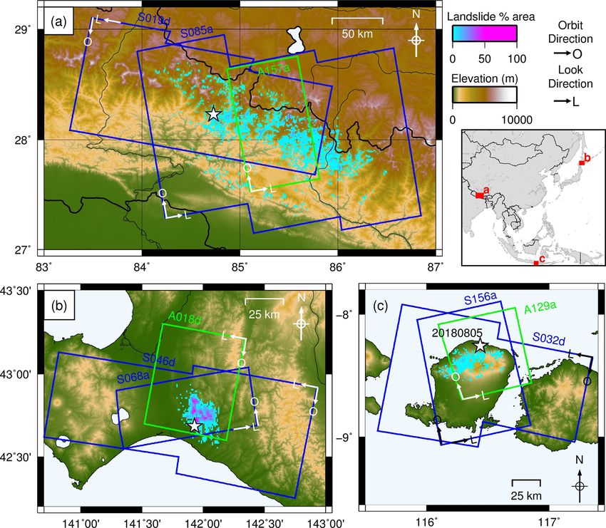
Figure 1. SAR coverage of the three case study regions: (a) the 2015 Gorkha, Nepal, earthquake; (b) the 2018 Hokkaido, Japan, earthquake;
and (c) the 2018 Lombok, Indonesia, earthquake. Sentinel-1 scenes shown in blue. ALOS-2 scenes shown in green. Landslide data from
Ferrario (2019), Roback et al. (2017) and Zhang et al. (2019). White stars show earthquake epicentres. White arrows show satellite orbit (O)
and look direction (L). Adapted from Burrows et al. (2020).
2 Data and methods inventory of Zhang et al. (2019) of 5265 landslides triggered
by the Mw 6.6 Hokkaido, Japan, earthquake; and the inven-
Empirical models of landslide hazard (represented here by tory of Ferrario (2019) of 4823 landslides triggered by the
LAD) adopt a functional form that is driven by a training Mw 6.8 Lombok, Indonesia, earthquake on 5 August 2018
dataset of mapped landslides rather than by the mechanics of (see Fig. 1 for the extent of triggered landslides from each of
slope stability. Since LAD is a continuous measure, our aim these earthquakes and the spatial and temporal coverage of
was to carry out a regression between a training dataset of the SAR data used here). The performance of five SAR-based
mapped LAD and a selection of input features (e.g. slope, el- methods using the same SAR data used here has already been
evation, land cover) that influence landslide likelihood. The carried out for these three case study earthquakes (Burrows
resultant function can then be used to predict LAD in areas et al., 2020). This allows a direct comparison between the
where there are no mapped landslide data available based performance of the models developed in this study and that
on these input features. In this section, we first describe the of existing SAR-based methods of landslide detection. Pre-
landslide data used to train and test our models. Second, we dicted LAD based on the empirical model of Nowicki Jessee
describe the different input features which we used in the et al. (2018) was also available to download for these three
regression to predict LAD. Third we describe the random events from the USGS website.
forests method and its implementation in this study. Finally We converted the three polygon landslide inventories to
we describe the metrics used to assess model performance. rasters with a cell size of 20×22 m. We then calculated LAD
within 10×10 squares of these 20×22 m cells, resulting in an
2.1 Landslide datasets aggregate landslide surface with a resolution of 200 × 220 m.
This is the same as the resolution at which Burrows et al.
We used polygon landslide inventories compiled for three (2020) assessed SAR-based methods of landslide detection,
large earthquakes that each triggered thousands of landslides: allowing a direct comparison with that study, and similar to
the inventory of Roback et al. (2017) of 24 915 landslides the resolution of the model of Nowicki Jessee et al. (2018),
triggered by the Mw 7.8 2015 Gorkha, Nepal, earthquake; the
https://doi.org/10.5194/nhess-21-2993-2021 Nat. Hazards Earth Syst. Sci., 21, 2993–3014, 2021
2996                 K. Burrows et al.: Integrating empirical models and satellite radar can improve landslide detection

whose products are provided at a resolution of 0.002◦ (ap-        graphic input features, it was possible to predict the spatial
proximately 220 m, depending on latitude).                        distribution of landslides triggered by the Hokkaido earth-
                                                                  quake using a model trained on landslides triggered by a
2.2    Training and test datasets                                 heavy rainfall event in Kyushu, 2017, but that it was not
                                                                  possible to predict landslides triggered by the Kyushu event
When developing an empirical model, it is necessary to di-        using a model trained on Hokkaido. Therefore, given the
vide the data into two parts: a training dataset, which is used   small number of case studies used here to train our prelimi-
to train the random forest; and a test dataset, which is used     nary global model, we expect a similar performance to that
to test model performance. Here we used two types of model        observed by Ohki et al. (2020); i.e. we do not expect high
setup: same-event models trained on a small mapped area of        performance on all predicted events. Instead, a high perfor-
an event to predict the landslide distribution across the rest    mance on at least one predicted event would suggest that
of the affected area (e.g. Robinson et al., 2017) and global      our approach is worthy of further investigation and is likely
models trained on historic landslide inventories to predict a     to improve when trained on a number of case studies more
new event (e.g. Kritikos et al., 2015; Nowicki et al., 2014;      comparable to those used by current gold-standard models
Nowicki Jessee et al., 2018; Tanyas et al., 2019).                (i.e. 23–25).
   The real-world application of a same-event model is that
a small number of landslides can be mapped manually from          2.3     Input features
optical satellite imagery in the days following the earthquake.
Provided these landslides are dispersed across the study area     A large number of possible input features have been used in
to constitute a representative training dataset, their distri-    previous work on landslide susceptibility mapping, includ-
bution can then be used to predict the landslide distribu-        ing a wide range of topographic parameters, ground shaking
tion across the whole affected area in much less time than        estimates, rainfall data, lithology, land cover, and distance to
would be required to manually map the whole area (Robin-          features such as rivers, roads and faults. Here we limited the
son et al., 2017). For our same-event model, we randomly          model input features to globally available datasets in order
selected 250 landslide (LAD ≥ 0.01) and 250 non-landslide         to ensure the widest applicability of the results. We targeted
(LAD < 0.01) pixels for use as training data. Robinson et al.     our model at earthquake- rather than rainfall-triggered land-
(2017) demonstrated that 250 landslide samples were suffi-        slides, as these have been more widely used as case studies
cient to train their landslide probability model. Since here we   when developing and testing SAR-based methods of land-
use 200 × 220 m pixels, 250 pixels is equivalent to a mapped      slide detection (e.g. Aimaiti et al., 2019; Burrows et al., 2019;
area of around 11 km2 .                                           Jung and Yun, 2019; Yun et al., 2015), and detailed poly-
   For the second approach, in which an empirical model           gon inventories of thousands of landslides triggered by a sin-
is trained on a global inventory of past landslides, we           gle earthquake (Ferrario, 2019; Roback et al., 2017; Zhang
trained the random forest on two of our case study events         et al., 2019) provide a good source of test and training data
and predicted the third. In this case, we randomly se-            for the model. In this section, we describe the topographic,
lected 1000 landslide (LAD ≥ 0.01) and 1000 non-landslide         ground shaking, land cover and lithology input features used
(LAD < 0.01) pixels from each event. The resulting model          to generate the initial same-event models. We also describe
was therefore trained on equal numbers of pixels from the         the model of Nowicki Jessee et al. (2018), which we used as
two training events, which prevents it from being domi-           a base for the global models, and the SAR-based input fea-
nated by the larger training event. We trained an ensemble        tures that we added to the same-event and global models. A
of 100 models, performing the random undersampling inde-          summary of these inputs and which of our models they are
pendently each time so that each model within the ensemble        used in is given in Table 1.
is trained on a different set of cells. We then estimated LAD
using each model and took the median ensemble prediction          2.3.1    Topographic features
as our final model. This process allows the model to use more
of the available training data and improves robustness. It also   For input features derived from topography, we used the 30 m
allows calculation of upper and lower bounds for the LAD of       Shuttle Radar Topography Mission (SRTM) digital elevation
every cell, as well as other statistical parameters such as the   model (DEM) (Farr et al., 2007). When processing the SAR
variance in predicted LAD.                                        data, this DEM was resampled to a resolution of 20 m × 22 m
   It should be noted that successful global empirical land-      using linear interpolation. From this resampled DEM, we cal-
slide prediction models are trained on data from considerably     culated slope and aspect using a 3×3 moving window and the
more case study events than this; for example, the model used     compound topographic index (CTI), a static proxy for pore
by the USGS of Nowicki Jessee et al. (2018) was trained           water pressure, which alters the effective normal stress on the
on 23 landslide inventories, and the model of Tanyas et al.       failure surface and thus the material strength (Moore et al.,
(2019) was trained on 25. Ohki et al. (2020) demonstrated         1991). We aggregated 10 × 10 grids of these cells to produce
that when using fully polarimetric SAR data alongside topo-       input features at a 200 m × 220 m scale. For each aggregate

Nat. Hazards Earth Syst. Sci., 21, 2993–3014, 2021                                https://doi.org/10.5194/nhess-21-2993-2021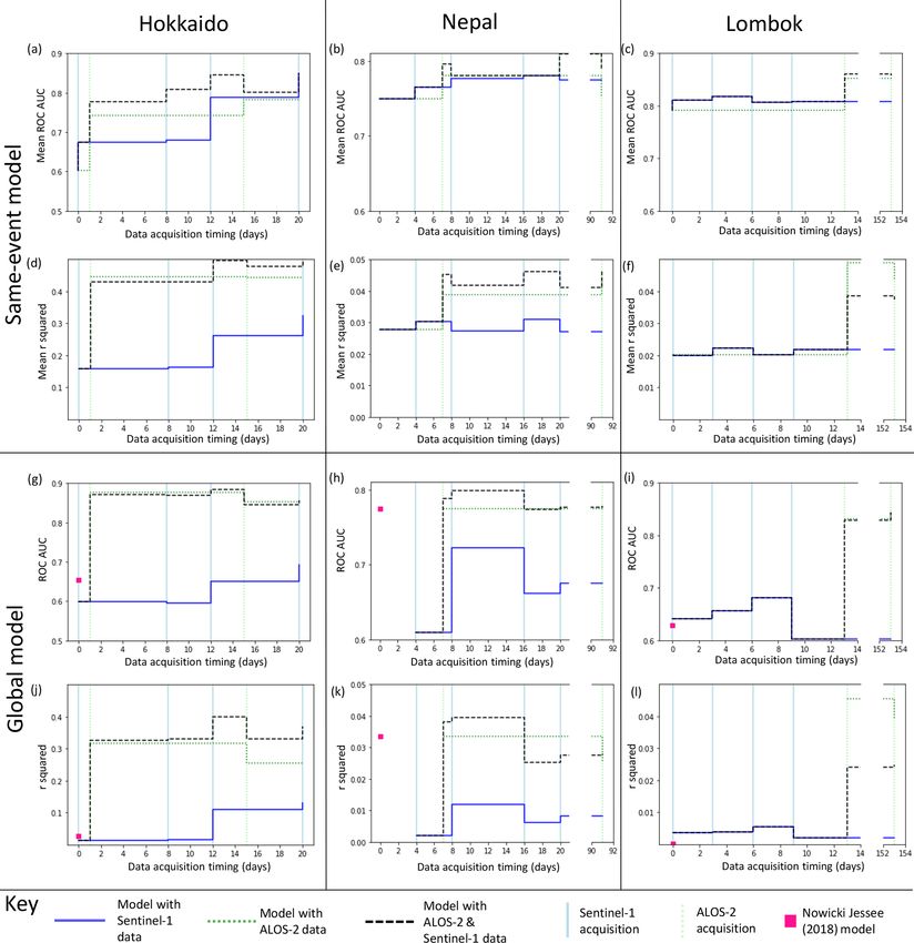
K. Burrows et al.: Integrating empirical models and satellite radar can improve landslide detection                                   2997

Table 1. Input features used in the random forest models and whether they were used in the same-event or global models. The table is divided
into conventional predictors of landslide likelihood and those based on InSAR coherence. For the latter, the case where only data from the
Sentinel-1 (S-1) satellite were used is noted; otherwise, both Sentinel-1 and ALOS-2 data were used.

                             Input feature                            Same-event models        Global models
                             Mean elevation                           X
                             Standard deviation of elevations         X
                             Maximum slope                            X
                             Mean slope                               X
                             Standard deviation of slopes             X
                             Circular mean of slope aspect            X
                             Mean compound topographic index          X
                             Relief                                   X
                             Peak ground velocity                     X
                             Lithology                                X
                             Land cover                               X
                             USGS ground failure product                                       X
                             Co-event coherence                       X                        X
                             Co-event coherence loss (CECL)           X                        X
                             Boxcar–sibling coherence (Bx–S)          X (S-1 only in Nepal)    X (S-1 only)
                             Post-event coherence                     X                        X (S-1 only)
                             Post-event coherence increase (PECI)     X                        X
                             Sum of CECL and PECI                     X                        X
                             Maximum CECL or PECI                     X                        X

200×220 m cell, we calculated the mean 20 m × 22 m cell el-               the 200 × 220 m geometry used here using a linear interpo-
evation (used by Catani et al., 2013; Nowicki et al., 2014), the          lation. The uncertainty of the ShakeMap product varies de-
standard deviation of cell elevations (used by Catani et al.,             pending on the local seismic network used to gather the shak-
2013), the maximum slope within an aggregate cell (used                   ing data on which the shaking estimates are based (Worden
by Nowicki et al., 2014), the mean slope within an aggre-                 et al., 2020) but is not currently taken into account when
gate cell (used by Nowicki Jessee et al., 2018; Robinson                  using these estimates in empirical models (Nowicki Jessee
et al., 2017; Kritikos et al., 2015; Tanyas et al., 2019), the            et al., 2018).
standard deviation of pixel slopes within an aggregate cell                  An initial estimate of ground shaking is generally available
(used by Catani et al., 2013; Tanyas et al., 2019), the circu-            within hours of an earthquake from the USGS ShakeMap
lar mean of the aspect (used by Chen et al., 2017), the mean              web page and is then refined as more data become avail-
compound topographic index (used by Nowicki Jessee et al.,                able. The difference that these updates to the ground shaking
2018; Tanyas et al., 2019), and the relief or maximum ele-                estimates can make to empirical models of landsliding has
vation difference between all 20 m × 22 m pixels within the               been explored by Allstadt et al. (2018) and Thompson et al.
aggregate cell (used by Tanyas et al., 2019).                             (2020). Here our aim was to investigate changes to modelled
                                                                          landsliding due to the incorporation of SAR data, and so for
2.3.2   Ground shaking estimates                                          simplicity we chose to keep all other input features constant
                                                                          through time. We used the final version of PGV published for
                                                                          each event in all our models. In reality, model performance
The inclusion of ground shaking information is what differ-
                                                                          would evolve both due to updates to the estimated PGV and
entiates an earthquake-specific prediction of triggered land-
                                                                          the availability of SAR data, but SAR data are also used to
sliding (used here) from a static estimate of landslide sus-
                                                                          improve PGV estimates, and the final “best” PGV estimate is
ceptibility (e.g. Nadim et al., 2006). Past studies have used
                                                                          often achieved when the first post-event SAR data are incor-
Modified Mercalli Intensity (Kritikos et al., 2015; Tanyas
                                                                          porated. Therefore, in practice, SAR-based landslide indica-
et al., 2019), peak ground acceleration (Robinson et al., 2018;
                                                                          tors will only be added to final or close-to-final versions of
Nowicki et al., 2014; Tanyas et al., 2019) and peak ground
                                                                          these empirical models.
velocity (PGV) (Nowicki Jessee et al., 2018; Tanyas et al.,
2019). Here, we used PGV, as this does not saturate at high
shaking intensities (Nowicki Jessee et al., 2018). Gridded
PGV estimates are available with pixel spacing 0.00083◦ as
part of the USGS ShakeMap product. We resampled this onto

https://doi.org/10.5194/nhess-21-2993-2021                                       Nat. Hazards Earth Syst. Sci., 21, 2993–3014, 2021
2998                 K. Burrows et al.: Integrating empirical models and satellite radar can improve landslide detection

2.3.3   Lithology                                                 and no skill in Lombok or Nepal, which is not representa-
                                                                  tive of the performance of existing global models (e.g. Now-
Lithology is one factor that determines rock strength, and        icki Jessee et al., 2018; Tanyas et al., 2019). This poor per-
therefore landslide likelihood (Nadim et al., 2006), and has      formance is likely to be due to the limited number of case
been used in several empirical landslide susceptibility mod-      studies used as training data in our global models and would
els (Chen et al., 2017; Kirschbaum and Stanley, 2018; Now-        make it difficult to draw conclusions on the benefits of adding
icki Jessee et al., 2018). We used the Global Lithologi-          SAR to a global empirical model. We found that by replacing
cal Map database (GLiM) (Hartmann and Moosdorf, 2012),            the individual input features with the model output of Now-
which has 13 basic lithological classes, with additional “wa-     icki Jessee et al. (2018), we improved model performance
ter bodies”, “ice and glacier” and “no data” classes, which       in Nepal and Lombok and obtained a more consistent result
are supplied as polygon data. These data are provided in          across the three events.
vector format. We rasterised these data onto the 20 × 22 m           The models of Nowicki Jessee et al. (2018) are published
grid at which the SAR data were processed. Then for each          within hours following a large earthquake for use in haz-
200 × 220 m aggregate pixel, we took the dominant basic           ard assessment and emergency response coordination and are
lithological class (i.e. that with the largest area share), re-   available from the USGS website. They are generated using
sulting in a categorical input feature. Random forests can        logistic regression based on PGV, slope, CTI, lithology and
accept both continuous and categorical input features, but        land cover data (Nowicki Jessee et al., 2018). As described
empty categories in the training data can lead to biases in       in Sect. 2.3.2, USGS estimates of PGV are updated multiple
the model (Au, 2018). To avoid this, we used the “one-hot”        times after an earthquake, and the ground failure products
method, in which each category is supplied to the model as        based on these are also updated. Again, we use final pub-
a separate dummy input feature, i.e. a binary surface of, for     lished version of the ground failure product (based on the
example, “unconsolidated sediment” and “everything else”          final PGV estimates) in all our models. However, any conclu-
(Au, 2018). The number of input feature maps used for each        sions drawn here about the advantage of incorporating SAR
model was equivalent to the number of lithological categories     into the model should remain valid for earlier versions of the
present in each case: six in Hokkaido, nine in Nepal and six      ground failure product. The models of Nowicki Jessee et al.
in Lombok.                                                        (2018) are published at a similar spatial resolution (around
                                                                  0.002◦ ) to our models. Therefore, the only processing step
2.3.4   Land cover                                                required was to resample them onto the geometry of our other
                                                                  input data (200 × 220 m pixels).
Nowicki Jessee et al. (2018) used land cover as a proxy for
vegetation coverage and type, as the composition of the soil      2.3.6   InSAR coherence features (ICFs)
and the presence or absence of plant roots can affect slope
stability. Here we used land cover data downloaded from the       Multiple studies have demonstrated that methods based on
European Space Agency (ESA) Climate Change Initiative,            InSAR coherence can be used in landslide detection (e.g.
which includes yearly maps of 22 land cover categories com-       Aimaiti et al., 2019; Burrows et al., 2019, 2020; Jung and
piled at a 300 m resolution from 1992–2015 (ESA, 2017).           Yun, 2019; Yun et al., 2015). An interferogram is formed
We used the 2014 map as the most recent land cover map            from two SAR images acquired over the same area at differ-
preceding all of our case study events. Like lithology, land      ent times, and its coherence is sensitive to a number of fac-
cover is a categorical variable; thus, we used the same one-      tors including changes to scatterers between the two image
hot method described in Sect. 2.3.3 to avoid biasing due to       acquisitions and, particularly in areas of steep topography,
empty categories and selected the dominant land cover type        changes to the image acquisition geometry (Zebker and Vil-
within each 200 m × 220 m aggregate cell. As for lithology,       lasenor, 1992). Changes in soil moisture (Scott et al., 2017);
the number of land cover input feature maps used for each         movement of vegetation due to wind (Tanase et al., 2010);
case study area was equivalent to the number of categories        growth, damage or removal of vegetation (Fransson et al.,
present: 15 in Hokkaido, 16 in Nepal and 16 in Lombok.            2010); and damage to buildings (Fielding et al., 2005; Yun
                                                                  et al., 2015) are all examples of processes which can alter the
2.3.5   USGS ground failure product                               scattering properties of the Earth’s surface and so lower the
                                                                  coherence of an interferogram. InSAR coherence is a mea-
For our global model, instead of the set of individual input      sure of the signal-to-noise ratio of an interferogram estimated
feature maps described above, we use one single feature map       on a pixel-by-pixel basis from the similarity in amplitude and
that encapsulates the likely best results from a global model     phase change of small numbers of pixels (Just and Bamler,
trained across a large number of events: the output USGS          1994).
Ground Failure product of Nowicki Jessee et al. (2018). This         We used single-polarisation SAR data from two SAR sys-
was necessary since we found that models generated from           tems in this study: the C-band Sentinel-1 SAR satellite op-
individual input feature maps had limited skill in Hokkaido       erated by ESA and the Phased Array type L-band SAR-

Nat. Hazards Earth Syst. Sci., 21, 2993–3014, 2021                               https://doi.org/10.5194/nhess-21-2993-2021
K. Burrows et al.: Integrating empirical models and satellite radar can improve landslide detection                          2999

2 (PALSAR-2) sensor on the Advanced Land Observation               The post-event ALOS-2 coherence was therefore omitted
Satellite 2 (ALOS-2) operated by the Japan Aerospace Ex-           from our global models.
ploration Agency (JAXA). For each case study earthquake,              As well as the raw coherence surfaces, we used the five
we used ascending- and descending-track Sentinel-1 SAR             coherence-based methods tested by Burrows et al. (2020)
imagery and a single track of ALOS-2 PALSAR-2 imagery              as input features, all of which showed some level of land-
(Fig. 1). This volume of SAR data is available in the immedi-      slide detection skill in that study. The output of each of these
ate aftermath of the majority of earthquakes (Burrows et al.,      methods is a continuous surface that can be interpreted as
2020). These two satellite systems acquire SAR data at dif-        a proxy for landslide intensity. First, the co-event coher-
ferent wavelengths and so interact slightly differently with       ence loss (CECL) method uses the decrease in coherence
the ground surface, with ALOS-2 generally being less noisy         between a pre-event and co-event interferogram to identify
in heavily vegetated areas than Sentinel-1 (Zebker and Vil-        “damaged” pixels (Fielding et al., 2005; Yun et al., 2015).
lasenor, 1992). SAR data are acquired obliquely, which in ar-      The boxcar–sibling (Bx–S) method of Burrows et al. (2019)
eas of steep topography can lead to some slopes being poorly       uses the difference between two different co-event coherence
imaged by the SAR sensor. Here all data were acquired at an        estimates to remove large-spatial-scale coherence variations
angle of 31.4–43.8◦ to vertical. Descending-track data were        from the landslide detection surface. Finally three methods
acquired with the satellite moving south and looking west,         presented by Burrows et al. (2020) incorporate the coherence
while ascending-track data were acquired with the satellite        of a post-event interferogram to detect landslides, making
moving north and looking east. Therefore, slopes which are         use of the fact that the coherence decrease caused by a land-
poorly imaged in ascending data are likely to be better im-        slide is temporary. The post-event coherence increase (PECI)
aged by the descending track and vice versa. It is for this        method uses the difference between the post-event and co-
reason that we employed two tracks of Sentinel-1 data, but         event coherences. The PECI and CECL methods are then
this is currently not often available for L-band SAR. We pro-      combined in two further methods: the sum of the co-event co-
cessed the SAR data using GAMMA software, with Sentinel-           herence loss and post-event coherence increase (1C_sum);
1 data processed using the LiCSAR package (Lazeckỳ et al.,        and the maximum coherence change (1C_max), where for
2020). The data were processed in a range × azimuth coor-          every pixel, whichever is largest of PECI or CECL is taken.
dinate system and then projected into a geographic coordi-            The majority of the methods outlined in this section use
nate system with a spatial resolution of 20 m × 22 m. Further      a “boxcar” coherence estimate, using pixels from within a
details on the spatial and temporal resolution of these SAR        3 × 3 window surrounding the target pixel in the coherence
data, on their processing and on parameter choices made            estimation. The only exception to this is the Bx–S method,
in the generation of the CECL, Bx–S, PECI, 1C_sum and              which also uses a “sibling” coherence estimate in which an
1C_max surfaces can be found in Burrows et al. (2020).             ensemble of pixels is selected from within a wider window
   We aimed to combine InSAR coherence methods with em-            for coherence estimation using the RapidSAR algorithm of
pirical models. To achieve this, we used multiple InSAR            Spaans and Hooper (2016) (Burrows et al., 2019). This sib-
coherence methods as input features. The first coherence           ling coherence estimation requires additional data (a mini-
method we used was the coherence of the co-event interfer-         mum of six pre-seismic images), and so it was not possible
ogram (formed from two images spanning the earthquake).            to calculate this using ALOS-2 data for the 2015 Nepal earth-
The movement of material and removal of vegetation by a            quake, as this event occurred very early in the lifetime of the
landslide alters the scattering properties of the Earth’s sur-     satellite. The Bx–S method with ALOS-2 data was therefore
face, resulting in low coherence. This gives landslides a low      not used in Nepal or in any of the global models we tested.
coherence in a co-event interferogram. Burrows et al. (2019)
and Vajedian et al. (2018) demonstrated that this had some         2.4   Random forest theory and implementation
potential in triggered landslide detection. Second, we used
the coherence of the post-event interferogram (formed from         Random forests are an extension of the decision tree method,
two images acquired after the earthquake). Coherence is de-        a supervised machine learning technique in which a sequence
pendent on the land cover, with vegetated areas generally          of questions are applied to a dataset in order to predict some
having a lower coherence than bare rock or soil (Tanase et al.,    unknown property, for example to predict landslide suscep-
2010). Therefore, the bare rock or soil exposed following a        tibility based on features of the landscape (e.g. Chen et al.,
landslide is likely to have a higher coherence than the sur-       2017). A random forest comprises a large number of decision
rounding vegetation. This input feature was found to be ben-       trees, each seeing different combinations of input data, which
eficial in most cases, but the distribution of post-event coher-   then make a combined prediction. This avoids overfitting the
ence values varied significantly between events when using         training data, a problem when using individual decision trees
ALOS-2 data. This may be because the wait time between the         (Breiman, 2001). First the training dataset is bootstrapped so
first and second post-event images varied significantly be-        that each tree sees only a subset of the original pixels. Each
tween the events (from 14 to 154 d, Burrows et al., 2020).         tree carries out a series of “splits”, in which the data are di-
                                                                   vided in two based on the value of an input feature. These

https://doi.org/10.5194/nhess-21-2993-2021                                Nat. Hazards Earth Syst. Sci., 21, 2993–3014, 2021
3000 K. Burrows et al.: Integrating empirical models and satellite radar can improve landslide detection
Table 2. Hyperparameter options for the random forest in scikit-learn over which a grid search optimisation was carried out (Pedregosa et al.,
2011).
Hyperparameter Definition GridSearch
n_estimators The number of decision trees that make up a forest [75, 100, 125]
max_features The number of input features (as a function of the total) considered when looking for a split [“log2”, “sqrt”]
max_depth The maximum depth of the tree [10, 15, 20, 30]
min_samples_split The minimum number of samples at a node for a split to be allowed [2, 3, 4, 5]
min_samples_leaf The minimum number of samples that would result at each leaf for a split to be allowed [2, 10]
splits are chosen based on the improvement they offer to the result in a more computationally expensive model. Second,
ability of each tree to correctly predict its training data. Every max_features defines the fraction of possible input features
tree remembers how it split the training data and then applies considered when selecting how the split of the data is calcu-
the same splits as it attempts to model the test data. For ran- lated. For example, our initial same-event models had 11 in-
dom forest regression, the mean value of all trees is taken put features (Table 1), so with square root (sqrt) √ selected,
as the model output for every sample (Breiman, 2001). To the model will assess possible splits based on 11 ≈ 3 in-
aid understanding, we include a simple example of random put features before identifying the best split. The “depth” of
forest regression in the Supplement. each decision tree describes the number of times the data
Here, we used random forests to carry out the regression will be split if it takes the longest path from the begin-
between the input features described in Sect. 2.3 and LAD. ning of the tree to the end. This is limited by Max_depth,
Random forests are well suited to the combination of SAR which defines the maximum depth of each decision tree. Fi-
methods with static landslide predictors for several reasons. nally, min_samples_split is the minimum number of samples
Random forests are relatively computationally inexpensive a node has to contain before splitting for a split to be allowed,
and, because of this, can use a large number of input features. while min_samples_leaf is the minimum number of samples
Random forests do not require input features to be indepen- assigned to either branch after splitting for a split to be al-
dent, which is advantageous here since InSAR coherence is lowed. For each of these five hyperparameters, we selected
sensitive to both slope and land cover, as well as the presence several possible options, which are shown in the final col-
or absence of landslides. Input features of random forests do umn of Table 2. We then used the GridSearchCV function in
not need to be monotonic and can be categoric or continuous. sci-kit learn to select an optimised model. This function ran
Catani et al. (2013), Chen et al. (2017), Fan et al. (2020) and models with every possible combination of these values, us-
Ohki et al. (2020) have demonstrated that random forests can ing 4-fold cross-validation over our training data to identify
yield good results in landslide prediction. the optimal hyperparameter combination (Pedregosa et al.,
To implement the random forests method, we used the 2011).
Python scikit-learn package (Pedregosa et al., 2011). The
model is defined by a number of hyperparameters that can 2.4.1 Feature importances
have a noticeable effect on the model. The first of these is
the criteria on which a split should be assessed. In our mod- The importance of each input feature was calculated from
els, splits were carried out that minimised the mean absolute the decrease in MAE resulting from splits on that feature for
error (MAE). This criterion was selected based on Ziegler each tree and then averaged over all the trees to obtain fea-
and König (2014). The second hyperparameter describes the ture importance at the forest level. This calculation gives an
bootstrapping step. Here the data were bootstrapped so that a indication of how reliant the model is on each feature, with
number of random samples was taken equal to the number of the sum of importances across all input features equal to one
pixels in the training dataset. Each individual pixel is there- (Liaw and Wiener, 2002). Feature importance therefore helps
fore likely to appear at least once in around two-thirds of with interpreting the model and can allow unimportant fea-
the bootstrapped datasets (Efron and Tibshirani, 1997). This tures to be eliminated from future models, reducing compu-
process improves the stability of the model by ensuring that tation time (e.g. Catani et al., 2013; Díaz-Uriarte and De An-
each tree is trained on a slightly different subset of the train- dres, 2006). However, it should be noted that the importance
ing data (Breiman, 2001). of categorical input features (here lithology and land cover) is
Table 2 shows a further five hyperparameters that define often underestimated, since in this case the number of possi-
the setup of a random forest model in scikit-learn (Pedregosa ble splits is limited to the number of categories present in the
et al., 2011). First the number of trees, n_estimators, defines training data. Furthermore, since our input features are not
the number of decision trees that make up a forest. More independent (for example, InSAR coherence can be affected
trees can increase model accuracy up to a point but also by land cover and slope), caution should be taken when draw-
ing conclusions from importance values.
Nat. Hazards Earth Syst. Sci., 21, 2993–3014, 2021 https://doi.org/10.5194/nhess-21-2993-2021K. Burrows et al.: Integrating empirical models and satellite radar can improve landslide detection 3001
2.5 Performance metrics 3 Results
Each model generated a raster of continuous predictor vari- 3.1 Same-event models
ables, corresponding to the modelled LAD in the range [0, 1].
We assessed model performance by comparing the test areas Figure 2 shows the effect on model AUC (Fig. 2a–c) and r 2
of these predicted surfaces with the mapped LAD calculated (Fig. 2d–f) of adding Sentinel-1 and ALOS-2 data to a land-
from the inventories of Ferrario (2019), Roback et al. (2017) slide susceptibility model trained on 250 landslide and non-
and Zhang et al. (2019) in Sect. 2.1. We used two metrics in landslide pixels mapped following an event and tested on the
assessing model performance: ROC analysis and the coeffi- remaining pixels. Since the model performance varied de-
cient of determination (r 2 ). pending on which 500 pixels were used as training data, we
ROC analysis has been widely used in studies of land- ran each model 30 times and give the mean AUC and r 2 of
slide prediction and detection and is relatively simple to in- these models in Fig. 2a–f.
terpret (e.g. Burrows et al., 2020; Robinson et al., 2017; The initial models for Hokkaido, Nepal and Lombok had
Tanyas et al., 2019). Additionally, the use of ROC analysis AUC values of 0.60, 0.75 and 0.79 and r 2 values of 0.17,
allows comparison between the models in this study and the 0.027 and 0.020 respectively. We observed this combination
InSAR-coherence-based methods of Burrows et al. (2020). of comparatively high ROC AUC values and very low r 2 val-
ROC analysis requires a binary landslide surface for vali- ues for all of the models tested in this paper as well as for the
dation, so we applied a threshold to the mapped LAD sur- models of Nowicki Jessee et al. (2018). These low r 2 values
face calculated in Sect. 2.1, assigning aggregate cells with have implications for how the current generation of empiri-
LAD > 0.1 as “landslide” and < 0.1 as “non-landslide”. Set- cal models should be interpreted, and we discuss this further
ting this threshold higher would test the model’s ability to in Sect. 4.1.
detect more severely affected pixels, while setting it lower In almost all cases, incorporating ICFs improved model
would test the model’s ability to more completely capture performance in terms of AUC, with the biggest improvement
the extent of the landsliding. We chose 0.1 to strike a bal- observed when ICFs from the first ALOS-2 image are added.
ance between these two factors. These aggregate cells with The addition of these first ALOS-2 ICFs also results in an
LAD > 0.1 contain 77 % of the total area of the individual increase in r 2 for each case study region. The biggest im-
landslide polygons in Nepal, 94 % in Hokkaido and 46 % in provement is seen in Hokkaido, where the addition of these
Lombok. Using this binary aggregate landslide surface, the ALOS-2 ICFs results in a increase in r 2 from 0.17 to 0.45
false positive rate (the fraction of mapped non-landslide pix- and an increase in AUC from 0.68 to 0.78. Although these
els wrongly assigned as landslide by the model) and true ALOS-2 ICFs result in the largest improvement in model per-
positive rate (the fraction of mapped landslide pixels cor- formance, in all three events the model incorporating both
rectly assigned as landslide by the model) were calculated ALOS-2 and Sentinel-1 ICFs outperforms the model using
at a range of thresholds and plotted against each other to pro- ALOS-2 ICFs alone in terms of AUC. In terms of r 2 , the
duce a curve. The area under this curve (AUC) then indicates combined model outperforms the ALOS-2 only model in
the predictive skill of the model, with a value of 0.5 indicat- Nepal, but the ALOS-2 only model performs best in Lom-
ing no skill and 1.0 indicating a perfect model (Hanley and bok. In Hokkaido, the combined model performs best after
McNeil, 1982). The ROC AUC values calculated here there- the third Sentinel-1 acquisition. Sentinel-1 data are also often
fore represent the ability of the model to identify pixels with available sooner after a triggering earthquake than ALOS-2
LAD > 0.1. data, due to the short revisit time of the Sentinel-1 satellites.
The second method we used to assess model performance
was to carry out a linear regression between the observed and 3.2 Global models
predicted LAD. The r 2 of this regression is calculated as the
fraction of the variability in predicted LAD that is explained An alternative to training on a small part of the affected area
by this linear model. A high r 2 coefficient value (up to a max- is to train the model on inventories from past earthquakes.
imum of 1.0) indicates low levels of random errors, while an To test the effect that incorporating ICFs might have on such
r 2 close to zero indicates that levels of random errors in the models using our three case studies, we applied a leave-one-
model are too high to obtain a good fit to observed LAD. out cross-validation approach: we tested predictions of LAD
Therefore, r 2 indicates the ability of our random forest mod- for each earthquake that were generated using models trained
els to avoid random errors in their prediction of LAD, while on the other two earthquakes. Figure 2 shows the effect on
the ROC AUC indicates their ability to identify severely af- model AUC (Fig. 2g–i) and r 2 (Fig. 2 j–l) of adding ALOS-2
fected pixels. and Sentinel-1 ICFs to the input features used in training the
model.
The USGS landslide model of Nowicki Jessee et al. (2018)
had AUC values of 0.65 in Hokkaido, 0.62 in Lombok and
0.77 in Nepal and r 2 of 0.026, 0.033 and 0.0022 respec-
https://doi.org/10.5194/nhess-21-2993-2021 Nat. Hazards Earth Syst. Sci., 21, 2993–3014, 20213002 K. Burrows et al.: Integrating empirical models and satellite radar can improve landslide detection Figure 2. Step plots showing the change in ROC AUC (a–c, g–i) and r 2 (d–f, j–l) for each of the three events. Models in panels (a)–(f) were trained on a small part of each study area, while in panels (g)–(l) landslide areal density was predicted using a model trained on the other two case study regions in each case. tively. In order to test the effect of adding ICFs to a global acquired within 2 weeks of each earthquake results in better model, we used the USGS model as an input feature along- and more consistent model performance. This improvement side the ICFs listed in Sect. 2.3. As with the same-event can be observed in Fig. 4, which shows the models of Now- models (Sect. 3.1), incorporating ICFs improved model per- icki Jessee et al. (2018) alongside those incorporating SAR formance in almost all cases, with the largest improvement data acquired within 2 weeks of each earthquake. in terms of both AUC and r 2 seen with the addition of the first ALOS-2 ICFs. In all three cases, our global models at 2 weeks have an AUC > 0.8 and outperform the USGS land- slide model of Nowicki Jessee et al. (2018) in terms of AUC and r 2 . Overall, the addition of ICFs derived from SAR data Nat. Hazards Earth Syst. Sci., 21, 2993–3014, 2021 https://doi.org/10.5194/nhess-21-2993-2021
K. Burrows et al.: Integrating empirical models and satellite radar can improve landslide detection                                    3003

Figure 3. Timelines of modelled landslide areal density for each event, starting with no SAR data (a, d, g). Panels (b), (e) and (h) show the
model using SAR data acquired within 2 weeks of the earthquake, and panels (c), (f) and (i) show landslide areal density calculated from
polygon inventories for each event (Ferrario, 2019; Roback et al., 2017; Zhang et al., 2019). The mapping extent of each of these inventories
is shown by a black polygon. White polygons in the final row show areas unmapped by Roback et al. (2017) due to cloud cover in optical
imagery.

3.3   Do these models outperform individual InSAR                        InSAR coherence methods for landslide detection. AUC val-
      coherence methods?                                                 ues have been calculated here at the same resolution and with
                                                                         the same definition of a landslide or non-landslide aggregate
To assess whether a combined model of ICFs and landslide                 cell. This allows direct comparison between the performance
susceptibility is useful, it is necessary to compare it to the in-       of the models applied here and the InSAR coherence meth-
formation that could be obtained from SAR alone. The SAR                 ods alone. To assess the value added to the InSAR coher-
data and case studies used here are the same as those used               ence methods by the static landslide predictors (e.g. slope),
by Burrows et al. (2020) in their systematic assessment of               we also applied the random forest technique using the ICFs

https://doi.org/10.5194/nhess-21-2993-2021                                      Nat. Hazards Earth Syst. Sci., 21, 2993–3014, 2021
3004 K. Burrows et al.: Integrating empirical models and satellite radar can improve landslide detection
described in Sect. 2.3.6 as the only input features. Figure 5 study, topography was initially the most important input fea-
shows AUC values for (1) the combined model, (2) a SAR- ture but its importance gradually decreased as more SAR
only model and (3) the InSAR-coherence-based method rec- data were added, particularly in Hokkaido, where it ceased
ommended for each SAR image acquisition by Burrows et al. to be the most important feature after the ICFs from the first
(2020, Supplement). ALOS-2 image were added to the model. In the final mod-
For the same-event models (Fig. 5a–c), the combined els, ALOS-2 ICFs were consistently more important than
model outperforms the SAR-only model in almost all cases, Sentinel-1, particularly in Hokkaido where these become the
and in the initial days following the earthquake, when only most important feature in the model.
Sentinel-1 is available, the combined model outperforms the
coherence methods. This is particularly noticeable for Lom-
bok, as four Sentinel-1 images were acquired before the first 4 Discussion
ALOS-2 image following this event, and the model has a
consistently higher AUC than the individual Sentinel-1 co- We have presented the results of adding ICFs to two types of
herence surfaces (approximately 0.8 compared to 0.6). When landslide model: a same-event model trained on a small area
the coherence methods recommended by Burrows et al. of each case study earthquake and a global model, which is
(2020) are employed using ALOS-2 data, they outperform trained on two earthquakes to predict the third. In both cases,
both the combined and SAR-only models in terms of AUC we have demonstrated that model performance was signifi-
in two cases (the first ALOS-2 image after Hokkaido and the cantly improved by the addition of ICFs derived from data
second after Nepal) and perform similarly in the other four acquired within 2 weeks of an earthquake. In this section, we
cases. discuss some of the factors that could affect the applicability
For the global models, the difference between the SAR- of these models in an emergency response situation.
only and combined model is less pronounced, but in most
4.1 Model interpretation based on ROC AUC and r 2
cases, the combined model has a higher AUC than the SAR-
only model. Both models outperform the individual InSAR We have demonstrated that the addition of ICFs to empirical
coherence methods that use Sentinel-1 data in all cases ex- models of LAD based on topography, ground shaking esti-
cept the first Sentinel-1 image following the Nepal earth- mates, land cover and lithology significantly improves their
quake. The coherence methods of Burrows et al. (2020) out- performance in terms of ROC AUC and r 2 . However, while
perform both models when the second ALOS-2 image is the final AUC values are around 0.8 or higher, r 2 remains
available in Nepal and Lombok but have a similar perfor- below 0.05 in Nepal and Lombok. We also observed this
mance in the other cases. combination of relatively high AUC (0.63–0.77) alongside
We are also able to make a visual comparison between the low r 2 (0.0002–0.03) for the models of Nowicki Jessee et al.
InSAR coherence products of Burrows et al. (2020) and the (2018), which are published on the USGS website. This re-
2-week models shown here in Figs. 3 and 4. Burrows et al. sult directly impacts how the current generation of empir-
(2020) observed false positives south of the landslides trig- ical models at this spatial scale should be interpreted: the
gered by the Hokkaido earthquake, which they attribute to low r 2 values we have observed indicate that the ability of
wind damage to vegetation associated with Typhoon Jebi. the models to predict LAD as a continuous variable is poor,
They also observed false positives in built-up areas close to while the more encouraging AUC values indicate that the
the coast in Lombok. These areas of false positives are visi- models are well suited to discriminating between affected
bly dampened in both our same-event and our global 2-week and unaffected pixels. Therefore, in an emergency response
models. scenario, the model of Nowicki Jessee et al. (2018) and the
models presented here can be used to provide an estimate of
3.4 Feature importances the spatial extent and distribution of the triggered landsliding
after an earthquake but should not be interpreted as a reliable
Figure 6 shows the relative importance of each input fea- estimate of LAD.
ture in a random forest model when the model is trained on
data from Hokkaido (Fig. 6a), Nepal (Fig. 6b) and Lombok 4.2 Selection of the training data for the same-event
(Fig. 6c). For simplicity, the parameters have been grouped model type
by the data required to create them. For example, the impor-
tance of “topography” in Fig. 6 was calculated as the sum The same-event case we have presented here uses 500 train-
of the importances of maximum slope, mean slope, standard ing data cells randomly selected from across the study area.
deviation of slope, elevation, standard deviation of elevation, The aim of this process is to reduce the area that is required
relief, CTI and aspect. As described in Sect. 2.4.1, these mea- to be manually mapped from optical satellite data or field in-
sures of importance are limited since our input features are vestigations before an estimate of LAD can be generated over
not fully independent, but it is clear that the importance of the whole affected area and therefore to reduce the time taken
the ICFs increases through time in each case. For each case to generate a complete overview of the landsliding. An alter-
Nat. Hazards Earth Syst. Sci., 21, 2993–3014, 2021 https://doi.org/10.5194/nhess-21-2993-2021K. Burrows et al.: Integrating empirical models and satellite radar can improve landslide detection 3005 Figure 4. Timelines of modelled landslide areal density for each event. Panels (a), (d) and (g) show the results of the model of Nowicki Jessee et al. (2018) for each event. Panels (b), (e) and (h) show the model using SAR data acquired within 2 weeks of the earthquake, and panels (c), (f) and (i) show landslide areal density calculated from polygon inventories for each event (Ferrario, 2019; Roback et al., 2017; Zhang et al., 2019). The mapping extent of each of these inventories is shown by a black polygon. White polygons in the final row show areas not mapped by Roback et al. (2017) due to cloud cover in optical imagery. native scenario would be the case where cloud cover prevents ing dataset comprising all of the data outside the test area manual landslide mapping in some parts of the affected area. (Fig. 7d), which contained 5210 cells with LAD > 1 % across Robinson et al. (2017) noted that this clustering had a detri- an area of 47 km2 , so that after balancing by undersampling mental effect on the performance of their same-event model. non-landslide cells (see Sect. 2.4), the training dataset com- To explore this, we tested the ability of a same-event model prised 10 420 cells. The model shown in Fig. 7e used only to predict LAD for a selected area using only training data the data west of the training area (6106 pixels after balancing from outside that area (Fig. 7). We chose to test this in Nepal, across an area 21 km2 ). From here, the longitudinal extent as this event covered the largest area. We began with a train- of the training data used was halved each time, resulting in https://doi.org/10.5194/nhess-21-2993-2021 Nat. Hazards Earth Syst. Sci., 21, 2993–3014, 2021
You can also read