BFM17 v1.0: a reduced biogeochemical flux model for upper-ocean biophysical simulations
←
→
Page content transcription
If your browser does not render page correctly, please read the page content below
Geosci. Model Dev., 14, 2419–2442, 2021
https://doi.org/10.5194/gmd-14-2419-2021
© Author(s) 2021. This work is distributed under
the Creative Commons Attribution 4.0 License.

BFM17 v1.0: a reduced biogeochemical flux model for upper-ocean
biophysical simulations
Katherine M. Smith1 , Skyler Kern1 , Peter E. Hamlington1 , Marco Zavatarelli2 , Nadia Pinardi2 , Emily F. Klee3 , and
Kyle E. Niemeyer3
1 PaulM. Rady Department of Mechanical Engineering, University of Colorado, Boulder, CO, USA
2 Department of Physics and Astronomy, University of Bologna, Bologna, Italy
3 School of Mechanical, Industrial, and Manufacturing Engineering, Oregon State University, Corvallis, OR, USA

Correspondence: Katherine M. Smith (kmsmith@lanl.gov)

Received: 9 May 2020 – Discussion started: 13 July 2020
Revised: 19 February 2021 – Accepted: 2 March 2021 – Published: 5 May 2021

Abstract. We present a newly developed upper-thermocline,         provides improved correlations between several model out-
open-ocean biogeochemical flux model that is complex and          put fields and observational data, indicating that reproduc-
flexible enough to capture open-ocean ecosystem dynamics          tion of in situ data can be achieved with a low number of
but reduced enough to incorporate into highly resolved nu-        variables, while maintaining the functional group approach.
merical simulations and parameter optimization studies with       Notable additions to BFM17 over similar complexity models
limited additional computational cost. The model, which           are the explicit tracking of dissolved oxygen, allowance for
is derived from the full 56-state-variable Biogeochemical         non-Redfield nutrient ratios, and both dissolved and partic-
Flux Model (BFM56; Vichi et al., 2007), follows a bio-            ulate organic matter, all within the functional group frame-
logical and chemical functional group approach and allows         work.
for the development of critical non-Redfield nutrient ratios.
Matter is expressed in units of carbon, nitrogen, and phos-
phate, following techniques used in more complex models.
To reduce the overall computational cost and to focus on          1   Introduction
upper-thermocline, open-ocean, and non-iron-limited or non-
silicate-limited conditions, the reduced model eliminates cer-    Biogeochemical (BGC) tracers and their interactions with
tain processes, such as benthic, silicate, and iron influences,   upper-ocean physical processes, from basin-scale circula-
and parameterizes others, such as the bacterial loop. The         tions to millimeter-scale turbulent dissipation, are critical for
model explicitly tracks 17 state variables, divided into phy-     understanding the role of the ocean in the global carbon cy-
toplankton, zooplankton, dissolved organic matter, particu-       cle. These interactions cause multi-scale spatial and tempo-
late organic matter, and nutrient groups. It is correspondingly   ral heterogeneity in tracer distributions (Strass, 1992; Yoder
called the Biogeochemical Flux Model 17 (BFM17). After            et al., 1992; McGillicuddy et al., 2001; Gower et al., 1980;
describing BFM17, we couple it with the one-dimensional           Denman and Abbott, 1994; Strutton et al., 2012; Clayton,
Princeton Ocean Model for validation using observational          2013; Abraham, 1998; Bees, 1998; Mahadevan and Archer,
data from the Sargasso Sea. The results agree closely with        2000; Mahadevan and Campbell, 2002; Levy and Klein,
observational data, giving correlations above 0.85, except for    2015; Powell and Okubo, 1994; Martin et al., 2002; Ma-
chlorophyll (0.63) and oxygen (0.37), as well as with corre-      hadevan, 2005; Tzella and Haynes, 2007) that can greatly
sponding results from BFM56, with correlations above 0.85,        affect carbon exchange rates between the atmosphere and
except for oxygen (0.56), including the ability to capture        interior ocean, net primary productivity, and carbon export
the subsurface chlorophyll maximum and bloom intensity.           (Lima et al., 2002; Schneider et al., 2008; Hauri et al., 2013;
In comparison to previous models of similar size, BFM17           Behrenfeld, 2014; Barton et al., 2015; Boyd et al., 2016).
                                                                  There are still significant gaps, however, in our understand-

Published by Copernicus Publications on behalf of the European Geosciences Union.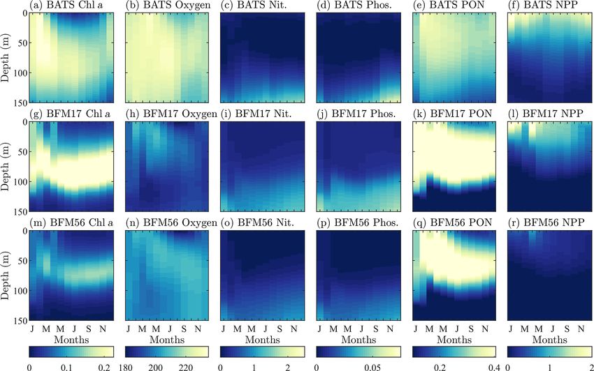
2420                                                               K. M. Smith et al.: A reduced biogeochemical flux model

ing of how these biophysical interactions develop and evolve,      plexity and severely truncating the number of equations
thus limiting our ability to accurately predict critical ex-       used to describe the dynamics of an ecosystem. Such ap-
change rates.                                                      proaches include the well-known nutrient–phytoplankton–
   Better understanding these interactions requires accurate       zooplankton–detritus class of models. These models have
physical and BGC models that can be coupled together. The          significantly fewer unknown parameters and can be more
exact equations that describe the physics (e.g., the Navier–       easily integrated within complex physical models. Their sim-
Stokes or Boussinesq equations) are often known and physi-         plicity also enables greater transparency when attempting to
cally accurate solutions can be obtained given sufficient spa-     understand the dominant forcing or dynamics underlying a
tial resolution and computational resources. Due to the vast       particular event. While they are often capable of reproducing
diversity and complexity of ocean ecology, however, even           the overall distributions of chlorophyll, primary production,
when only considering the lowest trophic levels, accurately        and nutrients (Anderson, 2005), such simplified models have
modeling BGC processes can be quite difficult. Put simply,         been shown to underperform at capturing complex ecosys-
there are no known first-principle governing equations for         tem dynamics, and often struggle in regions of the ocean for
ocean biology.                                                     which they were not calibrated (Friedrichs et al., 2007).
   As such, two different approaches to modeling BGC pro-             Although both of these general BGC modeling approaches
cesses are often used when faced with this challenge. The          have their respective advantages, particularly given their dif-
first is to increase model complexity and include equations        ferent objectives, the difference between lower-complexity
for every known BGC process. Often, these models include           BGC models used in small-scale studies and the more com-
species functional types or multiple classes of phytoplank-        plex BGC models used in global ESMs poses a problem.
ton and/or zooplankton that each serve specific functional         In particular, the difficulty in directly comparing the two
roles within the ecosystem, such as calcifiers or nitrogen fix-    types of models makes the process of “scaling up” newly de-
ers. The justification for this approach is that particular phy-   veloped parameterizations or “downscaling” BGC variables
toplankton and zooplankton groups serve as important sys-          within nested-grid studies much more challenging. This mo-
tem feedback pathways, and that without explicit represen-         tivates the need for a new BGC model that is reduced enough
tation of these feedbacks, there is little hope of accurately      to be usable within high-resolution, high-fidelity physical
representing the target ecosystem (Doney, 1999; Anderson,          simulations for process, parameterization, and parameter op-
2005). In many cases, these models also contain variable           timization studies but is still complex enough to capture im-
intra- and extracellular nutrient ratios, which are important      portant ecosystem feedback dynamics, as well as the dynam-
when accounting for different nutrient regimes within the          ics of vastly different ecosystems throughout the ocean, as
global ocean and species diversity of non-Redfield nutrient        required by ESMs.
ratio uptake (Dearman et al., 2003).                                  To begin addressing this need, here we present a
   Although these more complex models are typically highly         new upper-thermocline, open-ocean, 17-state-variable Bio-
adaptable and are often able to capture different dynamics         geochemical Flux Model (BFM17) obtained by reducing
than those for which they were calibrated (Blackford et al.,       the larger 56-state-variable Biogeochemical Flux Model
2004; Friedrichs et al., 2007), these more complex models          (BFM56) developed by Vichi et al. (2007). Most high-
contain many more parameters than their simplified coun-           fidelity, high-resolution physical models are capable of inte-
terparts. Moreover, many of the parameters, such as phy-           grating 17 additional tracer equations with limited additional
toplankton mortality, zooplankton grazing rates, and bacte-        computational cost. Following the approach used in BFM56
rial remineralization rates, are inadequately bounded by ei-       (Vichi et al., 2007, 2013), a biological and chemical func-
ther observational or experimental data (Denman, 2003). Be-        tional family (CFF) approach underlies BFM17, where mat-
cause of the increased complexity of such models, it is also       ter is exchanged in the model through units of carbon, nitrate,
often difficult to ascertain which processes are responsible       and phosphate. This permits variable non-Redfield intra- and
for the development of a particular event (e.g., a phytoplank-     extracellular nutrient ratios. Most notably, BFM17 includes
ton bloom), and so these models can be ill suited for process      a phosphate budget, the importance of which has historically
studies. Lastly, while these highly complex models are reg-        been underappreciated even though observational data have
ularly used within global Earth system models (ESMs), they         indicated its potential importance as a limiting nutrient, par-
are typically prohibitively expensive to integrate within high-    ticularly in the Atlantic Ocean (Ammerman et al., 2003). To
fidelity, high-resolution physical models. Examples of such        reduce model complexity, we parameterize certain processes
models are those used to enhance fundamental understanding         for which field data are lacking, such as bacterial remineral-
of subgrid-scale (SGS) physics in ESMs and to assist in the        ization.
development of new SGS parameterizations (Roekel et al.,              In the present study, we outline, in detail, the formula-
2012; Hamlington et al., 2014; Suzuki and Fox-Kemper,              tion of BFM17 and its development from BFM56. We cou-
2015; Smith et al., 2016, 2018).                                   ple BFM17 to the 1-D Princeton Ocean Model (POM) and
   In broad terms, the second common BGC modeling ap-              validate the model for upper-thermocline, open-ocean condi-
proach is focused on substantially decreasing model com-           tions using observational data from the Sargasso Sea. We also

Geosci. Model Dev., 14, 2419–2442, 2021                                            https://doi.org/10.5194/gmd-14-2419-2021

K. M. Smith et al.: A reduced biogeochemical flux model                                                                      2421

compare results from BFM17 and the larger BFM56 for the             pendix A. Results from a zero-dimensional (0-D) test of
same upper-thermocline, open-ocean conditions. As a result          BFM17 are provided in Appendix B. In Sect. 3, BFM17 is
of the focus on upper-thermocline, open-ocean conditions,           coupled to the 1-D POM physical model. A discussion of the
further assumptions have been made in deriving BFM17                methods used to calibrate and validate the model with ob-
from BFM56, such as the exclusion of any representation for         servational data collected in the Sargasso Sea is presented in
the benthic system and the absence of limiting nutrients such       Sect. 4. Model results, a skill assessment, a comparison to
as iron and silicate.                                               results from BFM56, and a brief comparison to other similar
   It should be noted that the primary focus of the present         BGC models are discussed in Sect. 5.
study is to introduce the viability of BFM17 as an accurate
BGC model for high-resolution, high-fidelity simulations of
the upper ocean used in process, parameterization, and pa-          2   Biogeochemical Flux Model 17 (BFM17)
rameter optimization studies. This is accomplished here by
comparing results from BFM17 to results from observations           The 17-state equation (BFM17) is an upper-thermocline,
and BFM56; as such, here we only consider one open-ocean            open-ocean BGC model derived from the original 56-state
location (i.e., the Sargasso Sea). Although the model must          equation model (BFM56) (Vichi et al., 2007, 2013), which
also be applied at other locations to determine its general ap-     is based on the CFF approach. In this approach, functional
plicability, its ability to reproduce important and difficult key   groups are partitioned into living organic, non-living organic,
behaviors in the Sargasso Sea supports its use as a process         and non-living inorganic CFFs, and exchange of matter oc-
study model. The correspondence between BFM17 and the               curs through constituent units of carbon, nitrogen, and phos-
more general BFM56 also provides confidence that the re-            phate. To date, there are no other BGC models with this or-
duced model will prove effective at modeling other ocean            der of reduced complexity using the CFF approach, making
locations and conditions, and exploring the range of appli-         BFM17 unique and able to accurately reproduce complex
cability of BFM17 remains an important direction for future         ecosystem dynamics.
research. We also emphasize that relatively limited calibra-           BFM17 is a pelagic model intended for oligotrophic re-
tion of BFM17 parameters has been performed in the present          gions that are not iron or silicate limited and is obtained
study. Most parameters are set to their values used in the          from the more-complete BFM56 by omitting quantities and
larger BFM56 (Vichi et al., 2007, 2013), and optimization of        processes assumed to be of minor importance in these re-
these parameters over a range of ocean conditions is another        gions. We have developed BFM17 primarily for use with
important direction of future research, for which BFM17 is          high-resolution, high-fidelity numerical simulations, includ-
ideally suited.                                                     ing large eddy simulations (LESs) used in process, parame-
   Finally, we note that other similarly complex BGC models         terization, and parameter optimization studies. As such, we
have been calibrated using data from the Sargasso Sea, such         do not validate the efficacy of BFM17 as a global BGC
as those developed in Levy et al. (2005), Ayata et al. (2013),      model, and note that it is missing potentially important pro-
Spitz et al. (2001), Doney et al. (1996), Fasham et al. (1990),     cesses for such an application, which we elaborate on shortly.
Fennel et al. (2001), Hurtt and Armstrong (1996), Hurtt and         We also note that we compare BFM17 to the original BFM56
Armstrong (1999), and Lawson et al. (1996). However, each           in Sect. 5 to demonstrate that, although it is reduced in com-
of these models employs less than 10 species and none use           plexity, BFM17 is equally appropriate for use in seasonal
a CFF approach or include oxygen, a tracer that is histor-          process, parameterization, and optimal parameter estimation
ically difficult to predict. Although some of these models          studies for which a more complex model such as BFM56
employ data assimilation techniques (e.g., Spitz et al., 2001)      may be too computationally expensive. Nevertheless, given
and produce relatively accurate results, most leave room for        the agreement between the BFM17 and BFM56 results in
improvement. With a minimal increase in the number and              Sect. 5, there is reason to believe that BFM17 may have po-
complexity of the model equations, such as those associ-            tential as a global BGC model, and the examination of the
ated with tracking phosphate in addition to carbon and ni-          broader applicability of BFM17 is an important direction for
trate, and by including both particulate and dissolved organic      future research.
nutrient budgets, we anticipate that a significant increase in         In BFM17, the living organic CFF is comprised of single-
model accuracy and applicability might be achieved over pre-        phytoplankton and zooplankton living functional groups
vious models of similar complexity. Additionally, with this         (LFGs); these two groups are the bare minimum needed
increase in model complexity, the disparate gap between the         within a BGC model and already account for six state equa-
complexity of BGC models used in small- and global-scale            tions (corresponding to carbon, nitrogen, and phosphate con-
studies is reduced, thereby simplifying up- and down-scaling        stituents of both groups). The baseline parameters used in
efforts. This last point is emphasized here by the good agree-      BFM17 are those detailed in Vichi et al. (2007), and a
ment between results from BFM17 and BFM56.                          complete list of the model parameters is provided in Ap-
   In the following, BFM17 is introduced in Sect. 2, with           pendix A. Parameters used in the representation of phyto-
detailed equations and parameter values provided in Ap-             plankton loosely correspond to the flagellate LFG in BFM56,

https://doi.org/10.5194/gmd-14-2419-2021                                              Geosci. Model Dev., 14, 2419–2442, 2021

2422 K. M. Smith et al.: A reduced biogeochemical flux model
while the zooplankton parameters correspond to the micro- within the upper thermocline of the open ocean, the ecosys-
zooplankton LFG. The only relevant difference with respect tem is not substantially influenced by a benthic system and
to Vichi et al. (2007) is related to the choice of the phyto- any water-column influences from depth can be taken into ac-
(0)
plankton specific photosynthetic rate (rP in Table A3 of Ap- count using boundary conditions (such as those discussed in
pendix A); in this case, the new value was chosen according Sect. 4). As such, we cannot attest to the accuracy of BFM17
to the control laboratory cultures of Fiori et al. (2012). in shelf or coastal regions.
Within BFM17, we track chlorophyll, dissolved oxygen, In summary, notable novel attributes of BFM17, in com-
phosphate, nitrate, and ammonium, since their distributions parison to other models of comparable complexity, are the
and availability can greatly enhance or hinder important bio- use of (i) CFFs for living organisms, including two LFGs for
logical and chemical processes. Dissolved oxygen is of par- phytoplankton and zooplankton, (ii) CFFs for both particu-
ticular interest, because it is historically difficult to predict late and dissolved organic matter, (iii) a full nutrient profile
using BGC models of any complexity. This is likely due, in (i.e., phosphate, nitrate, and ammonium), and (iv) the track-
part, to missing physical processes in the mixing parameter- ing of dissolved oxygen. A summary of the 17 state variables
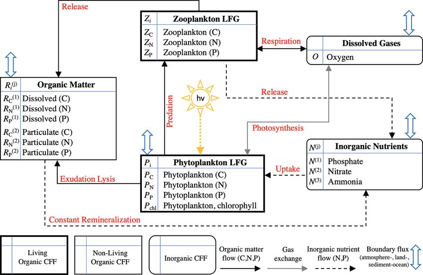
izations used in global and column models. This provides tracked in BFM17 is provided in Table 1, and a schematic of
motivation for the present study, since a primary goal in the the CFFs and LFGs used in BFM17, along with their inter-
development of BFM17 is to create a BGC model that can be actions, is shown in Fig. 1. The detailed equations compris-
used in combination with high-resolution, high-fidelity phys- ing BFM17, as well as all associated parameter values, are
ical models (e.g., those found in LES) to understand the ef- presented in Appendix A. Results from an initial 0-D test of
fects of these physical processes and how they can be more BFM17 are provided in Appendix B.
accurately represented in mixing parameterizations.
Dissolved and particulate organic matter, each with their
own partitions of carbon, nitrogen, and phosphate, are also 3 Coupled physical–biogeochemical flux model
included in BFM17 to account for nutrient recycling and car-
bon export due to particle sinking. Another primary goal of As a demonstration of BFM17 for predicting ocean biogeo-
developing BFM17 is to explore how spatially decoupled (or chemistry in oligotrophic pelagic zones, here we couple the
“patchy”) processes, such as the sinking of organic matter model to a 1-D physical mixing parameterization and make
and the subsequent upwelling of multiple recycled nutrients comparisons with available observational data in the Sar-
(not just nitrate) affect the fate and distribution of a phyto- gasso Sea. In order to focus on the upper-thermocline, open-
plankton bloom. ocean regime for which BFM17 was developed, the physical
Lastly, remineralization of nutrients is provided by param- model only extends 150 m in depth and diagnostically calcu-
eterized bacterial closure terms, thereby reducing complexity lates diffusivity terms based upon prescribed temperature and
while still maintaining critical nutrient recycling. The related salinity profiles from the observations. While a 1-D physical
parameter values (see Table A5 in Appendix A) were chosen model is unlikely to resolve all processes relevant for biogeo-
according to Mussap et al. (2016), who carried out sensitiv- chemistry in the upper thermocline, we have made additions,
ity tests to evaluate the many parameter values found in the such as large-scale general circulation and mesoscale eddy
literature. vertical velocities, as well as relaxation bottom boundary
Iron is omitted from BFM17, limiting the applicability of conditions for nutrient upwelling, to better represent missing
the model in regions where iron components are important, processes.
such as the Southern Ocean and the tropical Pacific. Thus, For all equations here and in Appendix A, we adopt the
if used in such regions, at least a fixed concentration of iron same notation style used for BFM56 in Vichi et al. (2007),
may be needed (although this method has not yet been val- Mussap et al. (2016), and the BFM user manual (Vichi et al.,
idated within BFM17). Top-down control of the ecosystem 2013) for consistency and clarity. The coupled physical and
in the form of explicit predation of zooplankton is also not BGC model is a time–depth model that integrates in time the
included. Instead, a simple constant zooplankton mortality generic equation for all biological state variables, denoted
is used, as this is a complicated process and understand- Aj , given by
ing where to add this closure and where to feed the partic-
∂Aj ∂Aj h i ∂A
j
ulate and dissolved nutrients from this process in a lower- = − W + WE + v (set)
complexity model is not well understood. However, the ad- ∂t ∂t bio ∂z
dition of a top-down closure term was tested, and no ma- ∂ ∂Aj
jor differences were observed in the model results. Conse- + KH , (1)
∂z ∂z
quently, it was assumed that the constant mortality term was
sufficient for this model, similar to other models of this com- where Aj are the 17 state variables of BFM17, the first term
plexity (Fasham et al., 1990; Lawson et al., 1996; Clainche on the right-hand side accounts for sources and sinks within
et al., 2004). Additionally, the benthic system within BFM56 each species due to biological and chemical reactions (as
(Mussap et al., 2016) has been removed. It is assumed that represented by the equations comprising BFM17 and out-
Geosci. Model Dev., 14, 2419–2442, 2021 https://doi.org/10.5194/gmd-14-2419-2021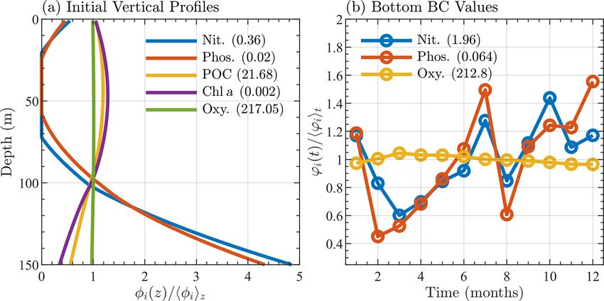
K. M. Smith et al.: A reduced biogeochemical flux model                                                                              2423

Table 1. Notation used for the 17 state variables in the BFM17 model, as well as the chemical functional family (CFF), units, description,
and rate equation reference for each state variable. CFFs are divided into living organic (LO), non-living organic (NO), and inorganic (IO)
families.

                             Symbol     CFF     Units             Description                       Equation
                             PC         LO      mg C m−3          Phytoplankton carbon                  (A5)
                             PN         LO      mmol N m−3        Phytoplankton nitrogen                (A6)
                             PP         LO      mmol P m−3        Phytoplankton phosphorus              (A7)
                             Pchl       LO      mg Chl a m−3      Phytoplankton chlorophyll             (A8)
                             ZC         LO      mg C m−3          Zooplankton carbon                   (A31)
                             ZN         LO      mmol N m−3        Zooplankton nitrogen                 (A32)
                             ZP         LO      mmol P m−3        Zooplankton phosphorus               (A33)
                               (1)
                             RC         NO      mg C m−3          Dissolved organic carbon             (A41)
                              (1)
                             RN         NO      mmol N m−3        Dissolved organic nitrogen           (A42)
                              (1)
                             RP         NO      mmol P m−3        Dissolved organic phosphorus         (A43)
                              (2)
                             RC         NO      mg C m−3          Particulate organic carbon           (A44)
                              (2)
                             RN         NO      mmol N m−3        Particulate organic nitrogen         (A45)
                              (2)
                             RP         NO      mmol P m−3        Particulate organic phosphorus       (A46)
                             O          IO      mmol O2 m−3       Dissolved oxygen                     (A47)
                             N (1)      IO      mmol P m−3        Phosphate                            (A48)
                             N (2)      IO      mmol N m−3        Nitrate                              (A49)
                             N (3)      IO      mmol N m−3        Ammonium                             (A50)

Figure 1. Schematic of the 17-state-equation BFM17 model. The dissolved organic matter, particulate organic matter, and living organic
matter CFFs are each comprised of three chemical constituents (i.e., carbon, nitrogen, and phosphorus). The living organic CFF is further
subdivided into phytoplankton and zooplankton living functional groups (LFGs).

https://doi.org/10.5194/gmd-14-2419-2021                                                   Geosci. Model Dev., 14, 2419–2442, 2021
2424                                                                  K. M. Smith et al.: A reduced biogeochemical flux model

lined in Appendix A), W and WE are the vertical veloci-               gradients and temperature are used in place of potential tem-
ties due to large-scale general circulation and mesoscale ed-         perature since we consider only the upper water column.
dies, respectively, v (set) is the settling velocity, and KH is          A detailed description of POM can be found in Blumberg
the vertical eddy diffusivity. Although the BFM17 formula-            and Mellor (1987), and in the following we simply provide
tion and model results are the primary focus of the present           a description of the physical model and equations solved in
study, we also perform coupled physical–BGC simulations               POM-1D. In diagnostic mode, as used in the present study,
using BFM56 for comparison. Equation (1) applies to all 17            POM-1D solves the momentum equations for U and V given
state variables in BFM17, as well as to all 56 state variables        by
in BFM56. Consequently, the only differences between the
biophysical models with BFM17 and BFM56 are the num-                  ∂U       ∂       ∂U
                                                                         −fV =      KM      ,                                     (2)
ber of state variables being tracked and the equations used           ∂t       ∂z      ∂z
to calculate the biological forcing terms. The specific forms         ∂V       ∂

                                                                                       ∂V

of Eq. (1) for each of the 17 species in BFM17 are dis-                  +fU =      KM      ,                                     (3)
                                                                      ∂t       ∂z      ∂z
cussed in Appendix A, and the specific forms of this equation
for each of the 56 species in BFM56 were previously dis-              where f = 2 sin φ is the Coriolis force,  is the angular ve-
cussed in Vichi et al. (2007). The parameters used in BFM56           locity of the Earth, and φ is the latitude. The vertical viscos-
correspond to the values provided in Tables A3–A5 of Ap-              ity KM and diffusivity KH are calculated using the closure
pendix A, with the remaining undefined parameters (since              hypothesis of Mellor and Yamada (1982) as
BFM56 includes many more model parameters than BFM17)
based on values from Mussap et al. (2016).                            KM = q l SM ,                                               (4)
   The range of values for W and WE in Eq. (1) is included in
Table 2 and the corresponding depth profiles are discussed in         KH = q l SH ,                                               (5)
Sect. 4.3. The settling velocity, v (set) , in Eq. (1) is only non-
zero for the three constituents of particulate organic matter,        where q is the turbulent velocity and SH and SM are stability
and its value is given in Table 2. We assume v (set) = 0 for          functions written as
zooplankton, since zooplankton actively swim and oppose                                          h                     i
their own sinking velocity. Finally, KH in Eq. (1) is calcu-          SM [1 − 9A1 A2 GH ] − SH (18A21 + 9A1 A2 )GH
lated by the model and is described in more detail later in
                                                                                            = A1 1 − 3C1 − 6A1 /B1 ,

                                                                                                                                (6)
this section.
   To obtain the complete 1-D biophysical model, BFM17                SH [1 − (3A2 B2 + 18A1 A2 )GH ] = A2 1 − 6A1 /B1 . (7)
has been coupled with a modification of the three-
dimensional (3-D) POM (Blumberg and Mellor, 1987) that                The coefficients in the above expressions are
considers only the vertical (specifically, the upper 150 m of         (A1 , B1 , A2 , B2 , C1 ) = (0.92, 16.6, 0.74, 10.1, 0.08), with
the water column) and time dimensions; that is, the evolution
of the system in the (z, t) space. It is well known that the                 l 2 g ∂ρ
                                                                      GH =             ,                                          (8)
primary calibration dimension in marine ocean biogeochem-                    q 2 ρ0 ∂z
istry is along the vertical direction, as shown in several pre-
vious calibration and validation exercises (Vichi et al., 2003;       where ρ0 = 1025 kg m−3 , g = 9.81 m s−2 . Following Mellor
Triantafyllou et al., 2003; Mussap et al., 2016).                     (2001), GH is limited to have a maximum value of 0.028.
   The 1-D POM solver (POM-1D) is used to calculate the               The equation of state relating ρ to T and S is non-linear
vertical structure of the two horizontal velocity components,         (Mellor, 1991) and given by
denoted U and V , the potential temperature, T , salinity,
S, density, ρ, turbulent kinetic energy, q 2 /2, and mixing           ρ = 999.8 + (6.8 × 10⁻² − 9.1 × 10⁻³ T
length scale, `. In this model adaptation, vertical tempera-            + 1.0 × 10⁻⁴ T 2 − 1.1 × 10⁻⁶ T 3 + 6.5 × 10⁻⁹ T 4 ) T
ture and salinity profiles are imposed from given climatolog-
ical monthly profiles obtained from observations, as previ-             + (0.8 − 4.1 × 10⁻³ T + 7.6 × 10⁻⁵ T 2
ously done in Mussap et al. (2016) and Bianchi et al. (2005).           − 8.3 × 10⁻⁷ T 3 + 5.4 × 10⁻⁹ T 4 )S
POM-1D directly computes the time evolution of the hori-
                                                                        + (−5.7 × 10⁻³ + 1.0 × 10⁻⁴ T
zontal velocity components, the turbulent kinetic energy and
the mixing length scale, all of which are used to compute               − 1.6 × 10⁻⁶ T 2 )S 1.5 + 4.8 × 10⁻⁴ S 2 ,                (9)
the turbulent diffusivity term, KH , required in Eq. (1). In this
configuration, POM-1D is called “diagnostic” since temper-            where the polynomial constants have been written only up
ature and salinity are prescribed. Furthermore, pressure ef-          to the first digit. For a more precise reproduction of these
fects are neglected in the density equation and the buoyancy          constants, the reader is referred to Mellor (1991). Finally, the
                                                                      governing equations solved to obtain the turbulence variables

Geosci. Model Dev., 14, 2419–2442, 2021                                                https://doi.org/10.5194/gmd-14-2419-2021
K. M. Smith et al.: A reduced biogeochemical flux model                                                                          2425

Table 2. Values, units, and descriptions for parameters used in the combined physical–BFM17 model.

                             Symbol       Value   Units     Description
                             v (set)    −1.00     m d−1     Settling velocity of particulate detritus
                             W         −0.02–0    m d−1     Imposed general circulation vertical velocity
                             WE          0–0.1    m d−1     Imposed mesoscale circulation vertical velocity
                             λO            0.06   m d−1     Relaxation constant for oxygen at bottom
                             λN (1)        0.06   m d−1     Relaxation constant for phosphate at bottom
                             λN (2)        0.06   m d−1     Relaxation constant for nitrate at bottom

q 2 /2 and ` are                                                        For all variables except oxygen, surface boundary condi-
                                                                     tions for the coupled model variable Aj are
 ∂ q2                 ∂ q2

               ∂
           =      Kq                                                         ∂Aj
∂t 2          ∂z     ∂z 2                                             KH                  = 0.                                    (16)
                 "               #                                          ∂z    z=0
                    ∂U 2      ∂V 2

           + KM           +                                          By contrast, the surface boundary condition for oxygen has
                     ∂z       ∂z
                                                                     the form
          g      ∂ρ     q3                                                   ∂O
            +KH      −     ,                                (10)      KH                  = 8O ,                                  (17)
          ρ0     ∂z B1 `                                                     ∂z
                                                                                  z=0
∂  2     ∂       ∂  2
   q ` =        Kq     q `                                           where 8O is the air–sea interface flux of oxygen computed
∂t        ∂z       ∂z
                   "                #                              according to Wanninkhof (1992, 2014). The bottom (i.e.,
                      ∂U 2       ∂V 2

                                                                     greatest depth) boundary conditions for phytoplankton, zoo-
        + E1 `KM             +
                      ∂z         ∂z                                  plankton, dissolved organic matter, and particulate organic
                                                                     matter are
                     g     ∂ρ q 3 e
            + E1 `      KH   −    W,                        (11)             ∂Aj
                     ρ0    ∂z B1                                      KH                     = 0.                                 (18)
                                                                              ∂z    z=zend
where Kq = κ KH is the vertical diffusivity for turbu-
lence variables, κ = 0.4 is the von Karman       constant, and      This boundary condition was chosen since it allows removal
We = 1 + E2 `2 /κ 2 (1/|z| + 1/|z − H |)2 with (E1 , E2 ) =
                                                                    of the scalar quantity Aj through the bottom boundary of
(1.8, 1.33). In Eqs. (10) and (11), the time rate of change          the domain. This can be seen by integrating Eq. (1) over the
of the turbulence quantities is equal to the diffusion of turbu-     boundary layer depth using the boundary condition above,
lence (the first term on the right-hand side of both equations),     giving
the shear and buoyancy turbulence production (second and                     Zz=0
third terms), and the dissipation (the fourth term). This is a        ∂                    h                i
                                                                                    Aj dz = W + WE + v (set) Aj    z=zend
                                                                                                                            ,     (19)
second-order turbulence closure model that was formulated             ∂t
                                                                           z=zend
by Mellor (2001) as a particular case of the Mellor and Ya-
mada (1982) model for upper-ocean mixing.                            where the biological part of Eq. (1) has been neglected and
   Boundary conditions for the horizontal velocities U =             the resulting temporal change in the integrated scalar Aj is
(U, V ) and the turbulence quantities are                            negative since |(W +WE )| < |v (set) |, as shown in Table 2. For
                                                                     oxygen, phosphate, and nitrate, the bottom boundary condi-
   ∂U
KM          = τw ,                                          (12)     tions are
    ∂z z=0
                                                                          ∂Aj
KM
   ∂U
              = 0,                                          (13)     KH               = λj Aj z=z − A∗j ,                        (20)
    ∂z z=zend                                                              ∂z z=zend               end


                   2/3 |τ w |                                        where λj and A∗j are the corresponding relaxation velocity

  2 2
 q ,q `       = B1            ,0 ,                          (14)
          z=0           Cd                                           and observed at-bottom boundary climatological field data
(q 2 , q 2 `)|z=zend = 0 ,                                  (15)     value, respectively, of that species. Base values for the relax-
                                                                     ation velocities are included in Table 2. Lastly, the bottom
where τ w = Cd |uw |uw is the surface wind stress, uw is the         boundary condition for ammonium is
surface wind vector, Cd is a constant drag coefficient chosen
to be 2.5 × 10⁻³ , and z = 0 and z = zend denote the locations               ∂N (3)
                                                                      KH                       = 0.                               (21)
of the surface and the greatest depth modeled, respectively.                  ∂z
                                                                                      z=zend

https://doi.org/10.5194/gmd-14-2419-2021                                                       Geosci. Model Dev., 14, 2419–2442, 2021
2426 K. M. Smith et al.: A reduced biogeochemical flux model
Since observations of ammonium concentration in the ob- for the BATS data and 23 years (not continuous) for the BTM
servational area are not available, this choice is based on data. Additionally, we interpolate the BATS data to a verti-
the assumption that the nitrogen diffusive flux from depth cal grid with 1 m resolution. We subsequently smooth the in-
to the surface (euphotic) layers occurs mostly in the form of terpolated data, using a robust locally estimated scatterplot
a nitrate flux, consistent with the concepts of “new” and “re- smoothing (LOESS) method, to maintain a positive buoy-
generated” production, as described by Dugdale and Goering ancy gradient, thereby eliminating any spurious buoyancy-
(1967) and Mulholland and Lomas (2008). driven mixing due to interpolation and averaging.
Figure 2 shows the monthly climatological profiles of tem-
perature and salinity from the BATS data (maximum mixed
4 Field validation and calibration data layer depth from the climatology is approximately 149 m,
which was calculated based upon a 0.2 kg m−3 increase in
4.1 Study site description
density from the surface value), as well as the PAR and
Field data for calibration and validation of BFM17 10 m wind speed from the BTM data. The same monthly
are taken from the Bermuda Atlantic Time-series Study averaging, vertical interpolations, and smoothing used for
(BATS) (Steinberg et al., 2001) and the Bermuda Testbed the physical variables are also performed for biological vari-
Mooring (BTM) (Dickey et al., 2001) sites, which are lo- ables, which largely serve as target fields for the validation
cated in the Sargasso Sea (31◦ 400 N, 64◦ 100 W) in the North of BFM17.
Atlantic subtropical gyre. Both sites are a part of the US Joint
4.3 Inputs to the physical model
Global Ocean Flux Study (JGOFS) program. Data have been
collected from the BATS site since 1988 and from the BTM The physical model computes density from the prescribed
site since 1994. temperature and salinity, and surface wind stress from the
Steinberg et al. (2001) provide an overview of the biogeo- 10 m wind speed; temperature, salinity, and wind speed are
chemistry in the general BATS and BTM area. Winter mixing all provided by the BATS/BTM data. The model also uses
allows nutrients to be brought up into the mixed layer, pro- these data in the turbulence closure to compute the turbulent
ducing a phytoplankton bloom between January and March viscosity and diffusivity. This diagnostic approach eliminates
(winter mixed layer depth is typically 150–300 m). As ther- any drifts in temperature and salinity that might occur due to
mal stratification intensifies over the summer months, this improper parameterizations of lateral mixing in a 1-D model,
nutrient supply is cut off (summer mixed layer depth is typi- therefore providing greater reliability. In addition to the 10 m
cally 20 m). At this point, a subsurface chlorophyll maximum wind speed, temperature, and salinity, BFM requires monthly
is observed near a depth of 100 m. Stoichiometric ratios of varying PAR at the surface. For all the monthly mean input
carbon, nitrate, and phosphate are often non-Redfield and, in datasets, a correction (Killworth, 1995) is applied. This cor-
contrast to many oligotrophic regimes, phosphate is the dom- rection is applied to the monthly averages to reduce the er-
inant limiting nutrient (Fanning, 1992; Michaels et al., 1993; rors incurred by linearly interpolating monthly averages to
Cavender-Bares et al., 2001; Steinberg et al., 2001; Ammer- the much shorter model time step.
man et al., 2003; Martiny et al., 2013; Singh et al., 2015). We imposed both general circulation, W , and mesoscale
eddy, WE , vertical velocities in the simulations. The imposed
4.2 Data processing
vertical profiles of these velocities have been adapted from
The region encompassing the BATS and BTM sites is char- Bianchi et al. (2005), where the velocities are assumed to
acterized as an open-ocean oligotrophic region that is phos- be zero at the surface and reach their maxima near the base
phate limited. This region has thus been chosen for ini- of the Ekman layer, which is assumed to be at or below the
tial testing of BFM17 due to the prevalence of oligotrophic bottom boundary of the simulations. The general large-scale
regimes in the open ocean and to demonstrate the ability upwelling or downwelling circulation, W , is due to Ekman
of BFM17 to capture difficult non-Redfield ratio regimes pumping and is correspondingly given as
(which occur in phosphate-limited regions). The BATS/BTM
τw
data have also been collected over many years, providing W = k̂ · ∇ × , (22)
ρf
long time series for model calibration and validation.
Data from the BATS/BTM area are used in the present where k̂ denotes the unit vector in the vertical direction.
study for two purposes: (i) as initial, boundary, and forc- The monthly average value and sign of the wind stress curl,
ing conditions for the POM-1D biophysical simulations with ∇ × τ w , for the general BATS/BTM region is taken from the
BFM17 and BFM56, and (ii) as target fields for validation of Scatterometer Climatology of Ocean Winds database (Risien
the simulations. In addition to the subsurface BATS data, we and Chelton, 2008, 2011). The monthly value of W from
also use BTM surface data, such as the 10 m wind speed and Eq. (22) is then assumed to be the maximum, occurring at
photosynthetically active radiation (PAR). For each observa- the base of the Ekman layer, for that particular month. Given
tional quantity, we compute monthly averages over 27 years the sign of the wind stress curl for the BATS/BTM region, a
Geosci. Model Dev., 14, 2419–2442, 2021 https://doi.org/10.5194/gmd-14-2419-2021K. M. Smith et al.: A reduced biogeochemical flux model 2427
Figure 2. Sargasso Sea physical variables, showing climatological monthly averaged (a) temperature, (b) 10 m surface wind speed, (c) surface
PAR, and (d) salinity. Panel (e) shows the mean seasonal general circulation velocity, W , and panel (f) shows the bimonthly maximum value
of the mesoscale eddy velocity WE . Monthly averaged mixed layer depths (defined as the depth at which the density is 0.2 kg m−3 greater
than the surface density) are shown as black lines in panel (a).
negative W was calculated, indicating general downwelling termined either through the adoption of the Redfield ratio
processes in this region. Seasonal profiles of W are shown in C : N : P ≡ 106 : 16 : 1 (Redfield et al., 1963) or assuming a
Fig. 2e. reasonably low initial value. Since the 1-D simulations were
Due to the prevalence of mesoscale eddies within the run to steady state over 10 years, memory of these initial
BATS/BTM region (Hua et al., 1985), which can provide states was assumed to be lost, with little effect on the results.
episodic upwelling of nutrients to the upper water column, For the comparison of BFM17 to BFM56, the initial con-
we also include an additional positive upwelling vertical ve- ditions for the additional state variables were calculated by
locity, WE , which has a timescale of 15 d. The general profile splitting the total initial phytoplankton and zooplankton car-
of WE is assumed to be the same as for W , with a value of bon values into equal amounts for all phytoplankton and zoo-
zero at the surface and a maximum value at depth. However, plankton groups. The other state variables for each group
there is no linear interpolation between each 15 d period, and were again calculated using the Redfield ratio. The initial
the maximum magnitude of WE is randomized between 0 and bacteria distribution was defined by setting the column equal
0.1 m d−1 , as shown in Fig. 2f for each 15 d period. to a constant value.
In both simulations, the bottom boundary conditions for
4.4 Initial and boundary conditions oxygen, nitrate, and phosphate species are based on observed
BATS data. Values are taken at the next closest data point
Although the BATS/BTM data include information on many below the bottom boundary (at 150 m) and then averaged
biological variables, initial conditions for only 5 of the 17 over the month. Figure 3b shows the monthly average bot-
species within BFM17 could be extracted from the data. Sim- tom boundary conditions for each of the three species.
ilarly to the temperature and salinity, the initial chlorophyll,
particulate organic nitrogen, oxygen, nitrate, and phosphate
were interpolated to a mesh with 1 m vertical grid spacing, 5 Model assessment results
averaged over the initial month of January, and smoothed
vertically in space to give the initial profiles seen in Fig. 3a. The coupled BFM17-POM-1D model was run using the pa-
The remaining 12-state-variable initial conditions were de- rameter values from Tables 2, A1, and A3–A5, which were
https://doi.org/10.5194/gmd-14-2419-2021 Geosci. Model Dev., 14, 2419–2442, 20212428 K. M. Smith et al.: A reduced biogeochemical flux model
Figure 3. Sargasso Sea initial and boundary conditions showing (a) initial profiles of nitrate, phosphate, particulate organic carbon, chloro-
phyll, and oxygen, where each profile, denoted φi (z), is normalized by its depth averaged value, hφi iz , and (b) monthly bottom boundary
conditions for nitrate, phosphate, and oxygen, where each quantity, ϕi (t), is normalized by its annual average value hϕi it . The depth and
annual averaged values are shown in parentheses in the legends of each panel. Units are mmol N m−3 for nitrate, mmol P m−3 for phosphate,
mg C m−3 for particulate organic carbon, mg Chl m−3 for chlorophyll, and mmol O m−3 for oxygen.
decided on the basis of standard literature values (Vichi et al., brated to give reasonable agreement with the observational
2007, 2003, 2013; Fiori et al., 2012). The simulations were data.
allowed to run out to steady state, and multi-year monthly As mentioned previously, oxygen is historically difficult
means were calculated as functions of depth for chloro- to predict using BGC models of any complexity. It is likely
phyll, oxygen, nitrate, phosphate, particulate organic nitro- that this is due, in part, to inaccuracies in the mixing pa-
gen (PON), and net primary production (NPP), each of which rameterizations used in POM-1D and other physical models.
was measured at the BATS/BTM site. The model PON is For example, BFM17 struggles to accurately predict oxygen,
defined as the sum of nitrogen contained within the phyto- in part, because the second-order mixing scheme of Mellor
plankton, zooplankton, and particulate detritus, and NPP is and Yamada (1982) lacks sufficient resolution of the winter
defined as the net phytoplankton carbon uptake (or gross pri- mixing using just the monthly mean temperature and salin-
mary production) minus phytoplankton respiration. ity. However, since it is often not included or presented at
Figure 4 qualitatively compares the BATS data (top row) all in models of similar complexity to BFM17 (i.e., models
with the results from BFM17 (middle row). The model is reduced enough to reasonably couple to a high-fidelity, high-
able to capture the initial spring bloom between January resolution physical model), studies that explore this hypothe-
and March brought on by physical entrainment of nutrients, sis have been difficult to undertake. Thus, we include oxygen
the corresponding peak in net primary production and PON in BFM17 and present our results here to illustrate this ex-
around the same time, and the subsequent subsurface chloro- act point and to lend motivation to developing and using a
phyll maxima during the summer (evident in Fig. 4 as a larger model such as BFM17 to study the effects of physical pro-
chlorophyll concentration at depths close to 100 m during the cesses missing from mixing parameterizations and how they
summer months). The predicted oxygen levels are lower than can be better represented.
observed values; however, the overall structure predicted by To obtain a first indication of the performance of BFM17,
BFM17 is not completely dissimilar to that of the BATS a model assessment was performed for each target field. The
oxygen field. These results are consistent with those from same assessment was performed for BFM56 to compare the
BFM56 (bottom row of Fig. 4), suggesting that the two mod- two models. The results are summarized by the Taylor dia-
els are in generally close agreement. Correlation coefficients gram in Fig. 5. This diagram can be used to assess the extent
between the two models are 0.85 for chlorophyll, 0.56 for of misfit between the models and observations by showing
oxygen, 0.99 for nitrate, 0.99 for phosphate, 0.95 for PON, the normalized root mean square errors (RMSEs), normal-
and 0.97 for NPP. Differences in chlorophyll and oxygen are ized standard deviation, and the correlation coefficient be-
likely due to the removal in BFM17 of specific phytoplank- tween each of the model outputs and the BATS target fields.
ton and zooplankton species in favor of general LFGs, to The normalized RMSEs were calculated as εrms /σobs ,
the removal of denitrification, and to the parameterization where εrms is the RMSE between the model and the obser-
of remineralization using new closure terms that were cali- vation fields and σobs is the standard deviation of the obser-
vation field. The normalized standard deviation was calcu-
Geosci. Model Dev., 14, 2419–2442, 2021 https://doi.org/10.5194/gmd-14-2419-2021K. M. Smith et al.: A reduced biogeochemical flux model 2429
Figure 4. Comparison of target BATS fields (a–f) to BFM17 simulation results (g–l) and BFM56 simulation results (m–r) for (a ,g, m) chloro-
phyll (mg Chl a m−3 ), (b, h, n) oxygen (mmol O m−3 ), (c, i, o) nitrate (mmol N m−3 ), (d, j, p) phosphate (mmol P m−3 ), (e, k, q) particulate
organic nitrogen (PON; mg N m−3 ), (f, l, r) and net primary production (NPP; mg C m−3 d−1 ). Simulation plots are multi-year monthly
averages of the last 3 years of a 10-year integration.
lated as σmod /σobs , where σmod is the standard deviation of while NPP and PON have too little and too much variability,
the model fields. The normalized RMSEs, normalized stan- respectively.
dard deviation, and the correlation coefficients each give an Table 3 provides a comparison of correlation coefficients
indication of the relative similarities in amplitude, variations and un-normalized RMSEs, calculated with respect to the
in amplitude, and structure of each modeled field compared observational fields, from BFM17 and BFM56, as well as
to the BATS target fields, respectively. For each variable, from other models. Comparisons were only made to models
these statistics were calculated over all months and all depths that were calibrated using the same BATS/BTM data, em-
shown in Fig. 4. ployed some kind of parameter estimation technique, and re-
The Taylor diagram in Fig. 5 shows that BFM17 and ported correlation and RMSEs. Ayata et al. (2013) included
BFM56 produce similar results. For most variables, errors six biological tracers, while both Fasham et al. (1990) and
in the amplitudes are within roughly one standard devia- Spitz et al. (2001) included seven. The Spitz et al. (2001)
tion of the observations. Additionally, the structures of the study used data assimilation, while the Ayata et al. (2013)
model fields for chlorophyll, nitrate, phosphate, PON, and and Fasham et al. (1990) studies used only optimization to
NPP have high correlations with that of the BATS target determine a select set of parameters. All models used clima-
fields. The correlation values range from 0.63 for chlorophyll tological monthly mean forcing from the BATS region and
to 0.94 for nitrate in BFM17 and from 0.60 for chlorophyll reported climatological monthly means for their results. Care
to 0.93 for phosphate and nitrate in BFM56. For BFM17, was taken to ensure that the same variable definition was
variabilities in amplitude for nitrate, phosphate, oxygen, and compared between all models. Ayata et al. (2013) used a sim-
NPP are closest to those of the corresponding BATS target ilar 1-D physical model to the one that was used here, while
fields, while the chlorophyll and PON have too much vari- Spitz et al. (2001) and Fasham et al. (1990) used a time-
ability. For BFM56, nitrate, phosphate, oxygen, and chloro- dependent box model of the upper-ocean mixed layer. As
phyll have similar variability in amplitude to the BATS data, such, correlations and RMSE values for comparison to Ay-
ata et al. (2013) were computed over the entire domain (Ay-
https://doi.org/10.5194/gmd-14-2419-2021 Geosci. Model Dev., 14, 2419–2442, 20212430 K. M. Smith et al.: A reduced biogeochemical flux model
as the Spitz et al. (2001) model. The extra biological trac-
ers in BFM17, as compared to the Ayata et al. (2013) and
Fasham et al. (1990) models, account for variable intra- and
extracellular nutrient ratios with the addition of phosphorus.
Finally, a key benefit of the chemical functional family ap-
proach used by BFM17 is the ability of the model to predict
non-Redfield nutrient ratios. Figure 6 shows the constituent
component ratios normalized by the respective Redfield ra-
tios for BFM17. The figure includes the component ratios
of carbon to nitrogen, carbon to phosphorous, and nitrogen
to phosphorous for phytoplankton, dissolved organic matter
(DOM), and POM. Zooplankton nutrient ratios were not in-
cluded because the parameterization of the zooplankton re-
Figure 5. Taylor diagram showing the normalized standard devia- laxes the nutrient ratio back to a constant value. The normal-
tion, correlation coefficient, and normalized root mean squared dif- ized ratio values are uniform non-unity-valued fields.
ferences between the BFM17 output and the BATS target fields. Ultimately, Fig. 6 shows that BFM17 is able to cap-
Observations lie at (1,0). Radial deviations from observations cor- ture the phosphate-limited dynamics that characterize the
respond to the normalized root mean square error (RMSE), radial
BATS/BTM region (Fanning, 1992; Michaels et al., 1993;
deviations from the origin correspond to the normalized standard
deviation, and angular deviations from the vertical axis correspond
Cavender-Bares et al., 2001; Steinberg et al., 2001; Ammer-
to the correlation coefficient. BFM17 and BFM56 results are shown man et al., 2003; Martiny et al., 2013; Singh et al., 2015).
as colored circles and triangles, respectively (chlorophyll is indi- In particular, Fig. 6 shows that all results comparing carbon
cated in blue, oxygen is indicated in orange, nitrate is indicated in or nitrogen to phosphorous for BFM17 produce normalized
yellow, phosphate is indicated in purple, PON is indicated in green, values greater than 1, where the normalization is carried out
and NPP is indicated in cyan). Note that BFM56 nitrate and phos- using the Redfield ratio (i.e., a normalized value greater than
phate data points fall on top of one another (yellow and purple tri- 1 indicates that the field is denominator limited). Figure 6
angles). also shows that the ratios are not uniform for phytoplankton,
DOM, and POM, with the ratios decreasing with depth as a
result of the increased availability of nitrogen and phosphate.
ata et al., 2013, calculated their metrics over the top 168 m
of their domain). For comparison to Spitz et al. (2001) and
Fasham et al. (1990), correlations and RMSEs were calcu- 6 Conclusions
lated only within the mixed layer (defined as the depth at
which the density is 0.2 kg m−3 greater than the surface den- In this study, we have presented a new upper-thermocline,
sity) and are shown as separate columns in Table 3. open-ocean BGC model that is complex enough to capture
The correlation coefficients and RMSEs for both BFM17 open-ocean ecosystem dynamics within the Sargasso Sea re-
and BFM56 are comparable to the Ayata et al. (2013) study gion, yet reduced enough to integrate with a physical model
for chlorophyll, while they outperform this study for nitrate, with limited additional computational cost. The new model,
PON, and NPP. The Spitz et al. (2001) study, which used data named the Biogeochemical Flux Model 17 (BFM17), in-
assimilation and is therefore naturally more likely to perform cludes 17 state variables and expands upon more reduced
better, does in fact do so for predictions of chlorophyll and BGC models by incorporating a phosphate equation and
nitrate. However, the nitrate correlation values for BFM17 tracking dissolved oxygen, as well as variable intra- and
and the Spitz et al. (2001) model are both high, although extracellular nutrient ratios. BFM17 was developed primar-
the latter model does have a lower RMSE value. As com- ily for use within high-resolution, high-fidelity 3-D physical
pared to the Spitz et al. (2001) model, BFM17 has higher models, such as LES, for process, parameterization, and pa-
correlation values for both PON and NPP but a larger RMSE rameter optimization studies, applications for which its more
for NPP. Lastly, both BFM17 and BFM56 outperform the complex counterpart (BFM56) would be much too costly.
Fasham et al. (1990) study for all fields for both correlation To calibrate and test the model, it was coupled to the
coefficient and RMSE values. 1-D Princeton Ocean Model (POM-1D) and forced using
These results show that, with a relatively small increase field data from the Bermuda Atlantic test site area. The full
in the number of biological tracers as compared to simi- 56-state-variable Biogeochemical Flux Model (BFM56) was
lar models, BFM17 is generally able to increase correlation also run using the same forcing. Results were compared be-
coefficient values and decrease RMSE values for many of tween the two models and all six of the BATS target fields
the target fields in comparison to similar models. Moreover, – chlorophyll, oxygen, nitrate, phosphate, PON, and NPP –
BFM17 approaches the accuracy of models that use data as- and a model skill assessment was performed, concluding that
similation to improve agreement with the observations, such the BFM17 captures the subsurface chlorophyll maximum
Geosci. Model Dev., 14, 2419–2442, 2021 https://doi.org/10.5194/gmd-14-2419-2021K. M. Smith et al.: A reduced biogeochemical flux model 2431
Table 3. Correlation coefficients (and RMSE in parenthesis) between BATS target fields and model data for BFM17, BFM56, and several
example models of similar complexity. The first set of BFM columns is calculated over the entire water column, while the second set (denoted
with “ML only”) is calculated over the monthly mixed layer depth only (defined as the depth at which the density is 0.2 kg m−3 greater than
the surface density).
Variable BFM17 BFM56 Ayata et al. (2013) BFM17 BFM56 Fasham et al. Spitz et al.
(ML only) (ML only) (1990) (2001)
Chlorophyll 0.63 (0.08) 0.60 (0.10) 0.60 (0.06) 0.63 (0.07) 0.60 (0.09) −0.33 (0.34) 0.86 (0.04)
Oxygen 0.37 (31.18) 0.18 (21.84) – 0.29 (29.53) −0.09 (20.22) – –
Nitrate 0.94 (0.22) 0.93 (0.16) 0.80 (0.33) 0.94 (0.22) 0.93 (0.15) 0.87 (0.28) 0.98 (0.05)
Phosphate 0.91 (0.01) 0.93 (0.005) – 0.91 (0.01) 0.93 (0.005) – –
PON 0.85 (0.15) 0.85 (0.11) 0.45 (0.08) 0.86 (0.14) 0.86 (0.10) 0.48 (0.6) 0.76 (0.12)
NPP 0.93 (0.26) 0.87 (0.63) 0.50 (0.14) 0.94 (0.21) 0.89 (0.5) −0.47 (0.021) 0.69 (0.016)
Figure 6. Fields of BFM17 constituent component ratios of carbon to nitrogen (a–c), carbon to phosphorous (d–f), and nitrogen to phospho-
rous (g–i) for phytoplankton (a, d, g), dissolved organic detritus (b, e, h), and particulate organic detritus (c, f, i). Each field is normalized by
the respective Redfield ratio.
and bloom intensity observed in the BATS data and produces fields. Additionally, it would be useful to study the efficacy
comparable results to BFM56. In comparison with similar of using BFM17 in a global context, to reproduce the ecology
studies using slightly less complex models, BFM17-POM- in other regions of the ocean, and its sensitivity under various
1D performs on par with, or better than, those studies. physical forcing scenarios. Finally, BFM17 is now of a size
In the future, a sensitivity study is necessary to assess the that it can be efficiently integrated in high-resolution, high-
most sensitive model parameters, both in BFM17 as well fidelity 3-D simulations of the upper ocean, and future work
as in the 1-D physical model. After identification of these will examine model results in this context.
most sensitive model parameters, an optimization can be per-
formed to reduce discrepancies between the BATS obser-
vational biology fields and the corresponding model output
https://doi.org/10.5194/gmd-14-2419-2021 Geosci. Model Dev., 14, 2419–2442, 2021You can also read