MEANINGFULLY DEBUGGING MODEL MISTAKES US- ING CONCEPTUAL COUNTERFACTUAL EXPLANATIONS - ing conceptual ...
←
→
Page content transcription
If your browser does not render page correctly, please read the page content below
Under review as a conference paper at ICLR 2022
M EANINGFULLY DEBUGGING MODEL MISTAKES US -
ING CONCEPTUAL COUNTERFACTUAL EXPLANATIONS
Anonymous authors
Paper under double-blind review
A BSTRACT
Understanding and explaining the mistakes made by trained models is critical
to many machine learning objectives, such as improving robustness, addressing
concept drift, and mitigating biases. However, this is often an ad hoc process
that involves manually looking at the model’s mistakes on many test samples and
guessing at the underlying reasons for those incorrect predictions. In this paper, we
propose a systematic approach, conceptual counterfactual explanations (CCE), that
explains why a classifier makes a mistake on a particular test sample(s) in terms of
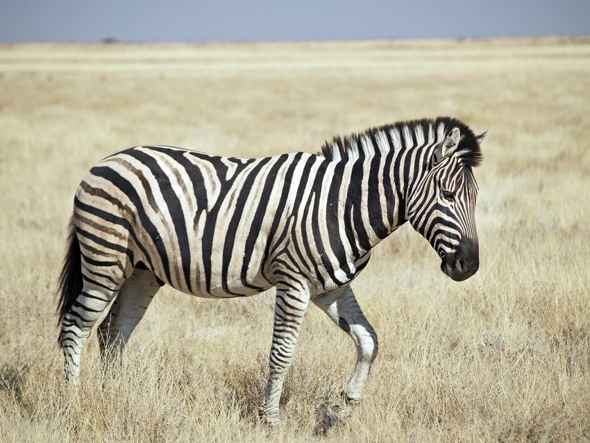
human-understandable concepts (e.g. this zebra is misclassified as a dog because
of faint stripes). We base CCE on two prior ideas: counterfactual explanations and
concept activation vectors, and validate our approach on well-known pretrained
models, showing that it explains the models’ mistakes meaningfully. In addition, for
new models trained on data with spurious correlations, CCE accurately identifies
the spurious correlation as the cause of model mistakes from a single misclassified
test sample. On two challenging medical applications, CCE generated useful
insights, confirmed by clinicians, into biases and mistakes the model makes in
real-world settings. The code for CCE is publicly available and can easily be
applied to explain mistakes in new models.
1 I NTRODUCTION
People who use machine learning (ML) models often need to understand why a trained model
is making a particular mistake. For example, upon seeing a model misclassify an image, an ML
practitioner may ask questions such as: Was this kind of image underrepresented in my training
distribution? Am I preprocessing the image correctly? Has my model learned a spurious correlation
or bias that is hindering generalization? Answering this question correctly affects the usability of a
model and can help make the model more robust. Consider a motivating example:
Example 1: Usability of a Pretrained Model. A pathologist downloads a pretrained model to
classify histopathology images. Despite a high reported accuracy, he finds the model performing
poorly on his images. He investigates why that is the case, finding that the hues in his images are
different than in the original training data. Realizing the issue, he is able to transform his own images
with some preprocessing, matching the training distribution and improving the model’s performance.
In the above example, we have a domain shift occurring between training and test time, which
degrades the model’s performance (Subbaswamy et al., 2019; Koh et al., 2020). By explaining the
cause of the domain shift, we are able to easily fix the model’s predictions. On the other hand, if the
domain shift is due to more complex spurious correlations the model has learned, it might need to
be completely retrained before it can be used. During development, identifying and explaining a
model’s failure points can also make it more robust (Abid et al., 2019; Kiela et al., 2021), as in the
following example:
Example 2: Discovering Biases During Development. A dermatologist trains a machine learning
classifier to classify skin diseases from skin images collected from patients at her hospital. She shares
her trained model with a colleague at a different hospital, who reports that the model makes many
mistakes with his own patients. She investigates why the model is making mistakes, realizing that
patients at her colleague’s hospital have different skin colors and ages. Answering this question
allows her to not only know her own model’s biases but also guides her to expand her training set
with the right kind of data to build a more robust model.
1
Under review as a conference paper at ICLR 2022

Explaining a model’s mistakes is also useful in other settings where data distributions may change,
such as concept drift for deployed machine learning models (Lu et al., 2018). Despite its usefulness,
explaining a model’s performance drop is often an ad hoc process that involves manually looking at
the model’s mistakes on many test samples and guessing at the underlying reasons for those incorrect
predictions. We present counterfactual conceptual explanations (CCE), a systematic method for
explaining model mistakes in terms of meaningful human-understandable concepts, such as those in
the examples above (e.g. hues). In addition, CCE was developed with the following criteria:

       • No training data or retraining: CCE does not require access to the training data or model
         retraining.
       • Only needs the model: CCE only needs white-box access to the model. The user can use
         any dataset to learn desired concepts.
       • High-level explanations: CCE provides high-level explanations of model mistakes using
         concepts that are easy for users to understand.

                                             Generating Conceptual
      a)   Learning a Concept Bank   b)                                    c) Explaining Model Mistake
                                                Counterfactuals
                                          Zebra

                                                                                African hunting dog (66%)

                                                                               Correct label → Zebra

                                                                             Stripes                         1.00

                                                  African                    Cow                             0.52
                                                  Hunting Dog                Polka Dots                      -0.2

                   ...                                                       Dog                            –0.35
                                                   → Concept explanation

Figure 1: Explaining with Conceptual Counterfactuals: (a) In generating conceptual explanations,
the first step is to define a concept library. After defining a concept library, we then learn a concept
activation vector (CAV) (Kim et al., 2018) for each concept. (b) Given a misclassified sample, such
as the Zebra image shown here as an African hunting dog, we would like to generate a conceptual
counterfactual. Meaning that we would like to generate a perturbation in the embedding space that
would correct the model prediction, using a weighted sum of our concept bank. (c) Our method
assigns a score to the set of concepts. A large positive score means that adding that concept to the
image (e.g. stripes) will increase the probability of correctly classifying the image, as will removing
or reducing a concept with a large negative score (e.g. polka dots or dogness).

Fig. 1 provides an overview of our CCE method. To summarize our contributions, we develop a
novel method, CCE, that can systematically explain model mistakes in terms of high-level concepts
that are easy for users to understand. We show that CCE correctly identifies spurious correlations
in model training, and we quantitatively validate CCE across different experiments over natural
and clinical images. We have released all of the code and data needed for our method in a public
repository: https://github.com/conceptualcounterfactuals/iclr2022.

2    R ELATED W ORKS
CCE is inspired by prior efforts to explain machine learning models’ predictions. Two ideas are
particularly relevant: counterfactual explanations and concept activation vectors. Here, we provide
an overview of these methods and discuss the differences between them and our proposed approach.

Counterfactual Explanations Counterfactual explanations (Verma et al. (2020) provides a com-
prehensive review) are a class of model interpretation methods that seek to answer: what perturbations
to the input are needed for a model’s prediction to change in a particular way? A large number
of counterfactual explanation methods have been proposed with various desiderata such as sparse
perturbations (Wachter et al., 2017), perturbations that remain close to the data manifold (Dhurandhar

                                                       2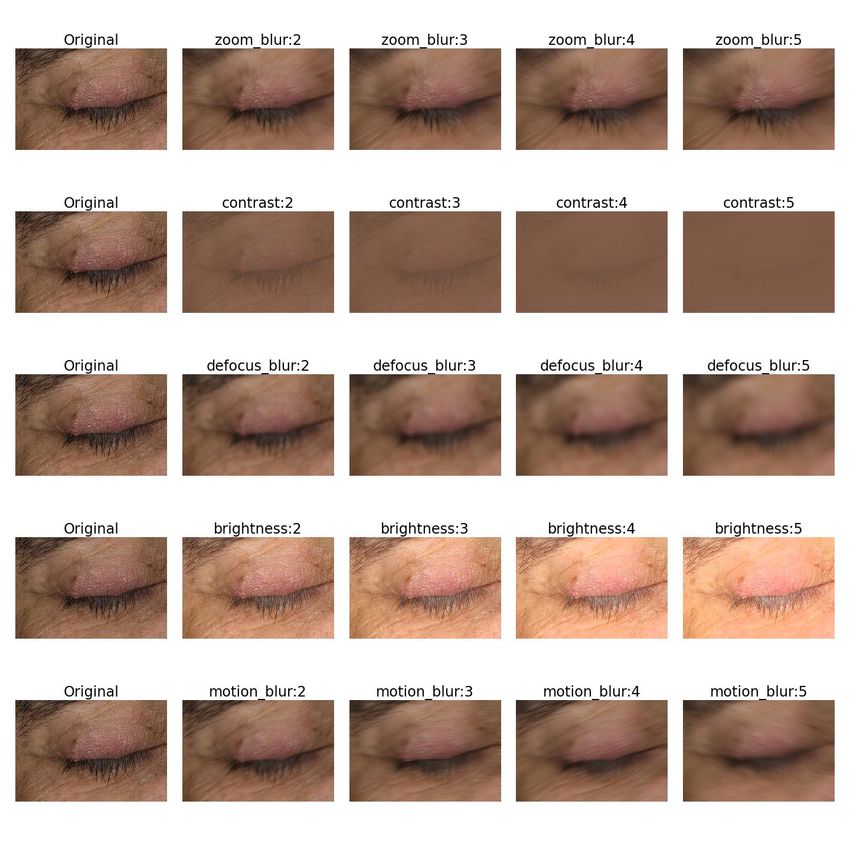
Under review as a conference paper at ICLR 2022

et al., 2018), and causality (Mahajan et al., 2019). What these methods share in common is that they
provide an interpretable link between model predictions and perturbations to input features. There
are several works focusing on counterfactual explanations for image data(Goyal et al., 2019; Singla
et al., 2020) and many of these methods use distractor images or modify input images to explain the
model behavior. However, perturbations or saliency maps in the input space are shown to be tricky to
interpret and be adopted by users(Alqaraawi et al., 2020; Adebayo et al., 2018).
To compute CCE, we use a similar approach, perturbing input data to change its predictions, but for
a complementary goal: to understand the limitations and biases of our model and its training data,
rather than to change a specific prediction. Further improving upon existing work, we do this by
directly using human-interpretable concepts, without having access to training data.

Concept Activation Vectors To explain an image classification model’s mistakes in a useful way,
we need to operate not with low-level features, but with more meaningful concepts. Concept activation
vectors (CAVs) (Kim et al., 2018) are a powerful method to understand the internals of a network
in human-interpretable concepts. CAVs are linear classifiers trained in the bottleneck layers of a
network and correspond to concepts that are usually user-defined or automatically discovered from
data (Ghorbani et al., 2019). Unlike many prior interpretation methods, explanations produced
by CAVs are in terms of high-level, human-understandable concepts rather than individual pixels
(Simonyan et al., 2013; Zhou et al., 2016) or training samples (Koh & Liang, 2017).
In previous literature, CAVs have been used to test the association between a concept and the model’s
prediction on a class of training data (Kim et al., 2018) as well as provide visual explanations for
predictions (Zhou et al., 2018). Our approach extends CAVs by showing that perturbations along
the CAV can be used to change a model’s prediction on a specific test sample, e.g. to correct a
mistaken prediction, and thereby be used in a similar manner to counterfactuals. Since samples (even
of the same class) can be misclassified for different reasons (see Fig. 6), our approach allows a more
contextual understanding of a model’s behavior and mistakes.

Bias/Error Detection and Robustness Understanding a model’s behavior and explaining its mis-
takes is critical for building more robust and less biased models, as we have discussed in Section 1.
While some other methods, such as FairML (Adebayo & Kagal, 2016) and the What-If Tool (Wexler
et al., 2020), can also be used to discover biases and failure points in models, they are typically limited
to tabular datasets where sensitive features are explicitly designated, unlike our approach which is
designed for unstructured data and works with a more flexible and diverse set of concepts. In a similar
spirit to our work, Singh et al. (2020) aim to identify and mitigate contextual bias, however, they
assume access to the whole training setup and data; which is a limiting factor in practical scenarios.
Our approach can also be used to explain a model’s performance degradation with data drift. It is
complementary to methods for out-of-distribution sample detection (Hendrycks & Gimpel, 2016)
and black-box shift detection (Lipton et al., 2018), which can detect data drift, but cannot explain
the underlying reasons. There are also algorithmic approaches to improve model robustness with
data drift (Raghunathan et al., 2018; Nestor et al., 2019). Although these methods can provide some
guarantees around robustness for unstructured data, they are in terms of low-level perturbations and
do not hold with more conceptual and natural changes in data distributions. There are several recent
methods for detecting clusters of mistakes made by a model (Kim et al., 2019; d’Eon et al., 2021),
which is useful for detecting disparity in the model, for example. CCE differs in that instead of
finding mistake clusters, CCE explains errors from just one (or a few) image.

3    M ETHODS

In this section, we detail the key steps of our method. Let us define basic notations: let f : Rd → Rk
be a deep neural network, let x ∈ Rd be a test sample belonging to class y ∈ {1, . . . k}. We assume
that that the model misclassifies x, meaning that arg maxi f (x)i 6= y or simply that the model’s
confidence in class y, f (x)y , is lower than desired. Let m be the dimensionality of the bottleneck
layer L, and bL : Rd → Rm be the “bottom” of the network, which maps samples from the input
space to the bottleneck layer, and tL : Rm → Rk be the “top” of the network, defined analogously.
For readability, we will usually underline class names and italicize concepts throughout this paper.

                                                    3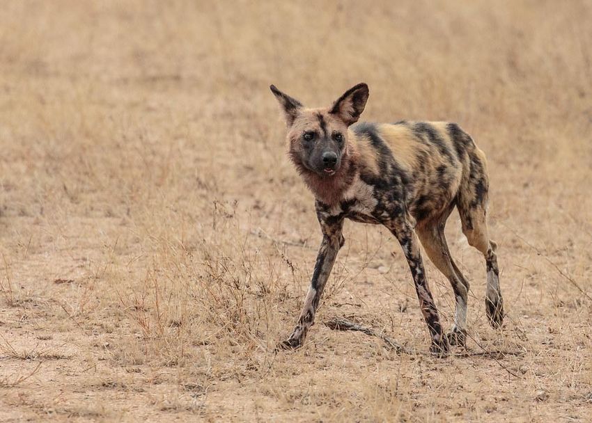
Under review as a conference paper at ICLR 2022

3.1   L EARNING C ONCEPTS

In generating conceptual explanations, the first step is to define a concept library: a set of human-
interpretable concepts C = {c1 , c2 , ...} that occur in the dataset. For each concept, we collect positive
examples, Pci , that exhibit the concept, as well as negative examples, Nci , in which the concept is
absent. Unless otherwise stated, we use Pci = Nci = 100. These concepts can be defined by the
researcher, by non-ML domain experts, or even learned automatically from the data (Ghorbani et al.,
2019). Since concepts are broadly reusable within a data domain, they can also be shared among
researchers. For our experiments with natural images, we defined 170 general concepts that include
(a) the presence of specific objects (e.g. mirror, person), (b) settings (e.g. street, snow) (c) textures
(e.g. stripes, metal), and (d) image qualities (e.g. blurriness, greenness). Many of our concepts were
adapted from the BRODEN dataset of visual concepts (Fong & Vedaldi, 2018). Note that the data
used to learn concepts can differ from the data used to train the ML model that we evaluate.
After defining a concept library, we then learn an SVM and the corresponding CAV for each concept.
We follow the same procedure as in (Kim et al., 2018), for the penultimate layer of a ResNet18
pretrained in ImageNet. This step only needs to be done once for each model that we want to evaluate,
and the CAVs can then be used to explain any number of misclassified samples. We refer the reader
to Appendix A.1 for implementational details and Appendix B for a full list of concepts. We denote
the vector normal to the classification hyperplane boundary as ci (normalized, i.e. |ci | = 1) and
the intercept of the SVM as φi . To measure whether concepts are successfully learned, we keep a
hold-out validation set and measure the validation accuracy, disregarding concepts with accuracies
below a threshold (0.7 in our experiments, which left us with 168 of the 170 concepts). We provide
more details about the threshold in Appendix B.

3.2   C ONCEPTUAL C OUNTERFACTUAL E XPLANATIONS

Drawing inspiration from the counterfactual explanations literature (Verma et al., 2020), we generate
a perturbation for a given misclassified test sample by varying the amount of different concepts in a
way such that the perturbation satisfies the following principles:
      1. Correctness: A counterfactual is considered correct if it achieves a desired outcome. In our
         case, this would mean that the perturbed test point should be classified as the correct label.
      2. Validity: We would like our counterfactuals to be valid, such that they would not violate
         real-world conditions. In our case, this means ensuring that the perturbed points contain
         realistic levels of each concept, as discussed below.
      3. Sparsity: The ultimate goal of generating explanations is communicating them to users. An-
         alyzing a large number of modifications and interactions may not be trivial, so perturbations
         should change a small number of concepts.
Let LCE denote the cross entropy loss. Using the concept vectors and intercepts (ci , φi )(see 3.1),
we build our concept bank C ∈ RNc ×m , φ ∈ RNc where Nc is the number of concepts and
m is the output dimension of the bottleneck layer. As our goal is to come up with a scoring
scheme for concepts, we need to define what it means to add a concept. For this purpose, we use
statistics of training samples. We compute the geometric margin to the decision boundary of the
SVM, di = ci bL (xi )T + φi , for all of the training examples. As different concepts have different
embedding volumes, we scale each concept by the maximum amount of the concept observed in the
data used to learn that concept. Let dmax i   denote the maximum margin in the training distribution.
We let c̃i = dmax
                i  ci , and using the scaled concept vectors we construct our final concept bank C̃. For
example, adding 1 unit of c̃redness would mean adding the maximum amount of redness seen before.
Our optimization problem is implemented as follows:
                         min LCE (y, tL (bL (x) + wC̃)) + α|w|1 + β|w|2
                          w                                                                            (1)
                          s.t. wmin ≤ w ≤ wmax
By minimizing the cross entropy loss, we aim to flip the label of the model prediction to correct the
misclassification, to ultimately achieve correctness. We do this by adding a weighted sum of concept
vectors, weighted by the parameter w. Additionally, we apply elastic net regularization to introduce
sparsity in the concept scores.

                                                    4
Under review as a conference paper at ICLR 2022

    We further introduce validity constraints to make sure that the concept additions are within a realistic
    range. Concretely, assume that we have a concept that already exists in the image. We can query
    this fact by looking at the prediction of our concept SVM. If the concept already exists in the image,
    adding that concept to the image would be less meaningful. Similarly, if a concept is already absent
    in the image, then removing it should not be a valid action. Following these intuitions, we will use
    the bounds [wmin , wmax ] to guide the optimization.
    First, we should not be able to add the concept to explain the model’s mistake if the concept is already
    in the image, i.e. the score wi should not be positive:

                                    wimax = 0        if ci bL (x)T + φi > κi                             (2)

    Here, κi is an offset we use to predict the existence of the concept. Setting κi = 0 would mean
    using the SVM as the decision boundary. As an alternative strategy, we can vary κi to allow for
    weaker forms of validity regularization (e.g. by setting it to the mean positive margin over the training
    samples).
    Moreover, we should be able to restrict the amount of concept we are adding to the embedding, e.g.
    adding an infinite amount of redness may not be meaningful. We first use the training samples to
    identify the maximum geometric margin for the concept i, dmax i   . Then we restrict wi such that the
    concept addition would result in a margin at most as large as the maximum margin over the training
    samples. We want to have
                                       cTi (bL (x) + wi c̃i ) + φi ≤ dmax
                                                                      i                                  (3)
    and thus
                                  dmax
                                   i   − cTi bL (x) − φi  dmax − cTi bL (x) − φi
                           wi ≤                          = i                                             (4)
                                            T
                                         ci c̃i                  dmax
                                                                    i

    Combining this with the Equation 2 would lead to our final constraint:
                                 (
                          max
                                   0                   if ci bL (x)T + φi > κi
                         wi   = dmax   −c T
                                            b
                                          i L (x)−φi
                                                                                                         (5)
                                     i
                                         dmax          else
                                                 i

    In a similar fashion, we calculate the lower bounds on scores as:
                                  (
                           min
                                    0                   if cTi bL (x)T + φi < −κi
                          wi = dmin      −c T
                                              b
                                            i L  (x)−φi
                                                                                                         (6)
                                      i
                                            dmin
                                                        else
                                             i

    We solve the problem in Equation 1 using Projected Gradient Descent, where we introduce projection
    steps to enforce the validity constraints. Namely, after each gradient step, we clamp the values of the
    scores to remain within the precomputed range. The final Conceptual Counterfactual Explanations
    (CCE) algorithm is given in Algorithm 1. Throughout the experiments, unless otherwise stated, we
    use α = 0.1, β = 0.01, γ = 0.01, η = 0.9, κi = 0.
                                                                         In summary, we propose
                                                                         that using our validity con-
    Algorithm 1: Conceptual Counterfactual Explanations(CCE)             straints and achieving a cor-
    Input: x, y, [wmin , wmax ], C̃                                      rect counterfactual, we can
    Hyperparameters :α, β, γ, η                                          explain the model mistakes
    Output: w                                                            and behavior in an inter-
1   while w not converged do                                             pretable (sparse) manner. A
2       ŷ ← tL (bL (x) + wC̃)                                           large positive score means
3       Ltotal ← LCE (ŷ, y) + α|w|1 + β|w|2                             that adding that concept to
4       w ← GradientDescent(Ltotal , w, lr = γ, momentum = η)            the image will increase the
5       w ← clamp(w, w , w  min   max
                                      )                                  probability of correctly clas-
                                                                         sifying the image, as will re-
                                                                         moving or reducing a con-
                                                                         cept with a large negative
    score. CCE provides us with an assessment of which concepts explain a misclassified sample.

                                                         5
Under review as a conference paper at ICLR 2022

4     R ESULTS

In this section, we demonstrate how CCE can be used to explain model limitations. First, we show
that CCE reveals high-level spurious correlations learned by the model. We then show analogous
results for low-level image characteristics. Finally, we show real-world medical applications where
we are able to identify biases and spurious correlations in the training dataset and give users feedback
about the image quality. In all scenarios, CCE (Alg. 1) correctly identifies biases in the model and
artifacts in the image as explanations of model mistakes.
 a     Training dataset with spurious                                Do top 3 conceptual explanation scores
         correlation: dogs ≃ snow                                       recover the spurious correlation?

                                                                        + Snow                      1.00

                                                                        + Person                    0.45
                                        Train
                                        model                           + Bed                       0.35
                                                Misclassified
                                                test sample

 b

Figure 2: Validating CCE by Identifying Spurious Correlations: (a) First, we train 5-class animal
classification models on skewed datasets that contain spurious correlations that occur in practice.
For example, one model is trained on images of dogs that are all taken with snow. This causes the
model to associate snow with dogs and incorrectly predicts dogs without snow to not be dogs. We
test whether our method can discover this spurious correlation. (b) We repeat this experiment with
20 different models, each that has learned a different spurious correlation, finding that in most cases
the model identifies the spurious correlation in more than 90% of the misclassified test samples.
For comparison, we also run CCE using a control model without the spurious correlation, and we
randomly select concepts as well. The random performance is evaluated by sampling three concepts
out of the available 150 and calculating the Precision@3.

4.1   CCE R EVEALS S PURIOUS C ORRELATIONS L EARNED BY THE M ODEL

We start by demonstrating that CCE correctly identifies high-level spurious correlations that models
may have learned. For example, consider a training dataset that consists of images of different animals
in natural settings. A model trained on such a dataset may capture not only the desired correlations
related to the class of animals but spurious correlations related to other objects present in the images
and the setting of the images. We use CCE to identify these spurious correlations.
To systematically validate CCE, we need to know the ground-truth spurious correlations that a model
has learned. To this end, we train models with intentional and known spurious correlations using the
MetaDataset (Liang & Zou, 2021), a collection of labeled datasets of animals in different settings
and with different objects. We construct 20 different training scenarios, each consisting of 5 animal
classes (cat, dog, bear, bird, elephant). We trained a separate model for each scenario. In each
scenario, one class is only included with a specific confounding variable (e.g. all images of dogs
are with snow), inducing a spurious correlation in the model (images of dogs without snow will be
misclassified), which we can probe with CCE. We also train a control model using random samples
of animals across contexts, without intentional spurious correlations. In Appendix A.7.2, we provide
training distributions with less severe spurious correlations, i.e. where instead of all images having
the confounding concept, we use a varying level of severity in the correlations.
Our experimental setup is shown in Fig. 2(a). We train models with n = 750 images, fine-tuning a
pretrained ResNet18 model. In all cases, we achieve a validation accuracy of at least 0.7. We then
present the models with 50 out-of-distribution (OOD) images (randomly sampled from the entire
MetaDataset), i.e. images of the class without the confounding variable present during training.

                                                       6
Under review as a conference paper at ICLR 2022

We then use CCE to recover the top 3 concepts that would explain a model’s mistake on each of
50 OOD images that are misclassified, then we report if the spurious concept is among these 3
concepts(Precision@3). For almost all images, CCE identifies the ground-truth spurious correlation
as one of the top 3 concepts (Fig. 2(b)). For example, in the model we trained with dogs confounded
with snow, CCE recovered the spurious correlation in 100% of test samples. We compare these results
to performing CCE using the control model, in which the same test images are presented, as well as
to picking concepts randomly, both of which result in the spurious correlation being identified much
less frequently. We provide results in Appendix A.7.3, where instead of doing a sample-by-sample
analysis we propose Batch-Mode CCE to analyze a set of mistakes to provide a holistic understanding
of the biases in the model.
Additionally, we compare our approach to a (simpler) univariate version of CCE, CCE(Univariate).
Instead of running our optimization method over multiple concepts simultaneously, we iterate over
each CAV and quantify how a perturbation in the direction of the concept (dmax
                                                                             i   ci ) changes the predic-
tion probability of the correct class y. Specifically, we compute the CCE as the difference tL (bL (x) +
dmax
  i   ci )y − tL (x)y , for each concept, then we order the concepts by the change in the probability.
                                                                 Table 1 provides results over the 20
       Method            Mean Prec@3         Median Rank         scenarios and the detailed results can
       Random                 0.02        82.65(42.7, 120.4)     be found in Appendix Table 2. We
    CCE(Control)              0.04        32.3(28.03, 40.05)     further provide the mean of the me-
  CCE(Univariate)             0.91         2.00(1.71, 2.35)      dian rank of the concept in each sce-
         CCE                  0.95         1.85(1.80, 2.10)      nario, along with the mean of the first
                                                                 and third quartiles of ranks. Both
Table 1: Empirical evaluation for detecting spurious corre- CCE(univariate) and CCE recover the
lations in training data. We report Precision@3 and ranks ground-truth spurious correlation as
averaged over 20 scenarios, the complete table is in Appendix one of the top 3 concepts correctly
Table 2. Distribution of the Precision@K metric as we vary across the scenarios. The complete
K can be found in Appendix A.8.                                  (multivariate) CCE achieves the high-
                                                                 est precision and the best median rank.
                                                                 In Appendix A.7.1 we provide results
in more challenging scenarios, where the target spurious concept does not exist in the concept bank.
 a)                                                      b) Spurious Correlation: Dog(Water) & Dog(Bed)

                                                         Pred.      Images       Method             Water   Bed

                                                       Elephant                  Univariate         4       1
                                                       (37%)
                                                                                 CCE(no validity)   5       3

                                                                                 Full CCE           154     1

                                                       Bear                      Univariate         2       1
                                                       (42%)
                                                                                 CCE(no validity)   2       3

                                                                                 Full CCE           1       137

                                                       Bird                      Univariate         6       2
                                                       (27%)
                                                                                 CCE(no validity)   6       2

                                                                                 Full CCE           3       2

Figure 3: Validating CCE: (a) Here, we take an arbitrary test sample of a Granny Smith apple that
is originally correctly classified and perturb the image by turning it gray. We compute CCE scores
at each perturbed image and observe that the score for greenness increases as the image is grayed.
(b) We demonstrate the effectiveness of validity constraints in a qualitative scenario. In the last
two columns, we provide ranks of each concept when a particular method is used. Without validity,
methods can use concepts that already exist in the image to explain model mistakes.
4.2   CCE R EVEALS L OW-L EVEL I MAGE A RTIFACTS

We show that CCE can capture low-level spurious correlations that models may have learned. For
example, the ImageNet(Deng et al., 2009) dataset on which SqueezeNet was trained includes a class
of green apples known as Granny Smith, which were always colored images. Fig. 3(a) shows that as

                                                   7
Under review as a conference paper at ICLR 2022

the image is grayed, the probability of it being classified as Granny Smith decreases, while the CCE
for greenness increases. We provide details and examples about this experiment in Appendix A.6.

4.3   VALIDITY C ONSTRAINT I MPROVES E XPLANATIONS

Here we demonstrate validity constraints are necessary to plausibly explain model mistakes. In these
experiments, instead of training the model with a single concept that is associated with a class, we
use two concepts. For instance, we use 50 dog images with water and 50 with bed during training. In
Figure 3a, we show such a scenario. In all of these images, CCE(Univariate) identifies both bed and
water concepts to explain the model mistakes. However, in the first image, there is already water and
in the second image, there is already a bed. Thus, using them in the counterfactual result in an invalid
explanation. However, when CCE with validity constraints is used, the score for the water concept
in the first image and the bed concept in the second image drops. Ultimately, this would result in a
plausible counterfactual explanation. More examples are provided in Appendix A.3.

4.4   E VALUATING CCE IN THE W ILD

We run experiments where we evaluate CCE on real-world medical data and models. We demonstrate
that CCE helps identify learned biases and artifacts that provide insight into a model’s mistakes.
Throughout our evaluations, we worked with a board-certified dermatologist and cardiologist to
confirm the clinical relevance of CCE explanations.
Dermatology - Skin Condition Classification: We follow the model training procedure described
in (Groh et al., 2021) to train a ResNet18 model to predict one of the 114 skin conditions using the
Fitzpatrick17k dataset of 16,577 annotated skin images (Groh et al., 2021). This classifiation model
achieved 20% overall accuracy, closely matching the number reported in the paper (see Appendix
A.4 for details). To explain the model’s mistakes, in addition to the 168 concepts used in Sec. 3.1, we
also learned 8 clinically relevant concepts: defocus blur, zoom blur, brightness, motion blur, contrast,
dark skin type, skin hair, and zoom. To learn each of these concepts, we use 25 pairs of positive and
negative images (except the skin hair concept, for which we used 10 images, where the skin hair
images are obtained from the ISIC (Rotemberg et al., 2021) dataset). In Figure 4, we observe several
      a) Label: Allergic Contact     b) Label: Fixed Eruptions       c) Label: Mucinosis            d) Label: Sarcoidosis
               Dermatitis               Pred: Erythema                  Pred: Aplasia Cutis (9%)       Pred: Nevus Sebaceous
         Pred: Stasis Edema (19%)       Nodosum(35%)                                                   of Jadassohn (36%)

       + Water                 0.5    + Blotchy           1.12        + Zoom                 0.58    + Redness               0.31

       + Outside arm          0.32    + Eye               0.78        + Water                0.47    + Ashcan               0.26

       - Blackness           -0.42    - Ashcan           -1.02        - Sofa                -0.24    - Motion Blur          -0.51
                                      - Defocus
       - Dark Skin           -0.67                       -1.20        - Bed                 -0.38    - Skin Hair            -0.52
                                       Blur

Figure 4: CCE explains model mistakes using learned biases and image quality conditions. (a)
CCE identifies dark skin type correlation with the allergic contact dermatitis condition that exists in
the training dataset. (b, c, d) CCE identifies image artifacts that degrade the model performance.
ways CCE guides our understanding of model mistakes. In addition to the unbalanced fraction of
skin type groups over the whole dataset, we find that there are wider discrepancies when particular
skin conditions are considered. For example, for the allergic contact dermatitis condition, there are
259 images from the lightest skin tones in the training data, 137 images of intermediate skin tones,
and only 24 images of dark skin tones. In the test set, for 23 out of all 24 allergic contact dermatitis
dark-skin images where the model makes a mistake, CCE identifies the dark skin type concept as one
of the 3 concepts with the largest negative score. This collectively reflects bias in the training data.
For fixed eruptions and mucinosis, CCE finds image qualities that would increase the classification
performance. Namely, CCE identified that the blur in 2nd image in Fig. 4 caused the model’s mistake

                                                                 8
Under review as a conference paper at ICLR 2022

(reducing blur would correct the mistake). In the 3rd image, CCE learned that the image is too
zoomed out, and increasing zoom would correct the mistake. For the 4th image, CCE identified that
too much skin hair in the image contributed to the model’s mistake. This is consistent with other
studies which show that presence of skin hair can degrade the model performance (Okur & Turkan,
2018). In all cases, CCE identifies relevant concepts from our expanded concept bank and displays
them to the user. These explanations were validated by a trained dermatologist as plausible reasons
why these images may have been difficult to classify. In Appendix A.4, we describe details of this
experiment and include comments about concepts suggested by CCE that seem irrelevant.

Cardiology - Pneumothorax Classification from Chest X-Ray Images Several studies have
raised concerns about the biases learned by chest X-ray diagnosis models and their deployability in
novel domains (Seyyed-Kalantari et al., 2020; Larrazabal et al., 2020; Wu et al., 2021). We investigate
a cross-site evaluation setting, where models trained on Chest X-Ray images are used to classify the
pneumothorax condition. Specifically, we are taking a binary classification model trained on a dataset
collected from the National Institutes of Health Clinical Center in Bethesda (NIH)(Wang et al., 2017)
and we test the model with images obtained from the Stanford Health Care in Palo Alto (SHC)(Irvin
et al., 2019). In this experiment, we follow the protocol described in (Wu et al., 2021); see Section
A.5 for details. Notably, the NIH dataset consists of images from the frontal (AP/PA) view positions,
whereas in the SHC dataset, there are also images obtained from the Lateral View. This would mean
that the model has not seen any images from the lateral view during training. Several examples of
these images can be seen in Appendix Figure 10. Similar to Sec.4.4, we use 100 pairs of chest X-ray
images to learn clinically relevant concepts: Lateral View & AP View(view positions), Cardiomegaly
& Atelectasis(comorbidities), patient gender, and patient age under 24.
From the SHC dataset, we randomly select 150 images taken from the lateral view where the model
makes a mistake. We run CCE using a concept bank with 120 BRODEN concepts, in addition to our
clinically relevant concepts. In 100% of these 150 test images, the Lateral View concept received the
largest negative score, meaning that CCE finds removing the concept would increase the probability
of correctly classifying these images. This is consistent with cardiologist expectation: a model that
has not seen images from the lateral view may fail to generalize to that category. With the help of
CCE, end-users can identify these shortcomings and help address the biases in the training dataset.

5    C ONCLUSION AND F UTURE W ORK
We present a simple and intuitive method, CCE, that generates meaningful insights into why machine
learning models make mistakes on test samples. We validated that CCE identifies spurious correlations
learned by the model for both natural images and medical images, where CCE’s explanations are
confirmed by clinicians. In medical applications, CCE was able to inform the end-user about the
image quality conditions and identify biases in the model’s training data. CCE is fast: the concept
bank just needs to be learned once using simple SVMs and each test example takes < 0.3 seconds
on a single CPU. It can be readily applied to any deep network without retraining and provides
explanations of mistakes in human-interpretable terms.
CCE can detect biases in training data that lead to model mistakes without needing the training data.
It requires a small number of labeled examples to learn concepts. For instance, the dermatology
experiments used 50 images to learn each concept. The data used to learn concepts can come from
datasets different from the ones used to train the model. In the dermatology case study, we learned
concepts using the ISIC dataset (for skin hair) and still correctly explained the mistakes of a model
trained on the Fitzpatrick17k data. This makes the CCE method more broadly useful. The quality
of the concept bank is a crucial component for the outcome of the explanations, as demonstrated in
AppendixA.7.1. It is important to seek guidance from the experts of the problems when building
concept libraries to obtain the best results. Incorporating automatic concept learning(Ghorbani et al.,
2019) is a fruitful future direction, as it could further simplify the entire pipeline.
There are several promising areas where CCE can be extended. While we focused in this paper on
image classification tasks, CCE can be applied to other data modalities such as text, audio, and video
data, as well as other tasks such as regression and segmentation. Finally, we seek to do user studies to
understand how human subjects respond to explanations with CCE and how it drives improvements
in model debiasing and robustness.

                                                   9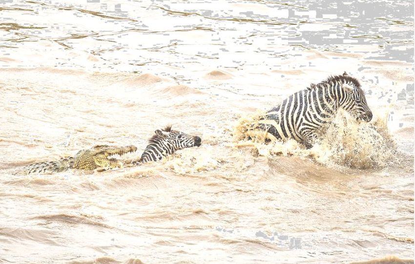
Under review as a conference paper at ICLR 2022

R EFERENCES
Abubakar Abid, Ali Abdalla, Ali Abid, Dawood Khan, Abdulrahman Alfozan, and James Zou.
  Gradio: Hassle-free sharing and testing of ml models in the wild. arXiv preprint arXiv:1906.02569,
  2019.
Julius Adebayo and Lalana Kagal. Iterative orthogonal feature projection for diagnosing bias in
  black-box models. arXiv preprint arXiv:1611.04967, 2016.
Julius Adebayo, Justin Gilmer, Michael Muelly, Ian J. Goodfellow, Moritz Hardt, and
  Been Kim. Sanity checks for saliency maps. In Samy Bengio, Hanna M. Wallach,
  Hugo Larochelle, Kristen Grauman, Nicolò Cesa-Bianchi, and Roman Garnett (eds.), Ad-
  vances in Neural Information Processing Systems 31: Annual Conference on Neural
  Information Processing Systems 2018, NeurIPS 2018, December 3-8, 2018, Montréal,
  Canada, 2018.    URL https://proceedings.neurips.cc/paper/2018/hash/
  294a8ed24b1ad22ec2e7efea049b8737-Abstract.html.
Ahmed Alqaraawi, M. Schuessler, Philipp Weiß, Enrico Costanza, and Nadia Bianchi-Berthouze.
  Evaluating saliency map explanations for convolutional neural networks: a user study. Proceedings
  of the 25th International Conference on Intelligent User Interfaces, 2020.
Aditya Chattopadhay, Anirban Sarkar, Prantik Howlader, and Vineeth N Balasubramanian. Grad-
  cam++: Generalized gradient-based visual explanations for deep convolutional networks. In 2018
 IEEE Winter Conference on Applications of Computer Vision (WACV), pp. 839–847, 2018. doi:
 10.1109/WACV.2018.00097.
Jia Deng, Wei Dong, Richard Socher, Li-Jia Li, Kai Li, and Li Fei-Fei. Imagenet: A large-scale hier-
   archical image database. In 2009 IEEE Conference on Computer Vision and Pattern Recognition,
   pp. 248–255, 2009. doi: 10.1109/CVPR.2009.5206848.
Greg d’Eon, Jason d’Eon, James R Wright, and Kevin Leyton-Brown. The spotlight: A general
  method for discovering systematic errors in deep learning models. arXiv preprint arXiv:2107.00758,
  2021.
Amit Dhurandhar, Pin-Yu Chen, Ronny Luss, Chun-Chen Tu, Paishun Ting, Karthikeyan Shanmugam,
 and Payel Das. Explanations based on the missing: Towards contrastive explanations with pertinent
 negatives. arXiv preprint arXiv:1802.07623, 2018.
Thomas B. Fitzpatrick. The Validity and Practicality of Sun-Reactive Skin Types I Through
  VI. Archives of Dermatology, 124(6):869–871, 06 1988. ISSN 0003-987X. doi: 10.1001/
  archderm.1988.01670060015008. URL https://doi.org/10.1001/archderm.1988.
  01670060015008.
Ruth Fong and Andrea Vedaldi. Net2vec: Quantifying and explaining how concepts are encoded by
  filters in deep neural networks. In Proceedings of the IEEE conference on computer vision and
  pattern recognition, pp. 8730–8738, 2018.
Amirata Ghorbani, James Wexler, James Zou, and Been Kim. Towards automatic concept-based
 explanations. arXiv preprint arXiv:1902.03129, 2019.
Yash Goyal, Ziyan Wu, Jan Ernst, Dhruv Batra, Devi Parikh, and Stefan Lee. Counterfactual
  visual explanations. In Kamalika Chaudhuri and Ruslan Salakhutdinov (eds.), Proceedings of the
  36th International Conference on Machine Learning, ICML 2019, 9-15 June 2019, Long Beach,
  California, USA, volume 97 of Proceedings of Machine Learning Research, pp. 2376–2384. PMLR,
  2019. URL http://proceedings.mlr.press/v97/goyal19a.html.
Matthew Groh, Caleb Harris, Luis Soenksen, Felix Lau, Rachel Han, Aerin Kim, Arash Koochek,
 and Omar Badri. Evaluating deep neural networks trained on clinical images in dermatology with
 the fitzpatrick 17k dataset. arXiv preprint arXiv:2104.09957, 2021.
Kaiming He, Xiangyu Zhang, Shaoqing Ren, and Jian Sun. Deep residual learning for image
  recognition. In Proceedings of the IEEE conference on computer vision and pattern recognition,
  pp. 770–778, 2016.

                                                10
Under review as a conference paper at ICLR 2022
Dan Hendrycks and Kevin Gimpel. A baseline for detecting misclassified and out-of-distribution
examples in neural networks. arXiv preprint arXiv:1610.02136, 2016.
Gao Huang, Zhuang Liu, Laurens Van Der Maaten, and Kilian Q Weinberger. Densely connected
convolutional networks. In Proceedings of the IEEE conference on computer vision and pattern
recognition, pp. 4700–4708, 2017.
Forrest N Iandola, Song Han, Matthew W Moskewicz, Khalid Ashraf, William J Dally, and Kurt
Keutzer. Squeezenet: Alexnet-level accuracy with 50x fewer parameters and¡ 0.5 mb model size.
arXiv preprint arXiv:1602.07360, 2016.
Jeremy Irvin, Pranav Rajpurkar, Michael Ko, Yifan Yu, Silviana Ciurea-Ilcus, Chris Chute, Henrik
Marklund, Behzad Haghgoo, Robyn Ball, Katie Shpanskaya, et al. Chexpert: A large chest
radiograph dataset with uncertainty labels and expert comparison. In Proceedings of the AAAI
conference on artificial intelligence, volume 33, pp. 590–597, 2019.
Douwe Kiela, Max Bartolo, Yixin Nie, Divyansh Kaushik, Atticus Geiger, Zhengxuan Wu, Bertie
Vidgen, Grusha Prasad, Amanpreet Singh, Pratik Ringshia, et al. Dynabench: Rethinking bench-
marking in nlp. arXiv preprint arXiv:2104.14337, 2021.
Been Kim, Martin Wattenberg, Justin Gilmer, Carrie Cai, James Wexler, Fernanda Viegas, et al.
Interpretability beyond feature attribution: Quantitative testing with concept activation vectors
(tcav). In International conference on machine learning, pp. 2668–2677. PMLR, 2018.
Michael P Kim, Amirata Ghorbani, and James Zou. Multiaccuracy: Black-box post-processing for
fairness in classification. In Proceedings of the 2019 AAAI/ACM Conference on AI, Ethics, and
Society, pp. 247–254, 2019.
Diederik P Kingma and Jimmy Ba. Adam: A method for stochastic optimization. arXiv preprint
arXiv:1412.6980, 2014.
Pang Wei Koh and Percy Liang. Understanding black-box predictions via influence functions. In
International Conference on Machine Learning, pp. 1885–1894. PMLR, 2017.
Pang Wei Koh, Shiori Sagawa, Henrik Marklund, Sang Michael Xie, Marvin Zhang, Akshay Bal-
subramani, Weihua Hu, Michihiro Yasunaga, Richard Lanas Phillips, Irena Gao, et al. Wilds: A
benchmark of in-the-wild distribution shifts. arXiv preprint arXiv:2012.07421, 2020.
Agostina J Larrazabal, Nicolás Nieto, Victoria Peterson, Diego H Milone, and Enzo Ferrante. Gender
imbalance in medical imaging datasets produces biased classifiers for computer-aided diagnosis.
Proceedings of the National Academy of Sciences, 117(23):12592–12594, 2020.
Weixin Liang and James Zou. Metadataset: A dataset of datasets for evaluating distribution shifts
and training conflicts. arXiv preprint, 2021.
Zachary Lipton, Yu-Xiang Wang, and Alexander Smola. Detecting and correcting for label shift with
black box predictors. In International conference on machine learning, pp. 3122–3130. PMLR,
2018.
Jie Lu, Anjin Liu, Fan Dong, Feng Gu, Joao Gama, and Guangquan Zhang. Learning under concept
drift: A review. IEEE Transactions on Knowledge and Data Engineering, 31(12):2346–2363,
2018.
Divyat Mahajan, Chenhao Tan, and Amit Sharma. Preserving causal constraints in counterfactual
explanations for machine learning classifiers. arXiv preprint arXiv:1912.03277, 2019.
Claudio Michaelis, Benjamin Mitzkus, Robert Geirhos, Evgenia Rusak, Oliver Bringmann, Alexan-
der S. Ecker, Matthias Bethge, and Wieland Brendel. Benchmarking robustness in object detection:
Autonomous driving when winter is coming. arXiv preprint arXiv:1907.07484, 2019.
Bret Nestor, Matthew BA McDermott, Willie Boag, Gabriela Berner, Tristan Naumann, Michael C
Hughes, Anna Goldenberg, and Marzyeh Ghassemi. Feature robustness in non-stationary health
records: caveats to deployable model performance in common clinical machine learning tasks. In
Machine Learning for Healthcare Conference, pp. 381–405. PMLR, 2019.
11Under review as a conference paper at ICLR 2022
Erdem Okur and Mehmet Turkan. A survey on automated melanoma detection. Engineering
Applications of Artificial Intelligence, 73:50–67, 2018.
Aditi Raghunathan, Jacob Steinhardt, and Percy Liang. Semidefinite relaxations for certifying
robustness to adversarial examples. arXiv preprint arXiv:1811.01057, 2018.
Veronica Rotemberg, Nicholas Kurtansky, Brigid Betz-Stablein, Liam Caffery, Emmanouil
Chousakos, Noel Codella, Marc Combalia, Stephen Dusza, Pascale Guitera, David Gutman,
et al. A patient-centric dataset of images and metadata for identifying melanomas using clinical
context. Scientific data, 8(1):1–8, 2021.
Laleh Seyyed-Kalantari, Guanxiong Liu, Matthew McDermott, Irene Y Chen, and Marzyeh Ghassemi.
Chexclusion: Fairness gaps in deep chest x-ray classifiers. In BIOCOMPUTING 2021: Proceedings
of the Pacific Symposium, pp. 232–243. World Scientific, 2020.
Karen Simonyan, Andrea Vedaldi, and Andrew Zisserman. Deep inside convolutional networks:
Visualising image classification models and saliency maps. arXiv preprint arXiv:1312.6034, 2013.
Krishna Kumar Singh, Dhruv Kumar Mahajan, Kristen Grauman, Yong Jae Lee, Matt Feiszli, and
Deepti Ghadiyaram. Don’t judge an object by its context: Learning to overcome contextual
bias. 2020 IEEE/CVF Conference on Computer Vision and Pattern Recognition (CVPR), pp.
11067–11075, 2020.
Sumedha Singla, Brian Pollack, Junxiang Chen, and Kayhan Batmanghelich. Explanation by
progressive exaggeration. In International Conference on Learning Representations, 2020. URL
https://openreview.net/forum?id=H1xFWgrFPS.
Adarsh Subbaswamy, Peter Schulam, and Suchi Saria. Preventing failures due to dataset shift:
Learning predictive models that transport. In The 22nd International Conference on Artificial
Intelligence and Statistics, pp. 3118–3127. PMLR, 2019.
Sahil Verma, John Dickerson, and Keegan Hines. Counterfactual explanations for machine learning:
A review. arXiv preprint arXiv:2010.10596, 2020.
Sandra Wachter, Brent Mittelstadt, and Chris Russell. Counterfactual explanations without opening
the black box: Automated decisions and the gdpr. Harv. JL & Tech., 31:841, 2017.
X Wang, Y Peng, L Lu, Z Lu, M Bagheri, and R Summers. Hospital-scale chest x-ray database and
benchmarks on weakly-supervised classification and localization of common thorax diseases. In
IEEE CVPR, volume 7, 2017.
James Wexler, Mahima Pushkarna, Tolga Bolukbasi, Martin Wattenberg, Fernanda Viégas, and Jimbo
Wilson. The what-if tool: Interactive probing of machine learning models. IEEE Transactions on
Visualization and Computer Graphics, 26(1):56–65, 2020. doi: 10.1109/TVCG.2019.2934619.
Eric Wu, Kevin Wu, Roxana Daneshjou, David Ouyang, Daniel E Ho, and James Zou. How medical
ai devices are evaluated: limitations and recommendations from an analysis of fda approvals.
Nature Medicine, 27(4):582–584, 2021.
Bolei Zhou, Aditya Khosla, Agata Lapedriza, Aude Oliva, and Antonio Torralba. Learning deep
features for discriminative localization. In Proceedings of the IEEE conference on computer vision
and pattern recognition, pp. 2921–2929, 2016.
Bolei Zhou, Yiyou Sun, David Bau, and Antonio Torralba. Interpretable basis decomposition for
visual explanation. In Proceedings of the European Conference on Computer Vision (ECCV), pp.
119–134, 2018.
12Under review as a conference paper at ICLR 2022
A A PPENDIX
A.1 L EARNING C ONCEPTS
Here we provide implementational details on how we learn the concept activation vectors (CAVs).
Concretely, we pick a bottleneck layer in our model, which is the representation space in which we
will learn our features. Unless otherwise stated, we choose the penultimate layer in ResNet18 for
experiments in this paper. Let m be the dimensionality of the bottleneck layer L, and bL : Rd → Rm
be the “bottom” of the network, which maps samples from the input space to the bottleneck layer,
and tL : Rm → Rk be the “top” of the network, defined analogously. In generating conceptual
explanations, the first step is to define a concept library: a set of human-interpretable concepts
C = {c1 , c2 , ...} that occur in the dataset. For each concept, we collect positive examples, Pci , that
exhibit the concept, as well as negative examples, Nci , in which the concept is absent. Then, we train
a support vector machine to classify {bL (x) : x ∈ Pci } from {bL (x) : x ∈ Nci }, the same way as
in Kim et al. (2018). Overall pseudocode for the procedure can be found in Figure 5.
Algorithm 2: Learning concept vectors
Inputs :
f # trained network: model
L # bottleneck layer (hyperparameter): int
concepts # set of concepts: set[str]
P # positive examples per concept: dict[str,
list[sample]]
N # negative examples per concept: dict[str,
list[sample]]
Return : svms #Set of SVMs containing concept predictors.
1 b, t = f.layers[:L], f.layers[L:] # Divide network f (·) into a
bottom b (first l layers) and top t (remaining layers) so that
f (·) = t(b(·))
2 for c in concepts: # Per concept, learn an SVM to classify
bottleneck representations of positive and negative examples.
3 svms[c] = svm.train(b(P[c]), b(N[c]))
4 # Filter out concepts that are not learned well (i.e.
validation accuracies below a particular threshold).
5 if svms[c].acc < .7:
6 del svms[c]
Figure 5: Pseudocode for CES in Python-like syntax concept learning procedure. Learning the
concepts (lines 1-6) just needs to be done once and can be carried out offline.
A.2 M ETA DATASET E XPERIMENTS
In Table 2, we provide results over 20 scenarios. In each of the scenarios, we fine-tune only the
classification layer of a ResNet18(He et al., 2016) pretrained on ImageNet, which outputs a probability
distribution over 5 animals(cat, dog, bear, bird, elephant). For instance, in the case of the dog(snow)
experiment, we train the model with images of dogs that are all taken with snow. We replicate this
experiment with 20 different animal & concept combinations and report the results below.
In Table 3, for each scenario, we sample 50 images with and without the concept and we report the
accuracy over those images. We observe a start difference between accuracies, which verifies that
model learns to rely on the correlation.
A.3 VALIDITY E XAMPLES
In Fig. 7, we provide additional examples on where validity improves explanations. In a) we have a
model trained with the dog-snow spurious correlation and in b) we have the dog class associated with
both the horse and bed concepts. For both of these examples, we observe that in the images where
13Under review as a conference paper at ICLR 2022
Experiment CCE-Prec.@3 CCE(Univariate)-Prec.@3 CCE(Control)-Prec.@3
dog(chair) 0.980 0.360 0
cat(cabinet) 1 1 0.180
dog(snow) 1 1 0
dog(car) 1 1 0
dog(horse) 1 1 0.500
bird(water) 0.960 1 0.660
dog(water) 0.980 0.980 0
dog(fence) 1 0.980 0
elephant(building) 1 0.821 0
cat(keyboard) 0.860 0.800 0
dog(sand) 0.760 0.900 0
cat(computer) 0.980 1 0
dog(bed) 1 1 0
cat(bed) 0.980 1 0
cat(book) 0.960 1 0
dog(grass) 0.700 0.780 0
cat(mirror) 0.900 0.900 0
bird(sand) 0.960 1 0
bear(chair) 0.940 0.720 0
cat(grass) 0.940 0.900 0
Table 2: Empirical evaluation for detecting spurious correlations in the training data. We report
results over 20 scenarios, where each class is associated with the concept in parenthesis during the
training phase.
Experiment Accuracy for Images with the Concept Accuracy for Images Without the Concept
dog(chair) 0.74 0.54
cat(cabinet) 0.8 0.62
dog(snow) 0.76 0.12
dog(car) 0.86 0.66
dog(horse) 0.70 0.36
bird(water) 0.78 0.42
dog(water) 0.82 0.4
dog(fence) 0.74 0.52
elephant(building) 0.82 0.72
cat(keyboard) 0.96 0.46
dog(sand) 0.66 0.42
cat(computer) 1.0 0.68
dog(bed) 0.86 0.46
cat(bed) 0.84 0.54
cat(book) 0.9 0.64
dog(grass) 0.96 0.56
cat(mirror) 0.86 0.4
bird(sand) 0.78 0.66
bear(chair) 0.82 0.44
cat(grass) 0.72 0.46
Table 3: Accuracy of the model for images tested with and without the confounding variable.
the proposed concept already exists, validity constraints help prevent the model from explaining the
mistake by adding that particular concept, which results in valid explanations.
14Under review as a conference paper at ICLR 2022
Input to Method
a
African hunting dog (66%)
African crocodile (42%)
Correct label → Zebra Correct label → Zebra
b
Stripes 1.00 Field 1.00
Cow 0.52 Cow 0.89
Dog –0.35 Stripes 0.87
Flag 0.20 Buildings 0.82
Polka dots –0.20 Water –0.79
Conceptual Counterfactuals
Figure 6: Different reasons of model mistakes for the same class..
a) Spurious Correlation: Dog(Snow) b) Spurious Correlation: Dog(Horse) & Dog(Bed)
Dog(Snow) Pred. Images Method Horse Bed
Pred: Bird (48%) Pred: Bear (47%)
Bear Univariate 3 2
(33%)
CCE(no 8 2
validity)
Full CCE 158 2
Cat
Univariate 1 3
(37%)
CCE(no 1 6
validity)
Method Rank of Method Rank of Full CCE 1 142
Snow Snow
Bird Univariate 1 2
Univariate 3 Univariate 1
(29%)
CCE(no validity) CCE(no validity) CCE(no 1 3
1 1
validity)
Full CCE 154 Full CCE 1 Full CCE 1 2
Figure 7: Validity constraint improves explanations. .
A.4 D ERMATOLOGY E XPERIMENT WITH F ITZPATRICK 17 K
We directly follow the experimental protocol in Groh et al. (2021). Fitzpatrick17k (Groh et al., 2021)
is a dermatology dataset that contains 16,577 skin images with 114 different skin conditions. For
15Under review as a conference paper at ICLR 2022
these images, skin type labels are provided using the Fitzpatrick system (Fitzpatrick, 1988). Groh
et al. (2021) decomposes the dataset into three groups: The lightest skin types (1 & 2) with 7,755
images, the middle skin types (3 & 4) with 6,089 images, the darkest skin types (5 & 6) with 2,168
images. We randomly partition the dataset into training(80%) and testing(20%) sets. We use a
ResNet18 (He et al., 2016) backbone pretrained on ImageNet(Deng et al., 2009) and we fine-tune
a classification head to predict one of the 114 skin conditions using Adam(Kingma & Ba, 2014)
optimizer. The classification head consists of 1) a fully-connected layer with 256 hidden units 2) relu
activation 3) dropout layer with a 40% probability of masking activations 4) another fully-connected
layer with the number of predicted categories. We obtain the training script from the repository1 for
the paper Groh et al. (2021).
We are using the imagecorruptions2 (Michaelis et al., 2019) library to obtain positive samples of
defocus blur(3), zoom blur(2), brightness(3), motion blur(3), and contrast(2), where we used the
severity levels provided in parenthesis. Examples of positive images for these concepts can be found
in Fig. 8.
We learn the zoom concept by cropping the height and width of images to a fourth of their sizes. We
obtain positive images from the darkest skin types (5&6) and negative images from the lightest skin
types (1&2) to learn the dark skin color concept. For all dermatology concepts except the skin hair
concept, we use 25 positive & negative pairs of images. For the skin hair concept, we use 10 pairs of
images from the ISIC dataset (Rotemberg et al., 2021).
A.4.1 E XPLANATION A RTIFACTS
It is important to note that sometimes concepts such as water or ashcan may be suggested as
explanations by CCE. Concepts are represented as vectors in the embedding space, and there may be
similarities among them. Hence, water or ashcan concepts may be very similar to certain textures
that are relevant to the dermatology task, where it was not possible to obtain the true concept itself.
The practitioner using CCE to explain the mistake can easily discard these artifacts suggested by
CCE, where there is also concepts that are more relevant and obtained larger scores. Secondly, as
the user keeps using concept-based methods, they can understand what type of concepts is needed,
or is relevant to the task. Accordingly, it is possible to update and obtain a more informative bank.
Generally, there are various interesting directions that could be pursued in the human-machine
interface that would improve the real-life performance of explanation algorithms. We are also
interested in further understanding this, and think more about the deployment aspects of CCE in
future work.
A.4.2 T ESTING G RAD CAM++ IN THE F ITZPATRICK S ETTING
As we mention in Section 4.4, the allergic contact dermatitis condition has a biased skin color
distribution in the training data. Activation-map-based methods such as GradCAM++(Chattopadhay
et al., 2018) fail to communicate this to the user. However, CCE can correctly identify this as a reason
why the model fails. In Figure 9 we show two examples where CCE is able to identify the bias in
the data that drives the model mistake; however, one of the methods that are very commonly used to
understand model predictions, GradCAM++, fails to identify this reason.
A.5 C ARDIOLOGY E XPERIMENT WITH C HEST X-R AYS
We investigate a cross-site evaluation setting, where models trained on Chest X-Ray images are used
to classify the pneumothorax condition which was proposed in (Wu et al., 2021). Using pretrained
models from (Wu et al., 2021), we use a DenseNet-121(Huang et al., 2017) architecture pretrained
on ImageNet(Deng et al., 2009) and then fine-tuned on the NIH dataset(Wang et al., 2017). As it is
reported in their paper, this model achieves 0.779 mean AUC when tested on the (Irvin et al., 2019)
dataset and 0.903 mean AUC when tested on the NIH dataset. We use CCE to explain mistake over a
subset of the SHC dataset. Specifically, we run CCE over the images taken from the lateral view,
which does not exist in the training dataset since NIH only contains images from the frontal (Anterior-
Posterior(AP) or Posterior-Anterior(PA)) view positions. This constitutes a real-life scenario of
1
https://github.com/mattgroh/fitzpatrick17k
2
https://github.com/bethgelab/imagecorruptions
16You can also read