The Landslide Velocity - Geo Uni Bonn
←
→
Page content transcription
If your browser does not render page correctly, please read the page content below
The Landslide Velocity

                                                                                   Shiva P. Pudasaini a,b , Michael Krautblatter a
                                                                          a Technical University of Munich, Chair of Landslide Research
                                                                                   Arcisstrasse 21, D-80333, Munich, Germany
                                                                        b University of Bonn, Institute of Geosciences, Geophysics Section
arXiv:2103.10939v1 [physics.geo-ph] 15 Mar 2021

                                                                               Meckenheimer Allee 176, D-53115, Bonn, Germany
                                                                                          E-mail: shiva.pudasaini@tum.de

                                                  Abstract: Proper knowledge of velocity is required in accurately determining the enormous destructive energy
                                                  carried by a landslide. We present the first, simple and physics-based general analytical landslide velocity model
                                                  that simultaneously incorporates the internal deformation (non-linear advection) and externally applied forces,
                                                  consisting of the net driving force and the viscous resistant. From the physical point of view, the model stands
                                                  as a novel class of non-linear advective − dissipative system where classical Voellmy and inviscid Burgers’
                                                  equation are specifications of this general model. We show that the non-linear advection and external forcing
                                                  fundamentally regulate the state of motion and deformation, which substantially enhances our understanding
                                                  of the velocity of a coherently deforming landslide. Since analytical solutions provide the fastest, the most cost-
                                                  effective and the best rigorous answer to the problem, we construct several new and general exact analytical
                                                  solutions. These solutions cover the wider spectrum of landslide velocity and directly reduce to the mass point
                                                  motion. New solutions bridge the existing gap between the negligibly deforming and geometrically massively
                                                  deforming landslides through their internal deformations. This provides a novel, rapid and consistent method
                                                  for efficient coupling of different types of mass transports. The mechanism of landslide advection, stretching and
                                                  approaching to the steady-state has been explained. We reveal the fact that shifting, up-lifting and stretching
                                                  of the velocity field stem from the forcing and non-linear advection. The intrinsic mechanism of our solution
                                                  describes the fascinating breaking wave and emergence of landslide folding. This happens collectively as the
                                                  solution system simultaneously introduces downslope propagation of the domain, velocity up-lift and non-linear
                                                  advection. We disclose the fact that the domain translation and stretching solely depends on the net driving
                                                  force, and along with advection, the viscous drag fully controls the shock wave generation, wave breaking,
                                                  folding, and also the velocity magnitude. This demonstrates that landslide dynamics are architectured by
                                                  advection and reigned by the system forcing. The analytically obtained velocities are close to observed values in
                                                  natural events. These solutions constitute a new foundation of landslide velocity in solving technical problems.
                                                  This provides the practitioners with the key information in instantly and accurately estimating the impact
                                                  force that is very important in delineating hazard zones and for the mitigation of landslide hazards.

                                                  1    Introduction
                                                  There are three methods to investigate and solve a scientific problem: laboratory or field data, numerical
                                                  simulations of governing complex physical-mathematical model equations, or exact analytical solutions of sim-
                                                  plified model equations. This is also the case for mass movements including extremely rapid flow-type landslide
                                                  processes such as debris avalanches (Pudasaini and Hutter, 2007). The dynamics of a landslide is primarily
                                                  controlled by the flow velocity. Estimation of the flow velocity is key for assessment of landslide hazards, design
                                                  of protective structures, mitigation measures and landuse planning (Tai et al., 2001; Pudasaini and Hutter,
                                                  2007; Johannesson et al., 2009; Christen et al., 2010; Dowling and Santi, 2014; Cui et al., 2015; Faug, 2015;
                                                  Kattel et al., 2018). Thus, a proper understanding of landslide velocity is a crucial requirement for an appro-
                                                  priate modelling of landslide impact force because the associated hazard is directly and strongly related to the
                                                  landslide velocity (Huggel et al., 2005; Evans et al., 2009; Dietrich and Krautblatter, 2019). So, the landslide
                                                  velocity is of great theoretical and practical interest for both scientists and engineers. However, the mechanical
                                                  controls of the evolving velocity, runout and impact energy of the landslide have not yet been understood well.

                                                                                                          1
Due to the complex terrain, infrequent occurrence, and very high time and cost demands of field measurements,
the available data on landslide dynamics are insufficient. Proper understanding and interpretation of the data
obtained from the field measurements are often challenging because of the very limited nature of the material
properties and the boundary conditions. Additionally, field data are often only available for single location
and determined as static data after events. Dynamic data are rare (de Haas et al., 2020). So, much of the
low resolution measurements are locally or discretely based on points in time and space (Berger et al., 2011;
Schürch et al., 2011; McCoy et al., 2012; Theule et al., 2015; Dietrich and Krautblatter, 2019). Therefore,
laboratory or field experiments (Iverson et al., 2011; Iverson, 2012; de Haas and van Woerkom, 2016; Lu et
al., 2016; Lanzoni et al., 2017, Li et al., 2017; Pilvar et al., 2019; Baselt et al., 2021) and theoretical modelling
(Le and Pitman, 2009; Iverson and Ouyang, 2015; Pudasaini and Mergili, 2019) remain the major source of
knowledge in landslides and debris flow dynamics. Recently, there has been a rapid increase in the numerical
modelling for mass transports (McDougall and Hungr, 2005; Medina et al., 2008; Pudasaini, 2012; Cascini et
al., 2014; Cuomo et al., 2016; Frank et al., 2015; Iverson and Ouyang, 2015; Mergili et al., 2020a,b; Pudasaini
and Mergili, 2019; Qiao et al., 2019; Liu et al. 2021). However, to certain degree, numerical simulations are
approximations of the physical-mathematical model equations.

Although numerical simulations may overcome the limitations in the measurements and facilitate for a more
complete understanding by investigating much wider aspects of the flow parameters, run-out and deposition,
the usefulness of such simulations are often evaluated empirically (Mergili et al., 2020a, 2020b). In contrast,
exact, analytical solutions (Faug et al., 2010; Pudasaini, 2011) can provide better insights into the complex flow
behaviors, mainly the velocity, and their consequences. Moreover, analytical and exact solutions to non-linear
model equations are necessary to elevate the accuracy of numerical solution methods (Chalfen and Niemiec,
1986; Pudasaini, 2011, 2016; Pudasaini et al., 2018). For this reason, here, we are mainly concerned in pre-
senting exact analytical solutions for the newly developed general landslide velocity model equation.

Since Voellmy’s pioneering work, several analytical models and their solutions have been presented in litera-
ture for mass movements including extremely rapid flow-type landslide processes, avalanches and debris flows
(Voellmy, 1955; Salm, 1966; Perla et al., 1980; McClung, 1983). However, on the one hand, all these solutions
are effectively simplified to the mass point or center of mass motion. None of the existing analytical velocity
models consider the advection or the internal deformation. On the other hand, the parameters involved in these
models only represent restricted physics of the landslide material and motion. Nevertheless, a full analytical
model that includes a wide range of essential physics of the mass movements incorporating important process of
internal deformation and motion is still lacking. This is required for the more accurate description of landslide
motion.

In the recent years, different analytical solutions have been presented for mass transports. These include sim-
ple and reduced analytical solutions for avalanches and debris flows (Pudasaini, 2011), two-phase flows (Ghosh
Hajra et al., 2017, 2018), landslide and avalanche mobility (Pudasaini and Miller, 2013; Parez and Aharonov,
2015), fluid flows in porous and debris materials (Pudasaini, 2016), flow depth profiles for mud flow (Di Cristo
et al., 2018), simulating the shape of a granular front down a rough incline (Saingier et al., 2016), the granular
monoclinal wave (Razis et al., 2018) and the mobility of submarine debris flows (Rui and Yin, 2019). However,
neither a more general landslide model as we have derived here, nor the solution for such a model exists in
literature.

This paper presents a novel non-linear advective - dissipative transport equation with quadratic source term as
a function of the state variable (the velocity) and their exact analytical solutions describing the landslide motion
down a slope. The source term represents the system forcing, containing the physical/mechanical parameters
and the landslide velocity. Our dynamical velocity equation largely extends the existing landslide models and
range of their validity. The new landslide velocity model and its analytical solutions are more general and
constitute the full description for velocities with wide range of applied forces and the internal deformation
associated with the spatial velocity gradient. In this form, and with respect to the underlying physics and
dynamics, the newly developed landslide velocity model covers both the classical Voellmy and inviscid Burgers
equation as special cases, but it also describes fundamentally novel and broad physical phenomena. Impor-

                                                         2
tantly, the new model unifies the Voellmy and inviscid Burgers’ models and extends them further.
It is a challenge to construct exact analytical solutions even for the simplified problems in mass transport
(Pudasaini, 2011, 2016; Di Cristo et al., 2018; Pudasaini et al., 2018). In its full form, this is also true for
the landslide velocity model developed here. In contrast to the existing models, such as Voellmy-type and
Burgers-type, the great complexity in solving the new model equation analytically derives from the simultane-
ous presence of the internal deformation (non-linear advection, inertia) and the quadratic source representing
externally applied forces (in terms of velocity, including physical parameters). However, here, we advance
further by constructing various analytical and exact solutions to the new general landslide velocity model by
applying different advanced mathematical techniques, including those presented in Nadjafikhah (2009) and
Montecinos (2015). We revealed several major novel dynamical aspects associated with the general landslide
velocity model and its solutions. We show that a number of important physical phenomena are captured by
the new solutions. Some special features of the new solutions are discussed in detail. This includes - landslide
propagation and stretching; wave generation and breaking; and landslide folding. We also observed that dif-
ferent methods consistently produce similar analytical solutions. This highlights the intrinsic characteristics
of the landslide motion described by our new model. As exact, analytical solutions disclose many new and
essential physics, the solutions derived in this paper may find applications in environmental, engineering and
industrial mass transport down slopes and channels.
2 Basic Balance Equation for Landslide Motion
2.1 Mass and momentum balance equations
A geometrically two-dimensional motion down a slope is considered. Let t be time, (x, z) be the coordinates
and (g x , gz ) the gravity accelerations along and perpendicular to the slope, respectively. Let, h and u be the
flow depth and the mean flow velocity along the slope. Similarly, γ, αs , µ be the density ratio between the fluid
and the particles (γ = ρf /ρs ), volume fraction of the solid particles (coarse and fine solid particles), and the
basal friction coefficient (µ = tan δ), where δ is the basal friction angle, in the mixture material. Furthermore,
K is the earth pressure coefficient as a function of internal and the basal friction angles, and CDV is the viscous
drag coefficient.
We start with the multi-phase mass flow model (Pudasaini and Mergili, 2019) and include the viscous drag
(Pudasaini and Fischer, 2020). For simplicity, we first assume that the relative velocity between coarse and
fine solid particles (us , uf s ) and the fluid phase (uf ) in the landslide (debris) material is negligible, that is,
us ≈ uf s ≈ uf =: u, and so is the viscous deformation of the fluid. This means, for simplicity, we are considering
an effectively single-phase mixture flow. Then, by summing up the mass and momentum balance equations,
we obtain a single mass and momentum balance equation describing the motion of a landslide as:
∂h ∂
+ (hu) = 0, (1)
∂t ∂x
" #
∂ ∂ h2 ∂h
(hu) + hu2 + (1 − γ) αs gz K = h gx − (1 − γ) αs gz µ − g z {1 − (1 − γ) αs } − CDV u2 , (2)
∂t ∂x 2 ∂x
where − (1 − αs ) g z ∂h/∂x emerges from the hydraulic pressure gradient associated with possible interstitial
fluids in the landslide. Moreover, the term containing K on the left hand side and the other terms on the
right hand side in the momentum equation (2) represent all the involved forces. The first term in the square
bracket on the left hand side of (2) describes the advection, while the second term (in the square bracket)
describes the extent of the local deformation that stems from the hydraulic pressure gradient of the free-
surface of the landslide. The first, second, third and fourth terms on the right hand side of (2) are the gravity
acceleration; effective Coulomb friction that includes lubrication (1 − γ), liquefaction (αs ) (because, if there
is no or substantially low amount of solid, the mass is fully liquefied, e.g., lahar flows); the local deformation
due to the pressure gradient; and the viscous drag, respectively. Note that the term with 1 − γ or γ originates
3from the buoyancy effect. By setting γ = 0 and αs = 1, we obtain a dry landslide, grain flow or an avalanche
motion. For this choice, the third term on the right hand side vanishes. However, we keep γ and αs also to
include possible fluid effects in the landslide (mixture).
2.2 The landslide velocity equation
The momentum balance equation (2) can be re-written as:
∂u ∂u ∂h ∂
h +u +u + (hu)
∂t ∂x ∂t ∂x
∂h
= h gx –(1 − γ)αs gz µ–gz {((1 − γ) K + γ) αs + (1 − αs )} − CDV u2 . (3)
∂x
Note that for K = 1 (which mostly prevails for extensional flows, Pudasaini and Hutter, 2007), the third term
on the right hand side associated with ∂h/∂x simplifies drastically, because {((1 − γ) K + γ) αs + (1 − αs )}
becomes unity. So, the isotropic assumption (i.e., K = 1) loses some important information about the solid
content and the buoyancy effect in the mixture. Employing the mass balance equation (1), the momentum
balance equation (3) can be re-written as:
∂u ∂u ∂h
+u = gx –(1 − γ)αs gz µ–gz {((1 − γ) K + γ) αs + (1 − αs )} − CDV u2 . (4)
∂t ∂x ∂x
The gradient ∂h/∂x might be approximated, say as hg , and still include its effect as a parameter that may be
estimated. Here, we are mainly interested in developing a simple but more general landslide velocity model
than the existing ones that can be solved analytically and highlight its essence to enhance our understanding
of the landslide dynamics.
Now, with the notation α := g x –(1 − γ)αs gz µ–gz {((1 − γ) K + γ) αs + (1 − αs )} hg , which includes the forces:
gravity; friction, lubrication and liquefaction; and surface gradient; and β := CDV , which is the viscous drag
coefficient, (4) becomes a simple model equation:
∂u ∂u
+u = α − βu2 , (5)
∂t ∂x
where α and β constitute the net driving and the resisting forces in the system. We call (5) the landslide
velocity equation.
2.3 A novel physical−mathematical system
Equation (5) constitutes a genuinely novel class of non-linear advective - dissipative system and involves dynamic
interactions between the non-linear advective (or, inertial) term u∂u/∂x and the external forcing (source) term
α − βu2 . However, in contrast to the viscous Burgers’ equation where the dissipation is associated with the
(viscous) diffusion, here, dissipation stems because of the viscous drag, −βu2 . In the form, (5) is similar to the
classical shallow water equation. However, from the mechanics and the material composition, it is much wider
as such model does not exit in literature. From the physical and mathematical point of view, there are two
crucial novel aspects associated with the model (5). First, it explains the dynamics of deforming landslide and
thus extends the classical Voellmy model (Voellmy, 1955; Salm, 1966; McClung, 1983; Pudasaini and Hutter,
2007) due to the broad physics carried by the model parameters, α, β; and the dynamics described by the new
term u∂u/∂x. These parameters and the term u∂u/∂x control the landslide deformation and motion. Second,
it extends the classical non-linear inviscid Burgers’ equation by including the non-linear source term, α − βu2 ,
as a quadratic function of the unknown field variable, u, taking into account many different forces associated
with the system as explained in Section 2.2.
From the structure, (5) is a fundamental non-linear partial differential equation, or a non-linear transport
equation with a source, where the source is the external physical forcing. Such equation explains the non-linear
advection with source term that contains the physics of the underlying problem through the parameters α and
4β. The form of this equation is very important as it may describe the dynamical state of many extended (as
compared to the Voellmy and Burgers models) physical and engineering problems appearing in nature, science
and technology, including viscous/fluid flow, traffic flow, shock theory, gas dynamics, landslide and avalanches
(Burgers, 1948; Hopf, 1950; Cole, 1951; Nadjafikhah, 2009; Pudasaini, 2011; Montecinos, 2015).
3 The Landslide Velocity: Simple Solutions
Exact analytical solutions to simplified cases of non-linear debris avalanche model equations are necessary to
calibrate numerical simulations of flow depth and velocity profiles. These problem-specific solutions provide
important insight into the full behavior of the system. Physically meaningful exact solutions explain the true
and entire nature of the problem associated with the model equation, and thus, are superior over numerical
simulations (Pudasaini, 2011; Faug, 2015).
One of the main purposes of this contribution is to obtain exact analytical velocities for the landslide model (5).
In the form (5) is simple. So, one may tempt to solve it analytically to explicitly obtain the landslide velocity.
However, it poses a great mathematical challenge to derive explicit analytical solutions for the landslide velocity,
u. This is mainly due to the new terms appearing in (5). Below, we construct five different exact analytical
solutions to the model (5) in explicit form. In order to gain some physical insights into the landslide motion, the
solutions are compared to each other. Equation (5) can be considered in two different ways: steady-state and
transient motions, and both without and with (internal) deformation that is described by the term u∂u/∂x.
3.1 Steady−state motion
For a sufficiently long time and sufficiently long slope, the time independent steady-state motion can be devel-
oped. Then, (5) reduces to a simplified equation for the landslide velocity down the entire slope:
∂ 1 2
u = α − βu2 . (6)
∂x 2
Equivalently, this also represents a mass point velocity along the slope. Classically, (6) is called the center of
mass velocity of a dry avalanche of flow type (Perla et al., 1980).
3.1.1 Negligible viscous drag
In situations when the Coulomb friction is dominant and the motion is slow, the viscous drag contribution can
be neglected (βu2 ≈ 0), e.g., typically the moment after the mass release. Then, the solution to (6) is given by
(Solution A): q
u(x; α) = 2α (x − x0 ) + u20 , (7)
where x is the downslope travel distance, and u0 is the initial velocity at x0 (or, a boundary condition). Solution
(7) recovers the landslide velocity obtained by considering the simple energy balance for a mass point in which
only the gravity and simple dry Coulomb frictional forces are considered (Scheidegger, 1973), both of these
forces are included in α. Furthermore, when the slope angle is sufficiently high or close to vertical, (7) also
represents a near free fall landslide or rockfall velocity for which x changes to the vertical height drop.
3.1.2 Viscous drag included
In general, depending on the magnitude of the net driving force (that also includes the Coulomb friction), the
viscous drag and the magnitude of the velocity, either α or βu2 , or both can play dominant role in determining
the landslide motion. Then, the more general solution for (6) than (7) takes the form (Solution B):
s
α β 1
u(x; α, β) = 1 − 1 − u20 , (8)
β α exp(2β(x − x0 ))
5150
Velocity: u [ms-1]
100
50
Without viscous drag
With viscous drag
0
0 500 1000 1500
Travel distance: x [m]
Figure 1: The landslide velocity distributions down the slope as a function of position, for both without and
with drag given by (7) and (8), respectively. With drag, the flow attains the terminal velocity uT x ≈ 60.1 ms−1
at about x = 600 m, but without drag, the flow velocity increases unboundedly.
where, u0 is the initial velocity at x0 . The velocity given by (8) can be compared to the Voellmy velocity and
be used to calculate the speed of an avalanche (Voellmy, 1955; McClung, 1983). However, the Voellmy model
only considers the reduced physical aspects in which α merely includes the gravitational force due to the slope
and the dry Coulomb frictional force. This has been discussed in more detail in Section 3.2. As in (7), the
solution (8) can also represent a near free fall landslide (or rockfall) velocity when the slope angle is sufficiently
high or close to vertical, but now, it also includes the influence of drag, akin to the sky-jump.
It is important to reveal the dynamics of viscous drag in the landslide motion. The major aspect of viscous
drag is to bring the velocity (motion) to a terminal velocity (steady, uniform) for a sufficiently long travel
distance. This is achieved by the following relation obtained from (8):
α
r
lim u = =: uT x , (9)
x→∞ β
where uT x stands for the terminal velocity of a deformable mass, or a mass point motion (Voellmy), along the
slope that is often used to calculate the maximum velocity of an avalanche (Voellmy, 1955; McClung, 1983;
Pudasaini and Hutter, 2007).
In what follows, unless otherwise stated, we use the plausibly chosen physical parameters for rapid mass
movements: slope angle of about 50◦ , γ = 1100/2700, αs = 0.65, δ = 20◦ (Mergili et al., 2020a, 2020b;
Pudasaini and Fischer, 2020). This implies the model parameters α = 7.0, β = 0.0019. In reality, based
on the physics of the material and the flow, the numerical values of these model parameters should be set
appropriately. However, in principle, all the results presented here are valid for any choice of the parameter
set {α, β}. For simplicity, u0 = 0 is set at x0 = 0, which corresponds to initially zero velocity at the position
of the mass release. Figure 1 displays the velocity distributions of a landslide down the slope as a function
of the slope position x. The magnitudes of the solutions presented here are mainly for the reference purpose,
which, however, are subject to scrutiny with laboratory or field data as well as natural events. For the order of
magnitudes of velocities of natural events, we refer to Section 3.2.2. The velocities in Fig. 1 with and without
drag, equations (7) and (8), respectively, behave completely differently already after the mass has moved a
certain distance. The difference
p increases rapidly as the mass slides further down the slope. With the drag,
the terminal velocity (uT x = α/β ≈ 60.1 ms−1 ) is attained at a sufficient distance (about x = 600 m). But,
without drag, the velocity increases forever which is less likely for a mass propagating down a long distance.
6We note that as β → 0, the solution (8) approaches (7). For relatively small travel distance, say x ≤ 50 m,
these two solutions are quite similar as the viscous drag is not sufficiently effective yet. However, for a long
travel distance, x ≫ 50 m, when the viscous drag in not included, the landslide velocity increases steadily
without any control, whilst it increases only slowly, and remains almost unchanged for x ≥ 500 m when the
viscous drag effect is involved.
3.2 A mass point motion
Assume no or negligible local deformation (e.g., ∂u/∂x ≈ 0), or a Lagrangian description. Both are equivalent
to the mass point motion. In this situation, only the ordinary differentiation with respect to time is involved,
and ∂u/∂t can be replaced by du/dt. Then, the model (5) reduces to
du
= α − βu2 . (10)
dt
Perla et al. (1980) also called (10) the governing equation for the center of mass velocity, however, for a dry
avalanche of flow type. This is a simple non-linear first order ordinary differential equation. This equation
can be solved to obtain exact analytical solution for velocity of the landslide motion in terms of a tangent
hyperbolic function (Solution C):
s
α β
r p
u(t; α, β) = tanh αβ (t − t0 ) + tanh−1 u0 , (11)
β α
where, u0 = u (t0 ) is the initial velocity at time t = t0 . Equation (11) provides the time evolution of the velocity
of the coherent (without fragmentation and deformation) sliding mass until the time it fragments and/or moves
like an avalanche. This transition time is denoted by tA (or, tF ) indicating fragmentation, or the inception of
the avalanche motion due to fragmentation or large deformation. So, (11) is valid for t < tA . For t > tA , we
must use the full dynamical mass flow model (Pudasaini, 2012; Pudasaini and Mergili, 2019), or the equations
(1) and (2). For more detail on it, see Section 6.1.
For sufficiently long time, or in the limit, as the viscous force brings the motion to a non-accelerating state
(steady, uniform), from (11) we obtain:
α
r
lim u = =: uT t , (12)
t→∞ β
where uT t stands for the terminal velocity of the motion of a point mass.
The landslide position: Since u(t) = dx/dt, (11) can be integrated to obtain the landslide position as a
function of time:
s s
1 p β 1 β
x(t; α, β) = x0 + ln cosh αβ (t − t0 ) − tanh−1 u0 − ln cosh − tanh−1 u0 , (13)
β α β α
where x0 corresponds to the position at the initial time t0 .
Figure 2 displays the velocity profile of a landslide down the slope as a function of the time as given by (11).
For simplicity, u0 = 0 is set as initial condition at
t0 = 0,pwhich
corresponds to initially zero velocity at the time
of the landslide trigger. The terminal velocity uT t = α/β is attained at a sufficiently long time (∼ 15 s).
We note that, in the structure, the model (10) and its solution (11) exists in literature (Pudasaini and Hutter,
2007) and is classically called Voellmy’s mass point model (Voellmy, 1955), or Voellmy-Salm model (Salm,
1966) that disregards the position dependency of the landslide velocity (Gruber, 1989). But, (1 − γ), αs , and
the term associated with hg are new contributions and were not included in the Voellmy model, and K = 1
therein, while in our consideration α, K can be chosen appropriately. Thus, the Voellmy model corresponds to
the substantially reduced form of α, with α = gx − gz µ.
770
60
50
Velocity: u [ms-1]
40
30
20
10
0
0 5 10 15 20 25 30 35
Travel time: t [s]
Figure 2: Time evolution of the landslide velocity down the slope with drag given by (11). The motion attains
the terminal velocity at about t = 15 s.
3.2.1 The dynamics controlled by the physical and mechanical parameters
Solutions (8) and (11) are constructed independently, one for the velocity of a deformable mass as a function
of travel distance, or the velocity of the center of mass of the landslide down the slope, and the other for the
velocity of a mass point motion as a function of time. Unquestionable, they have their own dynamics. However,
for sufficiently long distance and sufficiently long time, or in the space and time limits, these solutions coincide
and we obtain a unique relationship:
α
r
uT x = uT t = . (14)
β
So, after a sufficiently long distance or a sufficiently long time, the forces
p associated with α and β always
maintain a balance resulting in the terminal velocity of the system, α/β. This is a fantastic situation.
Intuitively this is clear because, one could simply imagine that sufficiently long distance could somehow be
perceived as sufficiently long time, and for these limiting (but fundamentally different) situations, there exists
a single representative velocity that characterizes the dynamics. This has exactly happened, and is an advanced
understanding. This has been shown in Fig. 3 which implicitly indicates the equivalence between (8) and (11).
In fact, this can be proven, because, for the mass point or the center of mass motion,
du du dx du du 1 2 ∂u 1 2
= =u = u = u , (15)
dt dx dt dx dx 2 ∂x 2
is satisfied.
In Fig. 3, both velocities have the same limiting values, but their early behaviours are quite different. In space,
the velocity shows hyper increase after the incipient motion. However,pthe time evolution of velocity is slow
(almost linear) at first, then fast, and finally attains the steady-state, α/β = 60.1 ms−1 , the common value
for both the solutions.
3.2.2 The velocity magnitudes
Importantly, for a uniformly inclined slope, the landslide reaches its maximum or the terminal velocity after a
relatively short travel distance, or time with value on the order of 50 ms−1 . These are often observed scenarios,
e.g., for snow or rock-ice avalanches (Schaerer, 1975; Gubler, 1989; Christen et al., 2002; Havens et al., 2014).
The velocity magnitudes presented above are quite reasonable for fast to rapid landslides and debris avalanches
and correspond to several natural events (Highland and Bobrowsky, 2008). The front of the 2017 Piz-Chengalo
870
60
50
Velocity: u [ms-1]
40
30
20
10
0
0 500 1000 1500
Travel distance: x [m]
70
60
50
Velocity: u [ms-1]
40
30
20
10
0
0 5 10 15 20 25 30 35
Travel time: t [s]
Figure 3: Evolution of the landslide velocity down the slope as a function of space (top) given by (8), and
time (bottom) given by (11), respectively, both with drag. The flow attains the terminal velocity at about
x = 600 m and t = 15 s.
Bondo landslide (Switzerland) moved with more than 25 ms−1 already after 20 s of the rock avalanche release
(Mergili et al., 2020b), and later it moved at about 50 ms−1 (Walter et al., 2020). The 1970 rock-ice avalanche
event in Nevado Huascaran (Peru) reached mean velocity of 50 - 85 ms−1 at about 20 s, but the maximum
velocity in the initial stage of the movement reached as high as 125 ms−1 (Erismann and Abele, 2001; Evans et
al., 2009; Mergili et al. 2018). The 2002 Kolka glacier rock-ice avalanche in the Russian Kaucasus accelerated
with the velocity of about 60 - 80 ms−1 , but also attained the velocity as high as 100 ms−1 , mainly after the
incipient motion (Huggel et al., 2005; Evans et al., 2009).
3.2.3 Accelerating and decelerating motions
Depending on the magnitudes of the involved forces, and whether the initial mass was released or triggered
with a small (including zero) velocity or with high velocity, e.g., by a strong seismic shacking, (11) provides
fundamentally
p different but, physically meaningful velocity profiles. Both solutions asymptotically
p approach
α/β, the lead magnitude
p in (11). For notational convenience, we write S n (α, β) = α/β, which has the
dimension of velocity, α/β and is called the separation number (velocity) as it separates accelerating and
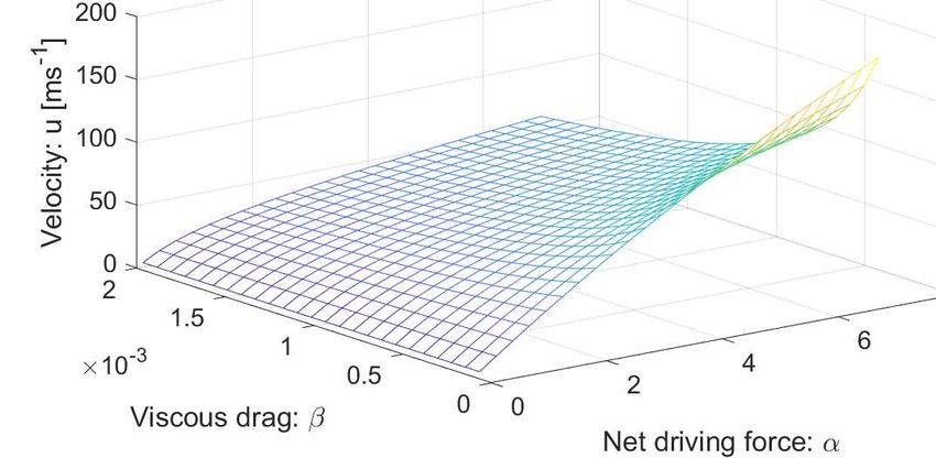
9Figure 4: The influence of the model parameters α and β on the landslide velocity. Colorbar shows velocity
distributions in ms−1 .
decelerating regimes. Description for deceleration has been given below. Furthermore, Sn includes all the
involved forces in the system and is the function of the ratio between the mechanically known forces: gravity,
friction, lubrication and surface gradient; and the viscous drag force. Thus, Sn fully governs the ultimate state
of the landslide motion.
For initial velocity less than Sn , i.e., u0 < Sn , the landslide velocity increases rapidly just after its release,
then ultimately (after a sufficiently long time) it approaches asymptotically to the steady state, Sn (Fig. 2).
This is the accelerating motion. On the other hand, if the initial velocity was higher than Sn , i.e., u0 > Sn ,
the landslide velocity would decrease rapidly just after its release, then it ultimately would asymptotically
approaches to Sn . This is the decelerating motion (not shown here).
We have now two possibilities. First, we can describe u(t; α, β) as a function of time with α, β as parameters.
This corresponds to the velocity profile of the particular landslide characterized by the geometrical, physical
and mechanical parameters α and β as time evolves. This has been shown in Fig. 2 for u0 < Sn . A similar
solution can be displayed for u0 > Sn for which the velocity would decrease and asymptotically approach to
Sn .
3.2.4 Velocity described by the space of physical parameters
Second, we can investigate the control of the physical parameters on the landslide motion for a given time. This
is achieved by plotting u(α, β; t) as a function of α and β, and considering time as a parameter. Figure 4 shows
the influence of the parameters α and β on the evolution of the velocity for a landslide motion for a typical
time t = 35 s. The parameters α and β enhance or control the landslide velocity completely differently. For a
set of parameters {α, β}, we can now provide an estimate of the landslide velocity. As mentioned earlier, the
landslide velocity as high as 125 ms−1 have been reported in the literature with their mean and common values
in the range of 60 - 80 ms−1 for rapid motions. This way, we can explicitly study the influence of the physical
parameters on the dynamics of the velocity field and also determine their range of plausible values. This
answers the question on how would the two similar looking, but physically differently characterized landslides
move. They may behave completely differently.
103.2.5 A model for viscous drag
There exists explicit models for the interfacial drags between the particles and the fluid (Pudasaini, 2020)
in the multiphase mixture flow (Pudasaini and Mergili, 2019). However, there exists no clear representation
of the viscous drag coefficient for landslide which is the drag between the landslide and the environment.
Often in applications, the drag coefficient (β = CDV ) is prescribed and is later calibrated with the numerical
simulations to fit with the observation or data (Kattel et al., 2016; Mergili et al., 2020a, 2020b). Here, we
explore an opportunity to investigate on how the characteristic landslide velocity (14) offers a unique possibility
to define the drag coefficient. Equation (14) can be written as
α
β= , (16)
u2max
where, umax represents the maximum possible velocity during the motion as obtained from the (long-time)
steady-state behaviour of the landslide. Equation (16) provides a clear and novel definition (representation) of
the viscous drag in mass movement (flow) as the ratio of the applied forces to the square of the steady-state
(or a maximum possible) velocity the system can attain. With the representative mass m, (16) can be written
as
1
mα
β= 12 2 . (17)
2 mumax
Equivalently, β is the ratio between the one half of the “system-force”, 21 mα (the driving force), and the
(maximum) kinetic energy, 12 mu2max , of the landslide. With the knowledge of the relevant maximum kinetic
energy of the landslide (Körner, 1980), the model (17) for the drag can be closed.
3.2.6 Landslide motion down the entire slope
Furthermore, we note that following the classical method by Voellmy (Voellmy, 1955) and extensions by Salm
(1966) and McClung (1983), the velocity models (8) and (11) can be used for multiple slope segments to
describe the accelerating and decelerating motions as well as the landslide run-out. These are also called the
release, track and run-out segments of the landslide, or avalanche (Gubler, 1989). However, for the gentle slope,
or the run-out, the frictional force may dominate gravity. In this situation, the sign of α in (5) changes. Then,
all the solutions derived above must be thoroughly re-visited with the initial condition for velocity being that
obtained from the lower end of the upstream segment. This way, we can apply the model (5) to analytically
describe the landslide motion for the entire slope, from its release, through the track and the run-out, as well
as to calculate the total travel distance. These methods can also be applied to the general solutions derived in
Section 4 and Section 5.
4 The Landslide Velocity: General Solution - I
For shallow motion the velocity may change locally, but the change in the landslide geometry may be param-
eterized. In such a situation, the force produced by the free-surface pressure gradient can be estimated. A
particular situation is the moving slab for which hg = 0, otherwise hg 6= 0. This justifies the physical signifi-
cance of (5).
The Lagrangian description of a landslide motion is easier. However, the Eulerian description provides a bet-
ter and more detailed picture of the landslide motion as it also includes the local deformation due to the
velocity gradient. So, here we consider the model equation (5). Without reduction, conceptually, this can
be viewed as an inviscid, non-homogeneous, dissipative Burgers’ equation with a quadratic source of system
forces, and includes both the time and space dependencies of u. Exact analytical solutions for (5) can still
be constructed, however, in more sophisticated forms, and is very demanding mathematically. First, for the
notational convenience, we re-write (5) as:
∂u ∂u
+ g(u) = f (u), (18)
∂t ∂x
11where, g(u) = u, and f (u) = α − βu2 correspond to our model (5). Here, g and f are sufficiently smooth
functions of u, the landslide velocity. Next, we construct exact analytical solution to the generic model (18).
For this, first we state the following theorem from Nadjafikhah (2009).
Theorem Z 4.1: Let f and g be invertible real valued functions of real variables, f is everywhere away from zero,
1 R
φ(u) = du is invertible, and l(u) = g φ−1 (u) du. Then, x = l(φ(u)) + F [t − φ(u)] is the solution
f (u)
of (18), where F is an arbitrary real valued smooth function of t − φ(u).
To our problem (5), we have constructed the solution (below in Section 4.1), and reads as (Solution D):
"p #
1 h p i 1 1 α/β + u
x = ln cosh αβ φ(u) + F [t − φ(u)] ; φ(u) = √ ln p . (19)
β 2 αβ α/β − u
It is important to note, that in (19), the major role is played by the function φ that contains all the forces of
the system. Furthermore, the function F includes the time-dependency of the solution. The amazing fact with
the solution (19) is that any smooth function F with its argument (t − φ(u)) is a valid solution of the model
equation. This means that, different landslides may be described by different F functions. Alternatively, a
class of landslides might be represented by a particular function F . This is a fundamentally great situation.
4.1 Derivation of the solution to the general model equation
Here, we present the detailed derivation of the solution (19) to the landslide velocity equation (5). We derive
the functions φ, φ−1 , l and loφ that are involved in constructing the analytical solution in Theorem 4.1 for our
model (5). The first function φ is given by
"p #
1 1 1 α/β + u
Z Z
φ(u) = du = 2
du = √ ln p . (20)
f (u) α − βu 2 αβ α/β − u
With the substitution, τ = φ(u) (which implies u = φ−1 (τ )), we obtain,
r " √ # r
−1 α exp 2 αβ τ − 1 α p
φ (τ ) = √ = tanh αβ τ . (21)
β exp 2 αβ τ + 1 β
So, now the second function φ−1 can be written in terms of u. However, √ we must
p be consistent with the physical
dimensions of the involved variables and functions. The quantities u, αβ, α/β and τ have dimensions of
ms−1 , s−1 , ms−1 and s. Thus, for the dimensional consistency, the following mapping introduces a new multiplier
λ with the dimension of 1/ ms−2 . Therefore, we have
α
r p
φ−1 (u) = tanh λαβ u . (22)
β
With this, the third function l(u) yields:
α 1
Z Z r Z p h p i
l(u) = g φ−1 (u) du = φ−1 (u) du = tanh λαβ u du = ln cosh λ αβ u . (23)
β λβ
The fourth function l (φ (u)) = (loφ)(u) is instantly achieved:
χ 1 h
p i
l (φ (u)) = ln cosh (ξλ) αβ φ(u) , (24)
λ β
where, as before, the multipliers χ and ξ emerge due to the transformation and for the dimensional consistency,
they have the dimensions of 1/ms−2 and ms−2 , respectively. The nice thing about the groupings (χ/λ) and
(ξλ) is that they are now dimensionless and unity.
Utilizing these functions in Theorem 4.1, we finally constructed the exact analytical solution (19) to the model
equation (5) describing the temporal and spatial evolution of the landslide velocity.
124.2 Recovering the mass point motion
The amazing fact is that the newly constructed general analytical solution (19) is strong and includes both
the mass point solutions for velocity (11) and the position (13). Below we prove, that for a special choice of
the function F , (19) directly implies both (11) and (13). For this, consider a particular form of F such that
F (0) ≡ 0, which is called a vacuum solution. First, F (0) ≡ 0 implies that t = φ(u). Then, with the functional
relation of φ(u) in (19), and after some simple algebraic operations, we obtain:
α
r hp i
u= tanh αβ t . (25)
β
Up to the constant of integration parameters (with u0 = 0 at t0 = 0), (25) is (11). So, the first assertion is
proved. Second, using F (0) ≡ 0 and φ(u) = t in (19), immediately yields
1 h p i
x= ln cosh αβ t . (26)
β
Again, up to the constant of integration parameters (with x0 = 0, and u0 = 0 at t0 = 0), (26) is (13). This
proves the second assertion.
Moreover, we mention that (25) and (26) can also be obtained formally proving that the conditions used on F
are legitimate. To see this, we differentiate (19) with respect to t to yield
dx α i dφ dφ
r hp
u= = tanh αβ φ(u) + F ′ [t − φ(u)] 1 − . (27)
dt β dt dt
But, differentiating φ in (19) with respect to t and employing (10), we obtain dφ/dt = 1, or φ = t. Now, by
substituting these in (27) and (19) we respectively recover (25) and (26).
However, we note that F in (19) is a general function. So, (19) provides a wide spectrum of analytical solutions
for the landslide velocity as a function of time and space, much wider than (11) and (13).
4.3 Some particular exact solutions
Here, we present some interesting particular exact solutions of (19) in the limit as β → 0. For this purpose,
first we consider (5) with β → 0, and introduce the new variables t̃ = αt, x̃ = αx. Then, (5) can be written as:
∂u ∂u
+u = 1. (28)
∂ t̃ ∂ x̃
Note that each term in this equation is dimensionless. We apply Theorem 4.1 and the underlying techniques to
(28). So, f (u) = 1 implies φ(u) = u, l(u) = u2 /2, and l(φ(u)) = u2 /2. Following the procedure as for (19), we
u2
obtain the solution to (28) as: x̃ = + F t̃ − u . However, the direct application of φ(u) = u in (19) leads
2
1 h p i
to the solution (that is more complex in its form): x̃ = ln cosh βu + F t̃ − u . Then, in the limit, we
β
must have:
1 h p i u2
lim ln cosh βu = . (29)
β→0 β 2
This is an important mathematical identity we obtained as a direct consequence of Theorem 4.1 and (19).
Furthermore, the identity (29) when applied to (26) implies:
1 h p i 1 h np √ oi 1 2
lim x = lim ln cosh αβ t = lim ln cosh β αt = αt . (30)
β→0 β→0 β β→0 β 2
Thus, x = 21 αt2 , which is the travel distance in time when the viscous drag is absent. So, (29) is a physically
important identity.
1370
60
Velocity: u [ms-1] 50
40
30
0 50 100 150 200 250 300 350 400
Travel distance: x [m]
Figure 5: Velocity distribution given by (34).
u2
Moreover, with the definition of x̃, for the particular choice of F ≡ 0, x̃ = + F t̃ − u results in u(x; α) =
√ 2
2αx, which
√ is the solution given in (7). Furthermore, with the choice of x̃ = 0, and F = t̃ − u, we obtain
u = 1 − 1 − 2αt, which for small t, can be approximated as u ≈ αt. But, in the limit as β → 0, (11) brings
about u = αt, which however, is valid for all t values. Thus, (19) generalizes both solutions (7) and (11) in
numerous ways.
4.4 Reduction to the classical Burgers’ equation
Interestingly, by directly taking limit as β → 0, from (19) we obtain
u2 u
x= +F t− , (31)
2α α
which can be written as
u
u2 + 2α F t − − 2α x = 0. (32)
α
Importantly, for any choice of the function F , (32) satisfies
∂u ∂u
+u = α, (33)
∂t ∂x
which reduces to the classical inviscid Burgers’ equation when α → 0.
4.5 Some explicit expressions for u in (19)
For a properly selected function F , (19) can be solved exactly for u. For example, consider a constant F ,
F = Λ. Then, an explicit exact solution is obtained as:
α 1
r n o
u= tanh exp 2 cosh−1 (exp(β(x − Λ))) . (34)
β 2
Figure 5 shows the velocity distribution given by (34) with u ≈ 28 ms−1 at x = 0 and Λ = 0, which reaches
the steady-state at about x = 150 m, much faster than the solution given by (8) in Fig. 3.
However, other more general solutions could be found by considering different F functions in (19). One such
1470
60
50
Velocity: u [ms-1]
40
30
20
10 Mass point velocity
General velocity
0
0 500 1000 1500
Travel distance: x [m]
Figure 6: Evolution of the velocity field along the slope as given by (35) for general velocity against the mass
point (or, center of mass) velocity corresponding to (8).
1 h np oi
case is presented here. For the choice F = ln c cosh αβ(t − φ(u)) , where c is a constant, (19) can be
β
solved explicitly for u in terms of x and t, which, after a lengthy algebra, takes the form:
α 1 2
r p p
u= tanh cosh−1 exp(βx) − cosh αβ t + αβ t . (35)
β 2 c
The velocity profile along the slope as given by (35) is presented in Fig. 6 for t = 1 ms−1 and c = 1. This
solution is quite different than that in Fig. 3 produced by (8) which does not consider the local time variation
of the velocity. From the dynamical perspective, the solution (35) is better than the mass point solution (8).
The important observation is that the solution given by (8) substantially overestimates the legitimate more
general solution (35) that includes both the time and space variation of the velocity field. The lower velocity
with (35) corresponds to the energy consumption due to the deformation associated with the velocity gradient
∂u/∂x in (5). This will be discussed in more detail in Section 4.5 and Section 4.6.
Furthermore, Fig. 7 presents the time evolution of the velocity field given by (35) for x = 25 m, c = −2.
This corresponds to the decelerating flow down the slope that starts with a very high velocity and finally
asymptotically approaches to the steady-state velocity of the system. Similar situation has also been discussed
at Section 3.2.3, but for a mass point motion.
4.6 Description of the general velocity
A crucial aspect of a complex analytical solution is its proper interpretation. The general solution (19) can
be plotted as a function of the travel distance x and the travel time t. For the purpose of comparing the
results with those derived previously, we select F as: F = [Fk (t − φ(u))]pw + Fc with parameter values,
Fk = 5000, Fc = −500, pw = 1/2. Furthermore, x is a parameter while plotting the velocity as a function
of time. In these situations, in order to obtain physically plausible solution, the space parameter is selected
as x0 = −600. To match the origin of the mass point solution, in plotting, the time has been shifted by -2.
Figure 8 depicts the two solutions given by (11) for the mass point motion, and the general solution given by
(19) that also includes the internal deformation of the landslide associated with the velocity gradient or the
non-linear advection u∂u/∂x in (5). They behave essentially differently right after the mass release. The mass
point model substantially overestimates landslide velocity derived by the more realistic general model.
15110
100
Velocity: u [ms-1]
90
80
70
60
50
0 10 20 30 40 50 60
Travel time: t [s]
Figure 7: Time evolution of the velocity field as given by (35).
4.7 A fundamentally new understanding
The new general solution (19) and its plot in Fig. 8 provides a fundamentally new aspect in our understanding
of landslide velocity. The physics behind the substantially, but legitimately, reduced velocity provided by the
general velocity (19) as compared to the mass point velocity (11) is revealed here for the first time. The gap
between the two solutions increases steadily until a substantially large time (here about t = 20 s), then the gap
is reduced slowly. This is so because, after t = 20 s the mass point velocity is close to its steady value (about
60.1 ms−1 ). In the meantime, after t = 20 s, the general velocity continues to increase but slowly, and after a
long time, it also tends to approach the steady-state. This substantially lower velocity in the general solution
is realistic. Its mechanism can be explained. It becomes clear by analysing the form of the model equation
(5). For the ease of analysis, we assume the accelerating flow down the slope. For such a situation, both u and
∂u/∂x are positive, and thus, u∂u/∂x > 0. The model (5) can also be written as
∂u ∂u
= α − βu2 − u . (36)
∂t ∂x
Then, from the perspective of the time evolution of u, the last term on the right hand side can be interpreted
as a negative force additional to the system (10) describing the mass point motion. This is responsible for the
substantially reduced velocity profile given by (19) as compared to that given by (11). The lower velocity in
(19) can be perceived as the outcome of the energy consumed in the deformation of the landslide associated
with the spatial velocity gradient that can also be inferred by the negative force attached with −u∂u/∂x in
(36). Moreover, u∂u/∂x in (5) can be viewed as the inertial term of the system (Bertini et al., 1994). However,
after a sufficiently long time the drag is dominant, resulting in the decreased value of ∂u/∂x. Then, the effect
of this negative force is reduced. Consequently, the difference between the mass point solution and the general
solution decreases. However, these statements must be further scrutinized.
5 The Landslide Velocity: General Solution - II
Below, we have constructed a further analytical solution to our velocity equation based on the method of
Montecinos (2015). Consider the model (5) and assign an initial condition:
∂u ∂u
+u = α − βu2 , u(x, 0) = s0 (x). (37)
∂t ∂x
1660
50
Velocity: u [ms-1]
40
30
20
10 Mass point velocity
General velocity
0
0 5 10 15 20 25 30 35 40 45 50
Time: t [s]
Figure 8: The velocity profiles for a landslide with the mass point motion as given by (11), and the motion in-
cluding the internal deformation as given by the general solution (19). The two solutions behave fundamentally
differently.
This is a non-linear advective - dissipative system, and can be perceived as an inviscid, dissipative, non-
dH(x)
homogeneous Burgers’ equation. First, we note that, H(x) is a primitive of a function h(x) if = h(x).
dx
Then, we summarize the Montecinos (2015) solution method in a theorem:
1
Theorem 5.1: Let be an integrable function. Then, there exists a function E (t, s0 (y)) with its primitive
f (u)
F (t, s0 (y)), such that, the initial value problem
∂u ∂u
+u = f (u), u(x, 0) = s0 (x), (38)
∂t ∂x
has the exact solution u(x, t) = E (t, s0 (y)), where y satisfies x = y + F (t, s0 (y)).
Following Theorem 5.1, after a bit lengthy calculation (below in Section 5.1), we obtain the exact solution
(Solution E) for (37): s
α β
r p
u(x, t) = tanh αβ t + tanh−1 s0 (y) , (39)
β α
where y = y(x, t) is given by
s s
1 p β 1 β
x=y+ ln cosh αβ t + tanh−1 s0 (y) − ln cosh tanh−1 s0 (y) , (40)
β α β α
and, s0 (x) = u(x, 0) provides the functional relation for s0 (y). In contrast to (19), (39)-(40) are the direct
generalizations of the mass point solutions given by (11) and (13). This is an advantage.
The solution strategy is as follows: Use the definition of s0 (y) in (40). Then, solve for y. Go back to the
definition of s0 (y) and put y = y(x, t) in s0 (y). This s0 (y) is now a function of x and t. Finally, put
s0 (y) = f (x, t) in (39) to obtain the required general solution for u(x, t). In principle, the system (39)-(40) may
be solved explicitly for a given initial condition. One of the main problems in solving (39)-(40) lies in inverting
(40) to acquire y(x, t). Moreover, we note that, generally, (19) and (39)-(40) may provide different solutions.
175.1 Derivation of the solution to the general model equation
The solution method involves some sophisticated mathematical procedures. However, here we present a compact
but a quick solution description to our problem. The equivalent ordinary differential equation to the partial
differential equation system (37) is
dû
= α − β û2 , û(0) = s(0), (41)
dt
which has the solution
s
α β
r p
û(t) = E (t, s(0)) = tanh αβ t + tanh−1 s(0) . (42)
β α
Consider a curve x in the x − t plane that satisfies the ordinary differential equation
s
dx α β
r p
= E (t, s0 (y)) = tanh αβ t + tanh−1 s0 (y) , x(0) = y. (43)
dt β α
Solving the system (43), we obtain,
x = y + F (t, s0 (y))
s s
1 p β 1 β
= y + ln cosh αβ t + tanh−1 s0 (y) − ln cosh tanh−1 s0 (y) . (44)
β α β α
So, the exact solution to the problem (37) is given by
s
α β
r p
u(x, t) = E (t, s0 (y)) = tanh αβ t + tanh−1 s0 (y) , (45)
β α
where y satisfies (44).
5.2 Recovering the mass point motion
It is interesting to observe the structure of the solutions given by (39)-(40). For a constant initial condition,
e.g., s0 (x) = λ0 , s0 (y) = λ0 , (39) and (40) are decoupled. Then, (39) reduces to
s
α β
r p
u(x, t) = tanh αβ t + tanh−1 λ0 . (46)
β α
For t = 0, u(x, 0) = u0 (x) = λ0 , which is the initial condition. Furthermore, (40) takes the form:
s s
1 p β 1 β
x = x0 + ln cosh αβ t + tanh−1 λ0 − ln cosh tanh−1 λ0 , (47)
β α β α
from which we see that for t = 0, x = y = x0 , which is the initial position. With this, we observe that (46) and
(47) are the mass point solutions (11) and (13), respectively.
5.3 A particular solution
α
r h i
For the choice of the initial condition s0 (x) = tanh cosh−1 {exp(βx)} , combining (39) and (40), after a
β
bit of algebra, leads to
α
r h i
u(x, t) = tanh cosh−1 {exp(βx)} , (48)
β
18You can also read