Effects of topography and basins on seismic wave amplification: the Northern Chile coastal cliff and intramountainous basins
←
→
Page content transcription
If your browser does not render page correctly, please read the page content below
Geophys. J. Int. (2021) 227, 1143–1167                                                                                    https://doi.org/10.1093/gji/ggab259
Advance Access publication 2021 July 07
GJI Seismology

Effects of topography and basins on seismic wave amplification: the
Northern Chile coastal cliff and intramountainous basins

Tiaren Garcı́a-Pérez,1 Ana M.G. Ferreira,2,3 Gonzalo Yáñez,1,4 Pablo Iturrieta5,6 and
José Cembrano1,7

                                                                                                                                                                 Downloaded from https://academic.oup.com/gji/article/227/2/1143/6316783 by University College London user on 10 August 2021
1 Departamento    de Ingenierı́a Estructural y Geotécnica, Pontificia Universidad Católica de Chile, Vicuña Mackenna 4860, Macul, Santiago, 7820244, Chile.
E-mail: trgarcia@uc.cl
2 CERIS, Instituto Superior Técnico, Universidade de Lisboa, Av. Rovisco Pais 1, 1049-001 Lisboa, Portugal
3 Department of Earth Sciences, Faculty of Mathematical & Physical Sciences, University College London, London WC1E 6BT, UK
4 Millenium Nucleus for Metal Tracing Along Subduction, Universidad de Chile, Santiago, Casilla 13518, Correo 21, Chile
5 Helmholtz Centre Potsdam, GFZ German Research Centre for Geoscience, Potsdam, Telegrafenberg, 14473, Germany
6 Institute of Geoscience, University of Potsdam, Karl-Liebknecht-Strasse 24-25, 14414 Potsdam, Germany
7 Andean Geothermal Center of Excellence (CEGA, FONDAP-CONICYT), Santiago, Casilla 13518, Correo 21, Chile

Accepted 2021 0. Received 2021 May 25; in original form 2020 July 4

                                         SUMMARY
                                         During earthquakes, structural damage is often related to soil conditions. Following the 2014
                                         April 1 Mw 8.1 Iquique earthquake in Northern Chile, damage to infrastructure was reported
                                         in the cities of Iquique and Alto Hospicio. In this study, we investigate the causes of site
                                         amplification in the region by numerically analysing the effects of topography and basins on
                                         observed waveforms in the frequency range 0.1–3.5 Hz using the spectral element method. We
                                         show that topography produces changes in the amplitude of the seismic waves (amplification
                                         factors up to 2.2 in the frequency range 0.1–3.5 Hz) recorded by stations located in steep
                                         areas such as the ca. 1-km-high coastal scarp, a remarkable geomorphological feature that
                                         runs north–south, that is parallel to the coast and the trench. The modelling also shows that
                                         secondary waves—probably related to reflections from the coastal scarp—propagate inland
                                         and offshore, augmenting the duration of the ground motion and the energy of the waveforms
                                         by up to a factor of three. Additionally, we find that, as expected, basins have a considerable
                                         effect on ground motion amplification at stations located within basins and in the surrounding
                                         areas. This can be attributed to the generation of multiple reflected waves in the basins, which
                                         increase both the amplitude and the duration of the ground motion, with an amplification factor
                                         of up to 3.9 for frequencies between 1.0 and 2.0 Hz. Comparisons between real and synthetic
                                         seismic waveforms accounting for the effects of topography and of basins show a good
                                         agreement in the frequency range between 0.1 and 0.5 Hz. However, for higher frequencies,
                                         the fit progressively deteriorates, especially for stations located in or near to areas of steep
                                         topography, basin areas, or sites with superficial soft sediments. The poor data misfit at high
                                         frequencies is most likely due to the effects of shallow, small-scale 3-D velocity heterogeneity,
                                         which is not yet resolved in seismic images of our study region.
                                         Key words: Numerical modelling; Earthquake hazards; Site effects; Wave propagation.

                                                                                   that records of severe damage and strong ground motion can match
1 I N T RO D U C T I O N
                                                                                   seismic amplification zones near the top and/or the slopes of topo-
Site effects due to earthquakes are widely studied as they often lead              graphic irregularities (e.g. Celebi 1987; Buech et al. 2010; Hough
to casualties and structural damage in populated cities. In the last               et al. 2010; Massa et al. 2010; Barani et al. 2014; Burjánek et al.
decades, significant efforts have been made to evaluate site effects               2014) or within sedimentary basins (e.g. Celebi 1987; Singh et al.
through experimental, analytical and numerical methods (e.g. Geli                  1988; Campillo et al. 1989; Faccioli 1991; Borcherdt & Glassmoyer
et al. 1988; Aki 1993; Sánchez-Sesma et al. 2002; Álvarez-Rubio                  1992; Bouckovalas & Kouretzis 2001; Buech et al. 2010; Hough
et al. 2004; Ghofrani et al. 2013; Barani et al. 2014; Massa et al.                et al. 2010; Massa et al. 2010; Miksat et al. 2010; Burjánek et al.
2014; Kuo et al. 2018; Wang et al. 2018). Several studies have shown               2014; Meza-Fajardo et al. 2016). In general, these studies observed


C   The Author(s) 2021. Published by Oxford University Press on behalf of The Royal Astronomical Society.                                               1143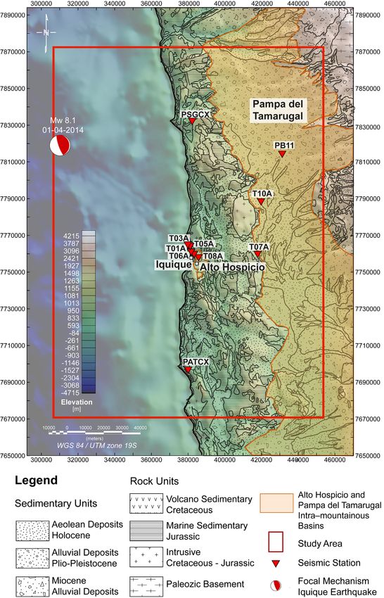
1144       T. Garcı́a-Pérez et al.

amplifications in seismic waves whose wavelengths are comparable           least 13 000 houses and buildings were damaged or destroyed, which
to the width of mountains and the thickness of basins, and also ob-        were mostly located close to the coastal cliff and soft soils areas,
served strong frequency dependency in the degree of amplification.         and thus the damage was attributed to site effects due the region’s
Early analytical studies focused on the incidence of plane waves on        geomorphological features (Hayes et al. 2014; Becerra et al. 2015,
simple layered features, such as semicircular, triangle or rectangular     2016). More generally, given that northern Chile is prone to large
valleys and hills, or simple layered step structures. These studies        earthquakes, understanding the effect of its prominent topographic
found that topographic and geological features can have significant        features and basins on seismic waveforms is the key to interpreting
frequency-dependent effects on seismic waves, ranging from am-             spatial variation of seismic shaking in the region.
plification to de-amplification at given sites (Bouchon 1973; Geli            In this study, we investigate the potential causes of these site
et al. 1988; Faccioli 1991; Sánchez-Sesma et al. 1993; Pedersen           effects by simulating seismic wave propagation in Northern Chile
et al. 1994; Ashford et al. 1997). However, the analytical calcula-        using the spectral element method and, for the first time, the effects

                                                                                                                                                         Downloaded from https://academic.oup.com/gji/article/227/2/1143/6316783 by University College London user on 10 August 2021
tions performed in these studies typically do not reproduce the full       of topography and sedimentary basins on waveforms recorded in
complexity of real data. This led researchers to turn their attention to   Northern Chile are study by the comparison of the simulated wave-
the implementation of advanced numerical modelling techniques,             forms with observations. In order to reduce potential source effects
which have been made possible thanks to advances in computa-               we use two small-moderate magnitude events with magnitudes Mw
tional power (e.g. Bouchon et al. 1996; Komatitsch & Vilotte 1998;         4.5 and 5.4 that occurred as part of the 2014 Iquique earthquake
Paolucci 2002; Álvarez-Rubio et al. 2004; Paolucci & Morstabilini         sequence. This allows us to discuss the likely causes of observed
2006; Lee et al. 2009; Miksat et al. 2010; Fan et al. 2014; Restrepo       amplifications in the region during the 2014 Iquique earthquake, as
et al. 2016). In particular, in the last 20 yr, the spectral element       well as general implications of our results.
method (SEM) has been widely and successfully implemented to
simulate seismic wave propagation in 3-D earth models. The SEM
is a highly accurate technique which allows to account for com-
                                                                           2 GEOLOGICAL FRAMEWORK
plex topographic surfaces, internal discontinuities and sedimentary
basin features (e.g. Komatitsch & Tromp 1999; Komatitsch et al.            As shown in Fig. 1, the main geomorphological features of the
2004, 2010; Lee et al. 2009). However, despite several studies inves-      emerged forearc from 18◦ S to 25◦ S in the study region are, from
tigating the effects of topography and complex geology on seismic          west to east, the coastal plains, the coastal cliff, the coastal cordillera
waves, the poor knowledge of the geometry and mechanical prop-             and the central depression. The coastal plains are a series of narrow
erties of subsoil materials and a lack of validations with real data       (less than 3 km wide) marine abrasion surfaces that are limited to
still limit the understanding of the site effects.                         the east by the 0.5–2-km high coastal cliff (Paskoff 1978; Marquardt
   In recent decades, the instrumental seismic coverage of North-          et al. 2004, 2008; Tolorza et al. 2009; Quezada et al. 2010). Iquique
ern Chile has substantially improved, with an expansion of both            is located in a 3-km wide coastal plain, where stratified rocks are
permanent and temporary seismic networks, including broad-band             covered by thin layers of marine, colluvial and aeolian deposits. The
seismic stations as well as accelerometers (Barrientos 2018). There-       coastal cordillera is made up of Jurassic–Cretaceous volcanic arc
fore, high-quality seismic data are available for the 2014 April 1 Mw      rocks with an average width of about 30 km and a height of between
8.1 Iquique earthquake in Northern Chile, as well as for its fore-         1000 and 2000 m a.s.l. (González et al. 2003; Veiga et al. 2004;
shocks and aftershocks, which provides an excellent opportunity to         Cembrano et al. 2005; Allmendinger & González 2010; Quezada
investigate the causes of the site effects, and notably the interaction    et al. 2010). Several intramountainous basins produced by crustal
between topography, soil properties and seismic waves.                     faulting and filled by sedimentary deposits are located within the
   The 2014 April 1 Mw 8.1 Iquique earthquake was a megathrust             coastal cordillera. In the following paragraphs we describe the most
event produced by subduction of the Nazca plate beneath South              relevant basins for the purpose of the present study, Alto Hospi-
American plate, and its epicentre was located in the widely known          cio and Pampa del Tamarugal. Alto Hospicio is an NS-elongated
Northern Chile seismic gap (Fig. 1). The Northern Chile seismic            basin, which has an average length of ∼8 km, an average width
gap is located in the area between 19◦ S and 23◦ S, within a wider area    of ∼2 km, and is located at an average height of ∼500 m a.s.l.
where the last two major earthquakes occurred in 1868 (approxi-            This basin has a sharp near-vertical boundary next to the coast cliff
mately between 16◦ and 19◦ ) and 1877 (approximately between 19◦           associated with normal faulting processes and has maximum depth
and 22◦ ), both of which had magnitudes of Mw 8.8 (Comte & Pardo           of ∼200–350 m (Marquardt et al. 2008; Garcı́a-Pérez et al. 2018).
1991). Nevertheless the large magnitude of the 2014 Iquique earth-         This basin is one of the few intra-mountain basins that intersects
quake, the potential for a large event in this region still remains,       the coastal cliff, and contains Alto Hospicio city, with a population
given that over 70 per cent of the length of the Northern Chile seis-      of ∼100 000. On the other hand, the Pampa del Tamarugal basin
mic gap has not been released, as shown in Fig. 1 (Bürgmann 2014;         is located in the central depression at a distance of approximately
Hayes et al. 2014; Lay et al. 2014; Ruiz et al. 2014). Additionally,       25 km from the coastline. This basin, located in the central depres-
the Northern Chile region presents notable geomorphological fea-           sion, covers a surface of approximately 300×75 km2 . Similar to
tures in the emerged forearc due to the combined effect of a hyper-        the Alto Hospicio basin, its western boundary is quite sharp, being
arid climate and plate convergence. These features include several         associated with a half-graben produced by normal faults during the
intra-mountainous basins deposited in the coastal cordillera, and a        Mesozoic that reactivate as reverse faults during contraction defor-
steeply sloping coastal cliff with an average height of 1000 me-           mation in the Cenozoic (Galli Olivier & Dingman 1962; Muñoz &
ters (Fig. 1) whose origin is not entirely understood (Paskoff 1978;       Charrier 1996; Mpodozis & Ramos 2008; Bascuñán et al. 2016).
Marquardt et al. 2004; Tolorza et al. 2009; Martinod et al. 2016).         The basin’s northern part is filled by approximately 1000 m of con-
The Iquique earthquake produced peak shaking intensities of VI             tinental deposits and pyroclastic flows, with the towns of Huara and
to VIII on land and ground accelerations of 73.45 per cent (Cilia          Pozo Almonte being located in its western border (Nester & Jor-
et al. 2017; Hayes et al. 2017), in addition a ∼2 m maximum high           dan 2012; Fuentes et al. 2017). The electromagnetic transient TEM
tsunami hit coastal towns from southern Peru to northern Chile. At         geophysical study carried out in the northern part of the Pampa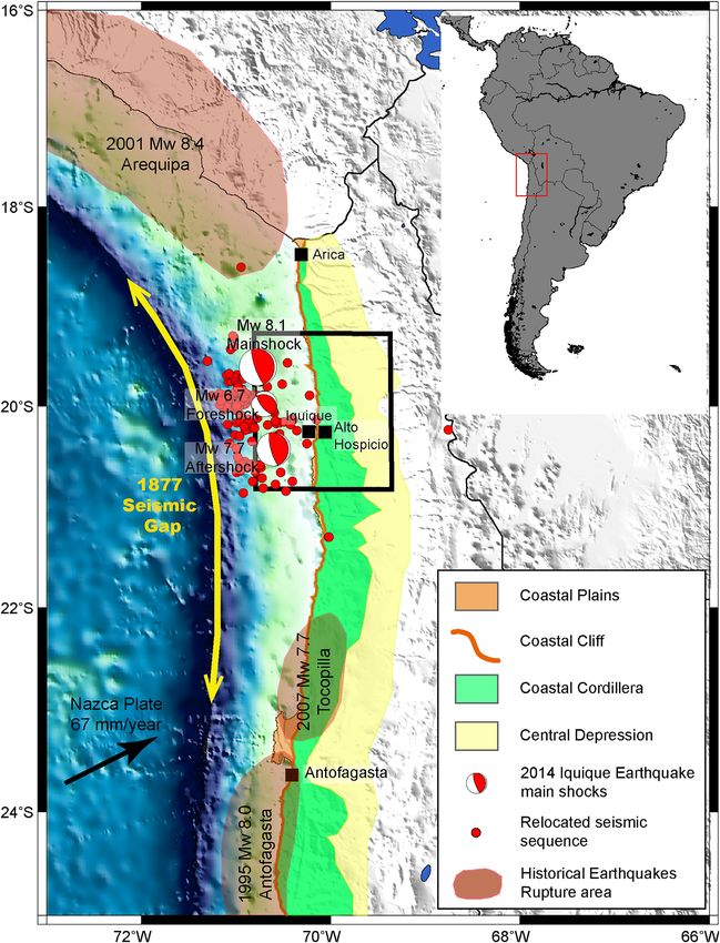
Effects of topography and basins on seismic wave amplification                     1145

                                                                                                                                                               Downloaded from https://academic.oup.com/gji/article/227/2/1143/6316783 by University College London user on 10 August 2021

Figure 1. Topographic map of Northern Chile showing the Iquique earthquake sequence and the main geomorphological units of the emerged forearc. The
red beach balls represent the focal mechanisms of the foreshock, main shock and the main aftershock events, as obtained from the Global CMT catalogue
(Dziewonski et al. 1981 ). The red dots are the relocated seismicity from March to July 2014 as obtained from León-Rı́os et al. (2016). The black rectangle
shows the study area. Dark red shaded polygons represent rupture areas of historical earthquakes. Other elements are described in the inlet legend.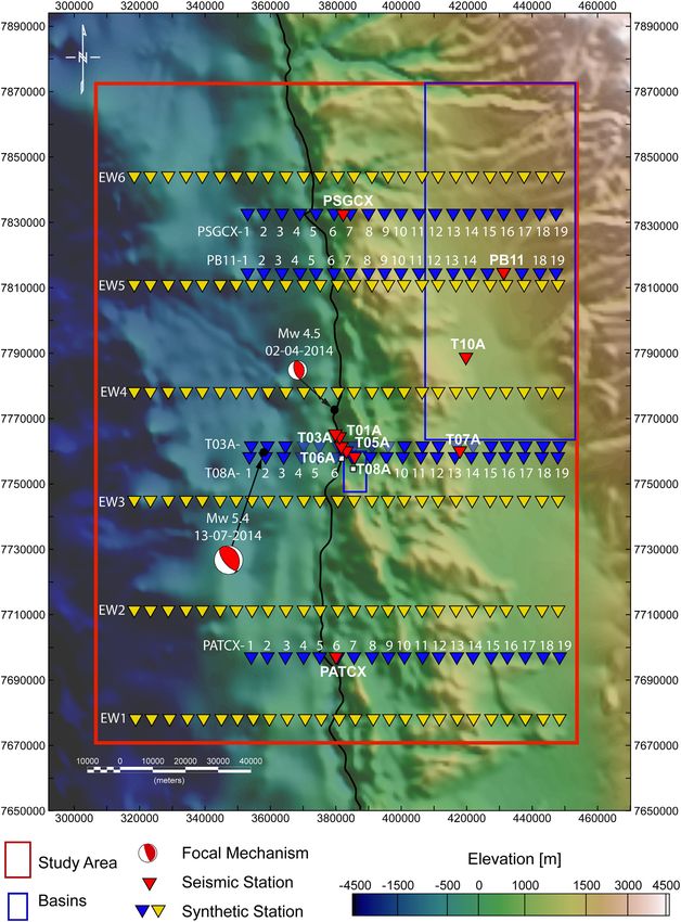
1146       T. Garcı́a-Pérez et al.

del Tamarugal basin agrees with the stratigraphic studies, finding           Fig. 3 shows the processed waveforms for stations T05A, T06A,
basin thickness between 1000 and 1160 m (Viguier et al. 2018).            T03A, T08A and T07A. Stations T03A, T05A and T06 are located
On the other hand, the southern part of the Pampa del Tamarugal           in Iquique in the coastal plain, station T08A is located in Alto
basin is shallower (∼300 m), it is geologically more complex than         Hospicio, which is located within the coastal cordillera approxi-
its northern counterpart (Fig. 2), and its internal structure is poorly   mately 500 m from the coastal cliff, and station T07A is located
constrained, lacking geophysical information in a wide area. Hence,       in the Pampa del Tamarugal Basin at the boundary zone between
in this study we focus on the simpler and better constrained northern     the coastal Cordillera and the central depression (Fig. 2, Table 1).
part of the Tamarugal basin.                                              In the waveforms, clear amplification is visible for stations T03A,
    The geological map in Fig. 2 shows the main geological units in       T08A and T07A, most notably on the horizontal components, since
the study area. In the coastal cordillera some Jurassic and Cretaceous    they show larger amplitudes than stations at shorter epicentral dis-
marine volcano sedimentary rocks are intruded by Cretaceous—              tances. We note that the stations used in Fig. 3 all have about the

                                                                                                                                                     Downloaded from https://academic.oup.com/gji/article/227/2/1143/6316783 by University College London user on 10 August 2021
Jurassic rocks, composed by diorite, granodiorite and granite (Ser-       same source–receiver azimuth, thus, source effects should be about
nageomin 2003; Marquardt et al. 2008; Vásquez & Sepúlveda 2013;         the same for all stations. Given that these three stations are located
López et al. 2017). Above the Jurassic and Cretaceous rocks, Ceno-       either in the vicinity of the coastal cliff or in a sedimentary unit; it
zoic sediments are deposited in the coastal plains, the intramoun-        indicates that the ground motion amplification observed during the
tainous basins within the coastal cordillera, and in the Pampa del        Iquique earthquake may be related to soil type or to the coastal cliff.
Tamarugal basin, in the central depression. Fig. 2 also shows the
locations of the seismic stations used in this study (coordinates are
given in Table 1), which are located over different soil units. As        4 S E I S M I C WAV E F O R M M O D E L L I N G
shown in the Fig. 2, stations PSGCX and PATCX are located in the
                                                                          To understand the effects of the topography and sedimentary in-
coastal cordillera above volcanic rocks; however the station PATCX
                                                                          tramountainous basins on the amplification of the seismic waves,
is located closer to the coastal cliff. Stations T01A, T03A, T05A and
                                                                          we perform simulations of seismic wave propagation in the study
T06A are located in the coastal plain. The stations T01A and T03A
                                                                          region using the Cartesian version of SPECFEM3D, a software
are located above aeolian deposits and stations T05A and T06A are
                                                                          package that uses the spectral element method (SEM) to solve the
located above Jurassic—Cretaceous sedimentary rocks. The station
                                                                          3-D wave equation at local or regional scales (Komatitsch & Vilotte
T08A is located in the Alto Hospicio basin in the coastal cordillera
                                                                          1998; Komatitsch & Tromp 1999; Komatitsch et al. 2010). The SEM
at approximately 500 m a.s.l. On the other hand, the stations T07A
                                                                          is a highly accurate numerical method that uses a mesh of hexahe-
and T10A are located in the eastern part of the coastal cordillera,
                                                                          dral finite elements on which the wavefield is represented in terms
at the limit with the central depression, on alluvial sediments of the
                                                                          of high-degree Lagrange polynomials on Gauss–Lobatto–Legendre
Pampa del Tamarugal basin. Finally, the station PB11 is located in
                                                                          interpolation points. This method and the SPECFEM3D software
the northern part of the Pampa del Tamarugal basin (Pinto Morales
                                                                          have been widely employed to model seismic wave propagation us-
et al. 2016).
                                                                          ing local, regional and global velocity models (e.g. Magnoni et al.
                                                                          2014; Molinari et al. 2015; Parisi et al. 2018); as they combine the
                                                                          flexibility of the finite-element method with the accuracy of pseu-
3 S E I S M I C D ATA : E V I D E N C E F O R S I T E                     dospectral techniques. The flexibility of the mesh allows the im-
EFFECTS                                                                   plementation of complex geometries, topography, bathymetry and
                                                                          basement surfaces with minimal numerical dispersion, and with the
As explained previously, in recent decades, a large number of seis-
                                                                          advantage of traction-free boundary conditions (Faccioli 1991; Ko-
mic stations have been deployed in Northern Chile. The IPOC seis-
                                                                          matitsch & Vilotte 1998; Komatitsch & Tromp 1999; Komatitsch
mic network (see some examples of seismic stations in Fig. 2) is part
                                                                          et al. 2004, 2010; Lee et al. 2009).
of the Integrated Plate Boundary Observatory of Chile, a European–
Chilean seismic network dedicated to the study of earthquakes and
deformation in the continental margin. It is operated by the GFZ
                                                                          4.1 Model implementation
German Research Centre for Geosciences, the Institut de Physique
du Globe de Paris (IPGP), the Chilean Seismological Center (CSN),         In this study, we use a mesh with a width of 145 km, a length of
the Universidad de Chile (UdC) and the Universidad Católica del          200 km and a depth of 60 km, ranging from 19.25◦ S to 21.05◦ S and
Norte (UCNA; Geosciences & CNRS-INSU 2006). The National                  from 69.45◦ W to 70.85◦ W. The number of elements on each side of
Seismological Network (RSN in Spanish) comprises a set of over            the mesh is 320 in the east direction, 320 in the north direction and
95 multiparameter stations located in the Chilean territory, which        120 in the depth direction, obtaining elements with lengths between
includes broad-band seismometers, accelerometers and GPS sen-             453 and 679 m, making a total of 12 288 000 elements. This mesh
sors. Table 1 shows the details of the seismic stations in the study      configuration is chosen so that the source–receiver region consid-
area used in this study and Fig. 2 shows their locations, including       ered is well covered enabling the accurate calculation of synthetic
stations from both the IPOC and RSN networks.                             waveforms with frequencies up to 3.5 Hz, while keeping a reason-
   In order to examine the signature of site effects in the seismic       able computational cost of the simulations. In order to validate the
data, in this section we analyse three-component waveforms gener-         accuracy of our simulations, we have performed simulations with a
ated by the 2014 Iquique earthquake recorded by the RSN seismic           finer mesh with 640 elements in the east direction, 640 elements in
network. We deconvolve the instrument’s response from the wave-           the north direction and 120 elements in the depth direction, with el-
forms and remove the mean and trend. The horizontal-component             ement lengths between 226 and 522 m, making a total of 49 152 000
waveforms are rotated into radial (R) and transverse (T) direc-           elements. Supporting Information Fig. S1 compares waveforms ob-
tions. The data are filtered using a Butterworth bandpass filter of       tained with these two different meshes filtered in frequency ranges
order 2 with four poles in various frequency bands from 0.01 to           between 0.1 and 2.0 Hz. These graphs show good agreement be-
20 Hz.                                                                    tween the two sets of synthetics for some representative stations.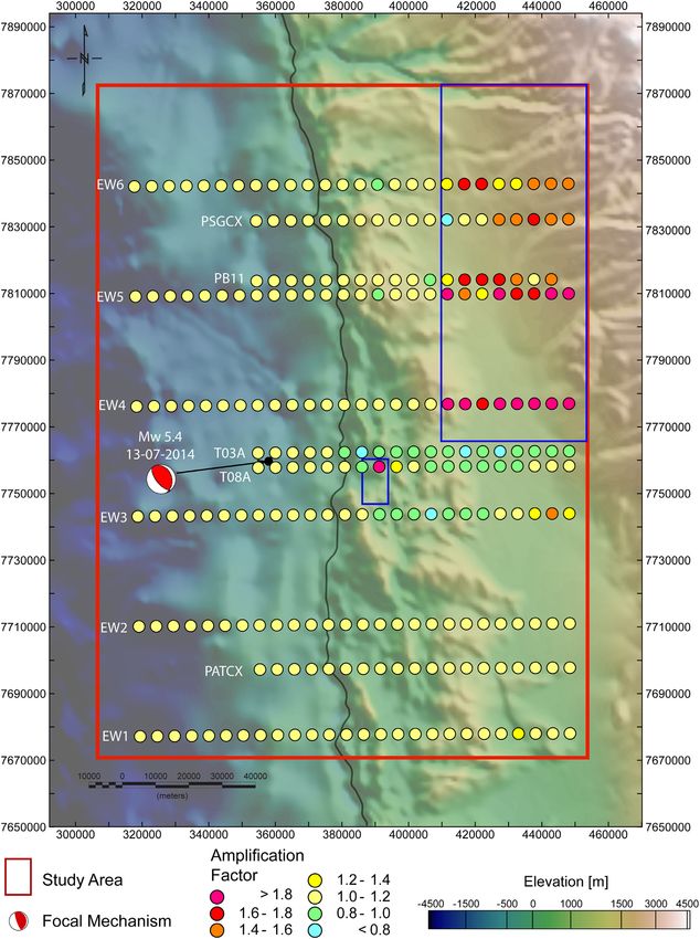
Effects of topography and basins on seismic wave amplification                       1147

                                                                                                                                                                 Downloaded from https://academic.oup.com/gji/article/227/2/1143/6316783 by University College London user on 10 August 2021

Figure 2. Geological map of the study area (red rectangle) above the SRTM topographic map in WGS84 datum 19S (Becker et al. 2009). The inverted red
triangles show the locations of seismic broad-band stations from the IPOC and RSN seismic networks used in this study (see the main text for further details).
The red beach ball represents the focal mechanism of the 2014 April 1 Iquique earthquake. The annotations ‘Pampa del Tamarugal’ and ‘Alto Hospicio’
highlight the locations of these sedimentary basins.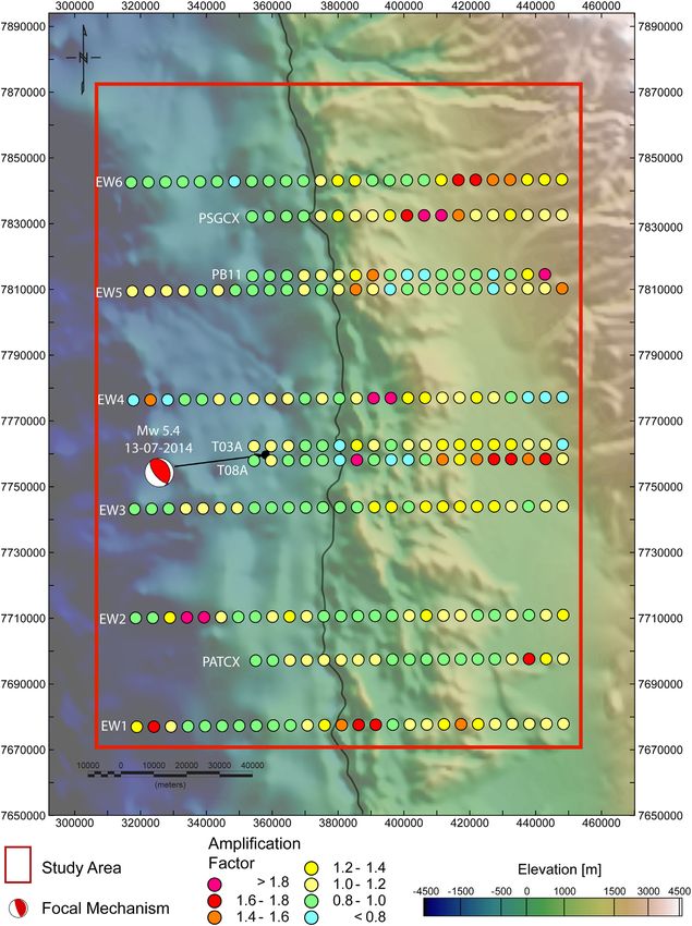
1148 T. Garcı́a-Pérez et al.
These results validate the accuracy of the meshes and justifying the
Sampling rate (s−1 )
use of the coarser mesh, which leads to computationally cheaper
simulations by about a factor of six.
200
200
100
100
200
200
100
200
200
200
We use a 1-D earth model of P- and S-wave speed that was used
by León-Rı́os et al. (2016) to determine the hypocentral locations
of the Iquique earthquake sequence. It is a modification of a model
built by Husen et al. (1999) for the Antofagasta region (300 km
south of Iquique), as presented in Fig. 4. We set the shear attenuation
coefficient to 600 for all depths and use Stacey absorbing conditions
for the four vertical faces and for the bottom face of the grid in order
to simulate a semi-infinite regional medium of elastic elements and
Downloaded from https://academic.oup.com/gji/article/227/2/1143/6316783 by University College London user on 10 August 2021
Kinemetrics Episensor FBA
Kinemetrics Episensor FBA
Kinemetrics Episensor FBA
Kinemetrics Episensor FBA
Kinemetrics Episensor FBA
Kinemetrics Episensor FBA
Kinemetrics Episensor FBA
a free-surface condition at the top. The sampling interval is set at
0.005 s and the maximum resolvable frequency is 3.5 Hz, as roughly
Streckeisen STS2 5 points per wavelength are needed to sample the wave field. The
Streckeisen STS2
Streckeisen STS2
computations were performed on the UK’s national supercomputing
Instrument type
facility ARCHER using parallel programming that distributes the
320 mesh slices over 20 processors for each coordinate axis, using
a total of 400 processors for a total of 12 288 000 elements. Each
simulation had a duration of approximately 5 hr on ARCHER.
To investigate the separate effects of topography and basins on
seismic wave amplification we performed seismic wave propagation
simulations using three different earth models:
Sedimentary Rock
Sedimentary Rock
Alluvial Deposits
Alluvial Deposits
Alluvial Deposits
Alluvial Deposit
Aeolian Deposit
Aeolian Deposit
(i) A flat model (i.e. with neither topography nor basins) using
Volcanic Rock
Volcanic Rock
the 1-D velocity model described above;
Soil type
(ii) A model with topography and the 1-D velocity structure.
We implemented the Shuttle Radar Topography Mission (SRTM)
Digital Elevation Model (Becker et al. 2009) for our study region
with a 90 m resolution in the surface of the grid. However, since the
spacing of the mesh (which has element lengths between 453 and
679 m) is coarser than the resolution of the DEM, the topography
was smoothed when building the mesh, yet preserving the important
Pampa del Tamarugal Basin
Pampa del Tamarugal Basin
Pampa del Tamarugal Basin
features, such as the coastal cliff, as shown in Fig. 5(a). Moreover,
Supporting Information Fig. S2 shows some illustrative examples
Geomorphologic unit
Alto Hospicio Basin
of EW profiles, shown in Fig. 6, of the implemented topography
Coastal Cordillera
Coastal Cordillera
compared with that in the DEM;
Coastal Plain
Coastal Plain
Coastal Plain
Coastal Plain
(iii) A basin model whereby two cuboids with different sizes and
Table 1. Details of the seismic stations in Northern Chile used in this study (see Fig. 2).
elastic properties are added to the topographic model. These two
cuboids represent the Alto Hospicio and the northern part of the
Pampa del Tamarugal basins, with density, Vp and Vs values related
to sedimentary geological units (Teldford et al. 1990; Dentith &
Mudge 2014). The geometry of the basins was obtained from the
Elevation (m a.s.l)
previous studies of Garcı́a-Pérez et al. (2018) and Viguier et al.
(2018), both of which constrained the extension and depth of the
1049
1007
1400
970
805
223
536
31
33
11
sedimentary deposits filling the basins using geophysical data. Ta-
ble 2 shows the geometric parameters that were used to simulate the
basins in the mesh, in which the Alto Hospicio (AH) basin is smaller
(8 km in length, 2 km in width and 500 m in depth), being located in
the middle of the mesh next to the coastal cliff, while the northern
Lon (◦ W)
part of the Pampa del Tamarugal (PT) basin is larger, being located
70.120
70.150
70.138
70.122
70.146
69.786
70.094
69.767
69.990
70.150
in the upper right part of the mesh. As explained previously, in this
study we focus on the northern part of the Pampa del Tamarugal
basin, as it is the deepest and better constrained part of the basin.
Fig. 5(b) shows the tridimensional basin model.
Lat (◦ S)
19.600
20.273
20.230
20.210
20.214
20.256
20.270
19.995
19.760
20.820
4.2 Earthquakes studied
For each model used, we consider two small-to-moderate magnitude
earthquakes using the source parameters and hypocentral locations
Station ID
obtained from the analysis of León-Rı́os et al. (2016; Table 3).
PSGCX
PATCX
T01A
T03A
T05A
T06A
T07A
T08A
T10A
PB11
These earthquakes occurred as part of the aftershock sequence of
the Iquique earthquake and their hypocentres were located at 34 and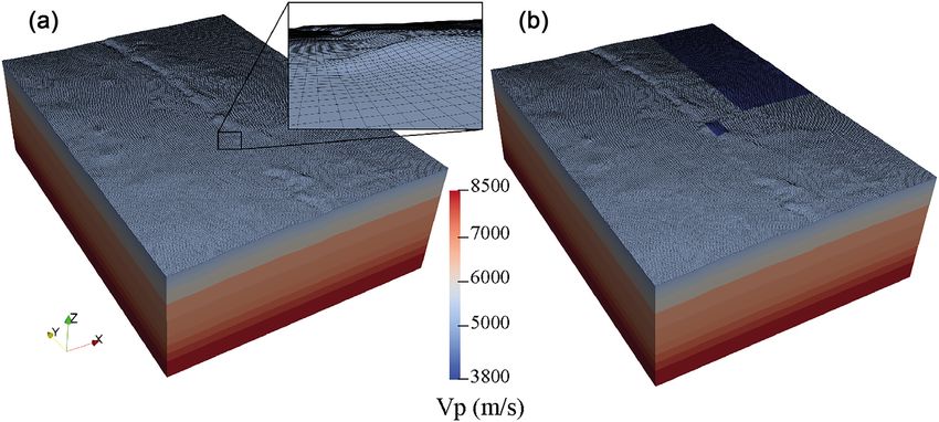
Effects of topography and basins on seismic wave amplification                       1149

                                                                                                                                                                 Downloaded from https://academic.oup.com/gji/article/227/2/1143/6316783 by University College London user on 10 August 2021
Figure 3. Examples of local acceleration waveforms for the 2014 April 1 Mw 8.1 Iquique earthquake measured by five three-component seismic stations
located at various epicentral distances, showing evidence for site effects (see Fig. 2 for the location of the stations). The waveforms were filtered using a
Butterworth bandpass filter of order 2 with four poles in various frequency bands from 0.1 to 20 Hz. The vertical (Z, left), radial (R, middle) and transverse
(T, right) components for the five stations are shown using the same horizontal and vertical scales. The red circles represent the maximum peak value for each
trace, with the value also annotated in red.

49 km depth, close to the emerged continental forearc, as shown in                both models filtered in four different frequency ranges between 0.1
Fig. 6. The events were earthquakes with focal mechanisms very                    and 2.0 Hz (0.1–0.2 Hz, 0.2–0.5 Hz, 0.5–1.0 Hz and 1.0–2.0 Hz).
similar to that of the main shock but with smaller magnitudes of                  Fig. 7 shows the waveforms filtered between 0.5 and 1.0 Hz for
Mw 5.4 and 4.5, respectively. We choose this magnitude range to                   some stations along the profile PSGCX (see location in Fig. 6), in
avoid the extended source complexity effects which are associated                 which three main effects related to topography can be seen. First,
with larger earthquakes while ensuring a good signal-to-noise ratio               as expected, there is a small time-shift between the two sets of
of the observed waveforms.                                                        waveforms due to the difference in altitude between the flat and
   As the number of stations used in the SEM simulations does                     the topographic model. Second, differences in amplitude can be ob-
not increase their computational cost, we compute synthetic seis-                 served between the three-component waveforms at some stations
mograms both for the locations of real stations in the region (red                (e.g. PSGX6 and PSGCX7) close to important topographic features
triangles in Fig. 6) and for a number of hypothetical stations (blue              such as the coastal cliff. Finally, the simulations that include topog-
and yellow triangles in Fig. 6). The synthetic stations in blue repre-            raphy show reflected waves produced in the coastal cliff, which ap-
sent stations which are situated at the same latitude as a real station           pear as a secondary arrival in the vertical and radial components for
and are positioned at various longitudes to allow a west–east profile             some stations (see stations PSGCX8, PSGCX9, PSGCX10 marked
to be constructed, whereas the synthetic stations in yellow are used              with red arrow in Fig. 7) and have the same or slightly larger ampli-
to construct completely synthetic profiles in order to increase the               tudes than the main waveforms (see stations PSGCX12, PSGCX14,
spatial coverage across the mesh.                                                 PSGCX16 and PSGCX18 marked with red arrow in Fig. 7).
                                                                                     To estimate the ground motion amplification generated by the
                                                                                  topography, we calculate the ratio between the total energy obtained
5 M O D E L L I N G R E S U LT S                                                  from the velocity seismograms, filtered between 0.1 and 3.5 Hz, for
                                                                                  the topographic and flat models and for each station. The total
5.1 Topographic model simulation                                                  energy is the integral of the square of the ground velocity of the
To investigate the effects of topography on seismic wave propaga-                 three components for each type of seismogram. Then we compute
tion in the study region, we show the simulations performed for the               the ratio of the total energies for the topographic and flat models.
2014 July 13 Mw 5.4 earthquake (depth ∼34 km; Table 3) using                      The energy amplification-ratio between the topographic model and
the flat model and the topographic model combined with the 1-D                    the flat model in every simulated station is shown as coloured circles
earth structure described in Section 4.1. Fig. 7 and Supporting Infor-            from light-blue to pink, as shown in Fig. 8. We note that the approach
mation Figs S3–S6 compare the synthetic waveforms obtained for                    that we use to estimate amplification is different than others in the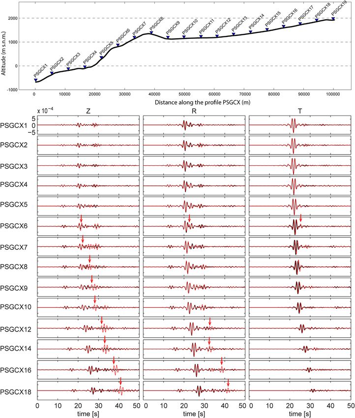
1150       T. Garcı́a-Pérez et al.

                                                                            observed in stations near the coastal line and in the coastal cordillera,
                                                                            which is spatially related to the coastal plains and valleys into the
                                                                            coastal cordillera. For low frequency ranges, 0.1–0.2 Hz and 0.2–
                                                                            0.5 Hz, an area of deamplification is observed near the coastal
                                                                            cliff. However, this deamplification disappears at higher frequen-
                                                                            cies, for which a large area of deamplification develops inland near
                                                                            valleys.

                                                                                                                                                        Downloaded from https://academic.oup.com/gji/article/227/2/1143/6316783 by University College London user on 10 August 2021
                                                                            5.2 Basin model simulation
                                                                            In order to investigate the effect of the region’s basins on the wave-
                                                                            forms, in this section we show the results of the simulations per-
                                                                            formed for the 2014 July 13 Mw 5.4 earthquake using the 1-D
                                                                            velocity model with topography and the 1-D velocity model with
                                                                            topography and basins, in which sedimentary basins in the region
                                                                            are simulated as described in Section 4.1 and represented in Fig. 6
                                                                            (blue rectangles). Fig. 10 compares synthetic waveforms for some
                                                                            stations, filtered between 0.5 and 1.0 Hz, obtained from both mod-
                                                                            els for the stations along the T08A profile, which crosses the Alto
                                                                            Hospicio basin from west to east. Supporting Information Figs S7–
                                                                            S10 present the synthetic waveforms for all the stations along the
                                                                            T08A profile filtered between 0.1–0.2 Hz, 0.2–0.5 Hz, 0.5–1.0 Hz
                                                                            and 1.0–2.0 Hz. From a comparison of the two types of synthetic
                                                                            waveforms in Fig. 10 it can be seen that the differences between
                                                                            them are not significant until the seismic wavefield reaches the sta-
                                                                            tions T08A7 and T08A8, which are located in the area surrounding
Figure 4. The 1-D model of Vp , Vs and density (Husen et al. 1999; León-   the Alto Hospicio basin. These two stations show amplification of
Rı́os et al. 2016) used in this study.                                      the seismic wavefield in the vertical and transverse components.
                                                                            However, the amplitude of the radial component is smaller for the
                                                                            model with topography and basins (blue trace in Fig. 10) than for the
literature (e.g. Boore 1972; Olsen 2000; Poursartip et al. 2017),           topography-only model (red trace in Fig. 10). On the other hand, the
which are often based on ratios of peak ground velocity. In this            seismic stations further to the east (from T08A9 to T08A19) show
study occasionally the peak velocity of the secondary waves is larger       slight differences in amplitude between the transverse component
than that of the main waveform (e.g. Fig. 7), which is problematic.         waveforms obtained for the two models, which is probably due to
Hence, we prefer to estimate amplification based on energy ratios           the reflection of waves in the Alto Hospicio basin (see from ∼19 s
obtained from three-component seismograms.                                  onward in movie basin en the supplementary material). Support-
   In Fig. 8, a clear spatial relationship can be observed for              ing Information Figs S11–S14 present synthetic waveforms filtered
amplification-ratio > 1 (circles coloured in yellow, orange, red and        between 0.1–0.2 Hz, 0.2–0.5 Hz, 0.5–1.0 Hz and 1.0–2.0 Hz for
pink in Fig. 8) which includes the coastal cordillera, which is limited     the PB11 profile, where the amplification effects of the Pampa del
to the west by the coastal cliff and the coastline (black line). On the     Tamarugal basin are clearly shown, where it is possible to observe
other hand, we observe that topographic deamplification ratio < 1           amplification of the waves and that total duration of the waveforms
(light-blue and green coloured circles in Fig. 8) is mainly spatially       qualitatively increases.
related to the offshore area and valleys located within the coastal            As in the previous section, Fig. 11 shows a map with the total
cordillera (green regions in Fig. 6). For simplicity, in the remainder      energy ratio between the model with topography and basins and
of this paper we shall refer to amplification-ratio > 1 as ampli-           the topography-only model represented in coloured circles. This
fication and to deamplification ratio < 1 as deamplification. The           ratio was computed in the same way as in Section 5.1. Fig. 11
amplification reach values of up to 2.16 (i.e. amplification of 116         shows that there is clear amplification in the stations located within
per cent) and deamplification as low as 0.55 (i.e. de-amplification         basins (blue rectangles), with the amplification ratio reaching up to
of 45 per cent).                                                            2.9 (representing a 190 per cent increase in amplitude), as well as
   In Fig. 9, amplification-ratio maps for frequencies ranges be-           amplification ratios of up to 1.25 (25 per cent increase in amplitude)
tween 0.1–0.2 Hz, 0.2–0.5 Hz, 0.5–1.0 Hz and 1.0–2.0 Hz are                 in stations in the far southeast region of the study area. Additionally,
shown. In these maps, maximum amplification-ratios of 1.35,                 Fig. 11 also shows that there is clear deamplification up to 0.75 (25
1.53, 3.38 and 3.6 are observed for the frequency ranges of 0.1–            per cent decrease in amplitude) in areas surrounding the basins.
0.2 Hz, 0.2–0.5 Hz, 0.5–1.0 Hz and 1.0–2.0 Hz respectively. The             The energy ratio maps for frequency ranges of 0.1–0.2 Hz, 0.2–
results show amplifications produced in the surrounding area of             0.5 Hz, 0.5–1.0 Hz and 1.0–2.0 Hz are presented in Fig. 12 showing
the coastal cliff increase with the frequency, with the lowest val-         that the amplification generally increases with frequency, reaching
ues being observed in the lowest frequency range, that is, 0.1–             a maximum value of 3.9 for stations located in the Pampa del
0.2 Hz, and the largest values of 3.6 being observed in the fre-            Tamarugal basin and a maximum value of 1.8 for the station located
quency ranges of 1.0–2.0 Hz. In the same way, deamplification is            in the Alto Hospicio basin for the frequency range 1.0–2.0 Hz.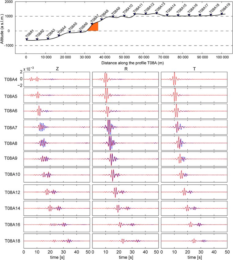
Effects of topography and basins on seismic wave amplification                   1151

                                                                                                                                                           Downloaded from https://academic.oup.com/gji/article/227/2/1143/6316783 by University College London user on 10 August 2021
Figure 5. 3-D view of the mesh used in this study, which is 200 km long, 145 km wide and 60 km deep. The 1-D Vp values which were implemented are also
shown. (a) 1-D velocity model for Vp ranging from 3800 to 8050 m s−1 with topography. (b) 1-D velocity model with topography and basins, with Vp ranging
from 3800 to 8050 m s−1 . Both basins considered are shown in dark blue: the smaller Alto Hospicio basin (8 km long, 2 km wide and 500 m deep) and the
larger Pampa del Tamarugal basin (105 km long, 50 km wide and 1000 m deep).

6 C O M PA R I S O N W I T H R E A L D ATA                                     for the different models show that there are only slight differences
                                                                               between the waveforms obtained for the topography and the topog-
In this section, we compare the different synthetic waveforms ob-
                                                                               raphy and basins models for the stations T03A, T07A, PSGX and
tained in this study with real data for the 2014 April 2 Mw 4.5
                                                                               PATCX, while more significant differences are observed for those
and the 2014 July 13 Mw 5.4 earthquakes. As explained previously,
                                                                               stations located within or around the modelled basins (T08A, T10A
these earthquakes were chosen due to the similarity of their focal
                                                                               and PB11). Overall, good fits (time phase misfit values close to 0 s
mechanisms with the main 2014 April 1 Mw 8.1 Iquique earthquake,
                                                                               and amplitude misfit values close to 1) are obtained between the
but their smaller magnitudes allow us to avoid the extended source
                                                                               real and the synthetic waveforms for stations T07A and PSGCX,
complexity effects in the real data and visualize more precisely site
                                                                               with some time-shifts and differences in amplitude, mostly in the
effects. As the RSN network provides acceleration data, we double-
                                                                               radial and transverse components. Station T10A also shows good
differentiate the IPOC data and all the synthetic seismograms to
                                                                               fit for the 1-D topography model, while the fit gets worse for the
obtain acceleration values for all the stations considered. The real
                                                                               1-D topography and basins model. For stations T03A, T08A, PB11
data and the synthetic seismograms are processed in the same way
                                                                               and PATCX, larger differences are observed between the real data
by removing the trend and the mean and by rotating the horizontal
                                                                               and the synthetic seismograms (phase misfits values above 0.5 s and
components into radial and transverse components. Finally, all the
                                                                               amplitude misfit values less than 0.5, meaning that the amplitude
waveforms are band pass filtered with a four-pole two-pass Butter-
                                                                               of the synthetics are less than half the amplitude of the real data).
worth filter for different frequency ranges between 0.1 and 2.0 Hz.
                                                                               Stations PB11 and T08A are located in the Pampa del Tamarugal
We compare the synthetic and real waveforms by computing the
                                                                               and Alto Hospicio basins, respectively (Fig. 2) and, despite the fact
cross-correlation between the waveforms to obtain the phase mis-
                                                                               that the wave amplitudes obtained using the model with topography
fits and for the amplitude misfits we calculated the square root of the
                                                                               and basins show differences to those obtained using the topographic
ratio between the sum of the square of the amplitudes in the synthet-
                                                                               model, the real data is much more complex with larger amplitudes
ics and the real data. In this way, for the phase misfit values close to
                                                                               than the synthetic waveforms for the basin model. The disagree-
0 and for the amplitude misfit values close to 1 are considered good
                                                                               ment between the real data and the synthetic waveforms obtained
fits.
                                                                               using the basin model is probably due to the simplified geome-
                                                                               try and elastic properties of the basin used in our simulations. On
6.1 Simulation of the 2014 April 2 Mw 4.5 Earthquake                           the other hand, stations T03A and PATCX show larger differences
                                                                               in phase and amplitude between the real data and the synthetics,
The Mw 4.5 earthquake of 2014 April 2 was located at a depth                   probably related to the proximity of these stations with the coastal
of 49 km, with the hypocentre located close to the coastline. To               cliff. When considering different frequency ranges (see Supporting
compare the real data and the computed waveforms, we simulate this             Information Figs S15–S18), the differences between the real and
earthquake using the different models as explained in Section 4.1. In          synthetic waveforms increases as frequency increases, with notable
this section we show the simulations using the 1-D velocity model              good agreements for the frequency range between 0.1–0.2 Hz, but as
with topography and the 1-D velocity model with both topography                frequency increases the observations are more complex and often
and basins.                                                                    having larger amplitudes than the synthetics (see Supporting In-
   The comparison of the synthetic waveforms obtained from these               formation Fig. S23, showing large amplitude misfits for frequency
simulations with the corresponding real data is shown in Fig. 13               ranges between 0.5 and 2 Hz). Hence, the amplification in real data
for the frequency range between 0.2–0.5 Hz (Supporting Informa-                is larger than in the synthetics for the higher frequencies, which
tion Figs S15–S18 show the comparison for the frequency ranges                 is likely due to 3-D small-scale heterogeneity that is not yet con-
0.1–0.2 Hz, 0.2–0.5 Hz, 0.5–1.0 Hz and 1.0–2.0 Hz). The results                strained and not accounted for in the modelling.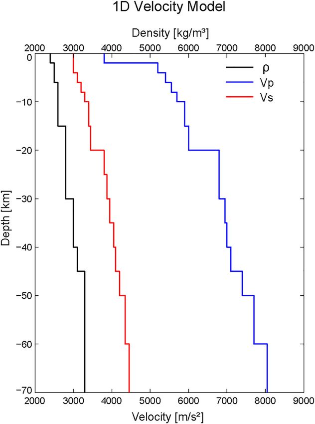
1152        T. Garcı́a-Pérez et al.

                                                                                                                                                                      Downloaded from https://academic.oup.com/gji/article/227/2/1143/6316783 by University College London user on 10 August 2021

Figure 6. SRTM topographic map (Becker et al., 2009) of the study area in WGS84 datum 19S including the focal mechanisms (León-Rios et al. 2016) of
the two aftershock earthquakes considered in this study (red beach balls) and the locations of real seismic stations in the region (red inverted triangles) as well
as hypothetical stations (blue and yellow inverted triangles) aligned along lines of constant latitude. Valleys correspond to green colours while brown colours
correspond to peaks in the Coastal Cordillera.

                               Table 2. Basin model parameters. AH denotes the Alto Hospicio basin and PT denotes the
                               Northern part of the Pampa del Tamarugal basin (see Fig. 5b).
                                            Density (kg                      Vs (m
                               Basin          m−3 )          Vp (m s−1 )     s−1 )     Length (km)     Width (km)     Depth (km)
                               AH              2400             3800         2500           8               2              0.5
                               PT              2400             3800         2500          105             50               1
Effects of topography and basins on seismic wave amplification 1153
Table 3. Source parameters of the earthquakes used in this study.
Date Earthquake ID Location Focal mechanism
Lat (◦ ) Lon (◦ ) Depth (km) Mw Strike (◦ ) Dip (◦ ) Rake (◦ )
2014–04–02 20140402070345 –20.14 –70.15 49 4.5 350 30 95
2014–07–13 20140713205414 –20.25 –70.36 34 5.4 140 55 80
6.2 Simulation of the 2014 July 13 Mw 5.4 earthquake some arrows). These reflected waves increase the amplitude of the
incident waves at the top of the topographic feature and propagate
Downloaded from https://academic.oup.com/gji/article/227/2/1143/6316783 by University College London user on 10 August 2021
For the 2014 July 13 Mw 5.4 earthquake, as in the previous section,
to the surrounding areas. As the distance between the topographic
we perform simulations using the models explained in Section 4.1.
feature that produced the reflected wave and the observation point
In this section we show the simulation using the 1-D velocity model
increases, the time separation between the incident and the reflected
with topography and the 1-D velocity model with both topography
wave also increases, which in turn increases the duration of ground
and basins.
motion. Our results show that the amplitude of the reflected waves
Fig. 14 shows the comparison of the synthetic waveforms ob-
can be larger than the incident waves in some locations (see e.g.
tained from these simulations with the corresponding real data for
stations PSGCX-12, PSGCX-14, PSGCX-16 in Fig. 7 and Support-
the frequency range between 0.2–0.5 Hz and overall there is a good
ing Information Fig. S4), having important implications for seismic
fit between the simulated and real data for stations T01A, T08A and
hazard in locations close to topographic features (Sánchez-Sesma
T07A (phase misfit values close to 0 seconds and amplitude ratio
& Campillo 1993).
misfit values close to 1 for almost all components), whereas stations
Previous studies, using displacement, acceleration and acceler-
PATCX, PSGCX and PB11 present poorer fits, with phase misfit val-
ation response spectra, reported topographic seismic amplification
ues above 1 second in some components and amplitude misfits less
factors between 2 and 75 per cent, and found that amplification
than 0.5 or higher to 1.5 for some components. Time-shifts and
generally occurs at the slopes and at the top of topographic fea-
some differences in amplitude are observed between the simulated
tures whereas deamplification occurs at the bottom of slopes (e.g.
waveforms using the topographic model and the basin model for
Boore 1972; Bouchon et al. 1996; Paolucci 2002; Buech et al.
stations T01A and T08A, which can be attributed to the simulated
2010). In this study, we found that, for the frequency range 0.1–
Alto Hospicio basin; and for station PB11, related to the simulated
3.5 Hz, the energy amplification factor between the flat and topo-
Pampa del Tamarugal basin. Similar to the Mw 4.5, 2014 April 2
graphic models reaches up to 2.2 (amplification of 120 per cent)
event, the differences between the real and simulated waveforms
and that areas of amplification (i.e. amplification factor > 1) are
increase with increasing frequency range (Supporting Information
strongly spatially related with the top of topographic features such
Figs S19–S22 and cross-correlation and amplitude ratio misfits in
as the coastal cordillera (Figs 7 and 8). On the other hand, ar-
Supporting Information Fig. S23) showing that synthetic wave-
eas of deamplification are observed in valleys formed between
forms perform less well in reproducing the complexity of real data
hills, where amplification factors can reach values of 0.6 (i.e. 40
at frequencies above 0.5 Hz.
per cent deamplification), which agrees with the aforementioned
Moreover, the fit between the real and simulated waveforms dete-
studies.
riorates with increasing epicentral distance (e.g. PSGCX and PB11;
The analysis of different frequency ranges shows that, for stations
see Supporting Information Fig. S23 showing the waveform phase
located east of the coastline, the degree of amplification increases as
and amplitude misfits as a function of epicentral distances, where it
the frequency increases, and the amplification is spatially related to
is possible to see that the misfits deteriorate with epicentral distance
the coastal cliff and the coastal cordillera. The results also suggest
and with increasing frequency). This shows that the 1-D velocity
that areas of amplification and deamplification are related to the
model used in this study is only appropriate for short epicentral
size of the topographic features, where large topography features
distances. For larger distances, a more complex velocity model is
such as the coastal cliff (500–1000 m high) or the coastal cordillera
needed, as the shallow depth of the hypocentre and the large dis-
(50 000 m width) produce major effects in the 0.1–0.5 Hz frequency
tance from the coastal line of the 2014 July 13 earthquake leads
range, while smaller features such as hills and valleys in the coastal
to shallower source–receiver paths, which are strongly affected by
cordillera (with ∼50–100 m heights and ∼1000–3500 m width),
small-scale crustal heterogeneity. Moreover, we also note that e.g.
produce effects in the 1.0–2.0 Hz frequency range (see Fig. 9).
for station PSGCX, the ray paths for the 2014 July 13 earthquake
The dependency between seismic amplification due to topography
are mostly oceanic while those for the 2014 April 2 event are mostly
and frequency has been investigated in several studies. For exam-
continental, which may also explain the differences in data fit for
ple, in the Little Red Hill experimental study presented by Buech
the two events.
et al. (2010), their frequency-domain analysis shows a maximum
amplification at about 5 Hz, a frequency close to the first resonant
7 DISCUSSION harmonic frequency equal to the half-width or the height of the
edifice. In the same way, the effects observed for a 3-D ellipsoid
7.1 Topography effects hill studied by a semi-analytical semi-numerical method show that
amplification occurs at and near the top of the hill over a broad range
Our study shows that topography modifies the seismic ground mo- of frequencies, and the maximum amplification value depends on
tion response in Northern Chile by changing the amplitude and the geometry of the features (Bouchon et al. 1996). In general,
duration of waveforms due to reflections generated by the topo- the frequency of maximum amplification corresponds to the wave-
graphic features (see time 12–15 s Supporting Information Movie length comparable with the mountain width (Geli et al. 1988 and
S1 and Fig. 7, where some examples of reflections are highlighted by1154 T. Garcı́a-Pérez et al.
Downloaded from https://academic.oup.com/gji/article/227/2/1143/6316783 by University College London user on 10 August 2021
Figure 7. Top: Topography of the PSGCX profile (Fig. 6). Bottom: Comparison of synthetic seismograms computed using the 1-D flat model (black line) and
the 1-D model with topography (red line) for the 2014 July 13 earthquake. The synthetic seismograms are all bandpass filtered between 0.5 and 1.0 Hz. The
processed waveforms for the vertical (left), radial (centre) and transverse (right) components are shown for 14 of the 19 stations along the PSGCX profile
(Fig. 6). Red arrows indicate secondary waves produced by topography.
references therein), which is consistent with the results obtained in the SEM. They used a LiDAR digital terrain model (DTM) of
this study. the Yangminshan region in Taiwan to implement a high-quality
Our results also agree with the findings of Lee et al. (2009), topographic model using a 4 × 4×10 km3 mesh with resolu-
who investigated seismic amplification due to topography using tion of 2 m. They obtained PGA amplification of around 50Effects of topography and basins on seismic wave amplification 1155
Downloaded from https://academic.oup.com/gji/article/227/2/1143/6316783 by University College London user on 10 August 2021
Figure 8. Map showing the energy amplification ratio for the frequency range between 0.1 and 3.5 Hz in the velocity waveforms between synthetic seismograms
obtained using the flat model and the model with topography. The map shows coloured circles for each station location, in which the colours represent the
calculated amplification factor with values between < 0.8 and > 1.8. Values above 1 represent relative amplification between the flat and topography models,
while values below 1 represent relative deamplification. The beach ball represents the Mw 5.4 2014 July 13 earthquake. The grey-shaded elevation map shows
the geomorphological features related to the coastal cliff and the coastal cordillera to the east of the coastal line (black line).
per cent due to variations in topography in mountainous areas, 7.2 Basin effects
which agrees with our results, despite the fact that we used a
As expected, we found that basins have a significant impact on the
lower-resolution mesh (∼450–680 m) in a much larger domain
ground motion response: they increase the amplitude and duration
(145 × 200 × 60 km3 ).1156 T. Garcı́a-Pérez et al.
Downloaded from https://academic.oup.com/gji/article/227/2/1143/6316783 by University College London user on 10 August 2021
Figure 9. Amplification ratio maps between flat and topography models for frequency ranges between 0.1–0.2 Hz, 0.2–0.5 Hz, 0.5–1.0 Hz and 1.0–2.0 Hz.
The maps show coloured circles for each station location, in which the colours represent the calculated amplification factor. Values above 1 represent relative
amplification between the flat and topography models, while values below 1 represent relative deamplification. The beach ball represents the Mw 5.4 2014
July 13 earthquake. The grey-shaded elevation map shows the geomorphological features related to the coastal cliff and the coastal cordillera to the east of the
coastal line (black line).Effects of topography and basins on seismic wave amplification 1157
Downloaded from https://academic.oup.com/gji/article/227/2/1143/6316783 by University College London user on 10 August 2021
Figure 10. Top: Topography of the T08A profile (Fig. 6), orange polygon represents the modelled Alto Hospicio basin. Bottom: Comparison of synthetic
seismograms computed using the 1-D velocity model with topography (red line) and the 1-D velocity model with topography and basins (blue line) for the
2014 July 13 earthquake. The synthetic seismograms are all bandpass filtered between 0.5 and 1.0 Hz. The processed waveforms for the vertical (left), radial
(centre) and transverse (right) components are shown for 11 of the 19 stations of the T08A profile (Fig. 6).
of the incident seismic waves and produce reflections on their edges (Fig. 11), amplification occurs in the interior of the basins, reach-
that propagate both within the basin and in the surrounding areas ing amplification ratios of up to 2.9 in the Pampa del Tamarugal
(e.g. Celebi 1987; Frankel et al. 2002; Semblat et al. 2005; Paolucci basin and 1.8 in the Alto Hospicio basin. The analysis of the am-
& Morstabilini 2006). plification in different frequency ranges (Fig. 12) indicates that the
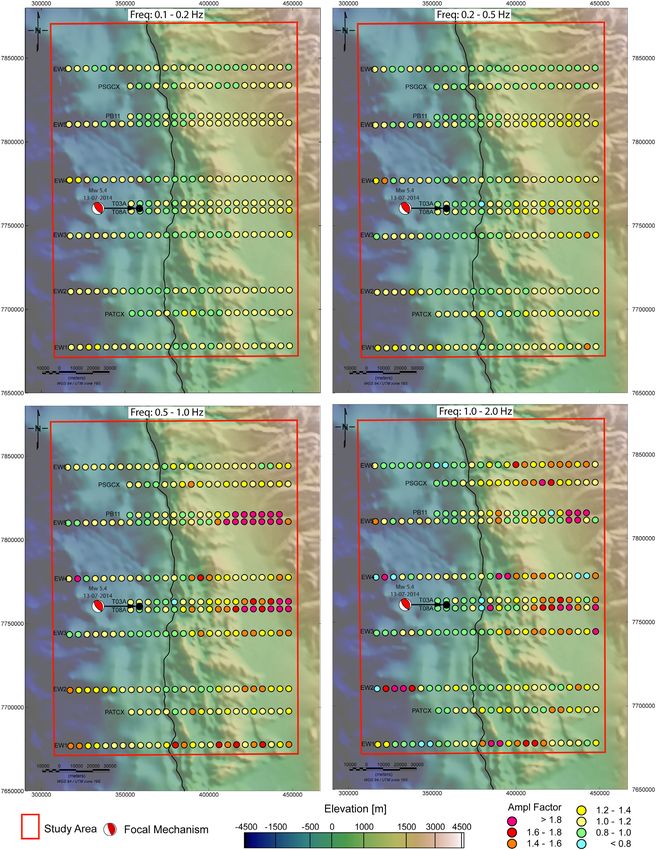
In this work, the results show that basin amplifications are amplitude and complexity of the amplification is intimately related
strongly frequency-dependent and are related to the size of the to the frequency, as is clearly visible in the increasing amplifica-
basin. For example, in the frequency band between 0.1 and 2.0 Hz tion values with the increasing frequency bands for the smaller Alto1158 T. Garcı́a-Pérez et al.
Downloaded from https://academic.oup.com/gji/article/227/2/1143/6316783 by University College London user on 10 August 2021
Figure 11. Map showing the energy amplification ratio in the velocity waveforms between synthetic seismograms obtained using the model with topography
and the model with topography and basins. The map shows coloured circles for each station location, in which the colours represent the calculated amplification
factor with values between < 0.8 and > 1.8. Values above 1 represent relative amplification in the topography and basins model, while values below 1 represent
relative deamplification. The beach ball represents the Mw 5.4 2014 July 13 earthquake and the blue squares represent the basins. The grey-shaded elevation
map shows the geomorphological features related to the coastal cliff and the coastal cordillera to the east of the coastal line (black line).
Hospicio basin. This can be seen as the basin’s size interacting more the height of the basin. This basin-related amplification frequency
with higher frequency waves (Semblat et al. 2002). These results dependency was also shown in several previous empirical and an-
agree with the results of Paolucci & Morstabilini (2006), who found alytical studies (Borcherdt 1970; Borcherdt & Glassmoyer 1992;
that the peak of amplification occurs at frequencies slightly larger Field 1996; Semblat et al. 2002; Day et al. 2008)
than the fundamental resonance frequency of the layer given by Ours results also show deamplification occurring at the edges of
f0 = Vs /4H, where Vs is the S-wave velocity of the basin and H is the basins, probably related to reflected waves that interact with theEffects of topography and basins on seismic wave amplification 1159
Downloaded from https://academic.oup.com/gji/article/227/2/1143/6316783 by University College London user on 10 August 2021
Figure 12. Amplification factor maps for the velocity waveforms between synthetic seismograms obtained using the model with topography and the model
with topography and basins for frequency ranges between 0.1–0.2 Hz, 0.2–0.5 Hz, 0.5–1.0 Hz and 1.0–2.0 Hz. The maps show coloured circles for each station
location, in which the colours represent the calculated amplification factor. Values above 1 represent relative amplification in the topography and basins model,
while values below 1 represent relative deamplification. The beach ball represents the Mw 5.4 2014 July 13 earthquake and the blue squares represent the
basins. The grey-shaded elevation map shows the geomorphological features related to the coastal cliff and the coastal cordillera to the east of the coastal line
(black line).You can also read