Refined estimates of water transport through the Åland Sea in the Baltic Sea
←
→
Page content transcription
If your browser does not render page correctly, please read the page content below
Ocean Sci., 18, 89–108, 2022
https://doi.org/10.5194/os-18-89-2022
© Author(s) 2022. This work is distributed under
the Creative Commons Attribution 4.0 License.

Refined estimates of water transport through
the Åland Sea in the Baltic Sea
Antti Westerlund1 , Elina Miettunen2 , Laura Tuomi1 , and Pekka Alenius1
1 Finnish   Meteorological Institute, Marine Research, Erik Palménin aukio 1, P.O. Box 503, 00101 Helsinki, Finland
2 Finnish   Environment Institute SYKE, Marine Research Centre, Latokartanonkaari 11, 00790 Helsinki, Finland

Correspondence: Antti Westerlund (antti.westerlund@fmi.fi)

Received: 16 June 2021 – Discussion started: 23 June 2021
Revised: 10 November 2021 – Accepted: 12 November 2021 – Published: 19 January 2022

Abstract. Water exchange through the Åland Sea (in the            significant volume of deep water still enters the Åland Sea
Baltic Sea) greatly affects the environmental conditions          through the depression west of the Lågskär Deep. Better
in the neighbouring Gulf of Bothnia. Recently observed            spatial and temporal coverage of current measurements is
changes in the eutrophication status of the Gulf of Both-         needed to further refine the understanding of water exchange
nia may be connected to changing nutrient fluxes through          in the area. Future studies of transport and nutrient dynamics
the Åland Sea. Pathways and variability of sub-halocline          will eventually enable a deeper understanding of eutrophica-
northward-bound flows towards the Bothnian Sea are impor-         tion changes in the Gulf of Bothnia.
tant for these studies. While the general nature of the wa-
ter exchange is known, that knowledge is based on only a
few studies that are somewhat limited in detail. Notably, no
high-resolution modelling studies of water exchange in the        1   Introduction
Åland Sea area have been published. In this study, we present
a configuration of the NEMO 3D hydrodynamic model for             The Gulf of Bothnia, in the northern Baltic Sea, has so far
the Åland Sea–Archipelago Sea area at around 500 m hori-          been in relatively good environmental health and free from
zontal resolution. We then use it to study the water exchange     both seasonal and long-term hypoxia occurring in many other
in the Åland Sea and volume transports through the area. We       Baltic Sea basins. Recently evaluated long-term trends, how-
first ran the model for the years 2013–2017 and validated         ever, show changes in the eutrophication status (Kuosa et al.,
the results, with a focus on the simulated current fields. We     2017), including nutrient and oxygen concentrations. Rea-
found that the model reproduced current direction distribu-       sons for these changes are currently not fully understood.
tions and layered structure of currents in the water column       One piece of the puzzle is the still poorly understood fluxes
with reasonably good accuracy. Next, we used the model to         of nutrient-rich and possibly hypoxic water from the Baltic
calculate volume transports across several transects in the       proper in the south (Ahlgren et al., 2017). The first crucial
Åland Sea. These calculations provided new details about          step on the way to understanding these fluxes is studying the
water transport in the area. Time series of monthly mean vol-     routes of water to and from this area.
ume transports showed consistent northward transport in the          Water has two main routes between the Baltic proper and
deep layer. In the surface layer there was more variability:      the Gulf of Bothnia: the deeper but narrower Åland Sea
while net transport was towards the south, in several years       and the wider but shallower Archipelago Sea (Fig. 1). A
some months in late summer or early autumn showed net             series of sills and smaller sub-basins regulate the exchange
transport to the north. Furthermore, based on our model cal-      in the Åland Sea route, and numerous islands and nar-
culations, it seems that dynamics in the Lågskär Deep are         row passages control the exchange in the Archipelago Sea
more complex than has been previously understood. While           route. Depths in the area vary from just a few metres in the
Lågskär Deep is the primary route of deep-water exchange, a       shallow archipelago area to 300 m in the Åland Sea, with
                                                                  many relatively steep topographic gradients along the bot-

Published by Copernicus Publications on behalf of the European Geosciences Union.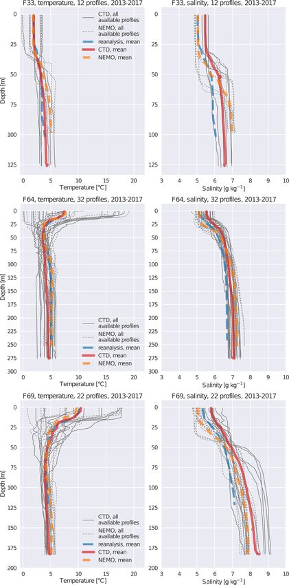
90                            A. Westerlund et al.: Refined estimates of water transport through the Åland Sea, Baltic Sea

Figure 1. (a) Model domain and bathymetry. The main focus area of this study is shown with a rectangle. In addition, several geographic
references are displayed. (b) A more detailed map of the main focus area. Sub-basins and sill areas relevant for the analysis are shown.
Furthermore, the locations of stations and transects mentioned in the text are indicated.

tom (Leppäranta and Myrberg, 2009). The mean depth of the             Åland Sill in the Southern Quark area located at the northern
Archipelago Sea is only 19 m. It is characterized by numer-           edge of the Åland Sea.
ous small islands and narrow straits.                                    Complex bathymetric features, significant depth varia-
   The Åland Sea has two basins. The smaller Lågskär Deep             tions and patchy observational data pose challenges for
(also known as the Lågskär Basin or southern Åland Sea                studying the exchanges between the Baltic proper and the
basin) has a maximum depth of 220 m, and the larger                   Gulf of Bothnia. Likewise, previous modelling efforts have
Åland Sea proper (or the northern Åland Sea basin) has a              been hindered by insufficient local resolution and unresolved
maximum depth of 301 m. Three sills affect water exchange             bathymetric features. In this paper, we present a new high-
through the Åland Sea. The southernmost of these is the               resolution three-dimensional hydrodynamic modelling con-
Southern Åland Sill, which is a narrow channel on the south-          figuration for the Åland Sea and the Archipelago Sea. This
ern edge of the Åland Sea. It is a major barrier for deep water       configuration provides a platform for studying this region.
entering from the Baltic proper. Next is the Åland Sea Middle         We focus on the Åland Sea to investigate the exchange fluxes
Sill between Söderarm and Lågskär, separating the Lågskär             through the area.
Deep from the Åland Sea proper. The third is the Northern                The first comprehensive study of water exchange between
                                                                      the Baltic proper and the Gulf of Bothnia was probably that

Ocean Sci., 18, 89–108, 2022                                                                 https://doi.org/10.5194/os-18-89-2022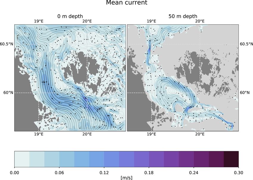
A. Westerlund et al.: Refined estimates of water transport through the Åland Sea, Baltic Sea                                   91

of Witting (1908). In the early 1920s, Åland Sea studies were     that transport estimates had significant uncertainty and de-
continued through Finnish–Swedish co-operation, with both         pended on the choice of averaging timescales for velocities
hydrographic and current meter observations taken in 1922         and transports and on the chosen locations of the cross sec-
and 1923. Several hydrographic surveys were conducted in          tions used for inflow and outflow estimates.
the Åland Sea in the 20th century (e.g. Lisitzin, 1951). In          The main aim of this paper is to investigate modelled
the late 1950s Hela (1958) estimated the water exchange be-       routes of water through the target area with a high-resolution
tween the Gulf of Bothnia and the Baltic proper using hy-         model configuration. We also study their variability on a
drographic data from the area measured in 1956. As was            monthly scale and evaluate the reliability of the estimates.
already described by Granqvist (1938) for example, Hela           This information will provide the basis for future studies of
(1958) found that there were no clearly defined water masses      transport dynamics in the area and serve as the first step for
and that continuous mixing occurs between waters of differ-       future investigations, which will enable us to understand why
ent origins. Hela (1958) nevertheless presented TS diagram        and how the eutrophication status in the Gulf of Bothnia is
analysis (calling it in this case “schematic and more or less     changing.
arbitrary”), which he used to identify a deep-water type orig-       Our modelling configuration is based on the NEMO model
inating from water entering from the Baltic proper. The term      core (Madec and NEMO System Team, 2019), which has
“deep water” was used to emphasize that this water was not        previously been applied at high resolution in the nearby
Baltic proper bottom water, as the most saline bottom water       Gulf of Finland (Vankevich et al., 2016; Westerlund et al.,
is not able to flow over the Southern Åland Sill. Also notable    2018, 2019). The Archipelago Sea has been previously mod-
were the warm water lenses below the thermocline and above        elled at high resolution by Tuomi et al. (2018) and Miettunen
the temperature minimum, which Hela (1958) analysed to be         et al. (2020), who used the COHERENS model (Luyten,
warm-water intrusions from the Baltic proper. This analysis       2013). The configuration presented in this study builds on
was later further elaborated by Hela (1973).                      that experience, but also covers the Åland Sea, which was not
   Palosuo (1964) evaluated the water exchange using bathy-       included in the COHERENS setup. In their study Tuomi et al.
metric information to study the channels and sill depths on       (2018) found that the σ coordinates used in the COHERENS
the deeper paths leading from the Baltic proper to the Gulf       implementation introduced over-mixing, especially in deep
of Bothnia through Lågskär Deep and the Åland Sea. He             channels where there were large depth gradients from one
also concluded from data from station F69 that at Lågskär         grid point to the next. To mitigate this issue, we chose the
Deep there is large variability in the salinity in the surface    z∗ vertical coordinate system for our implementation. This is
layer up to 80–90 m depth, below which salinity increases         a geopotential vertical coordinate system where sea surface
constantly to values up to 8 g kg−1 . The Åland Sea proper        height variations are distributed over the whole water column
showed similar salinity variation at the surface layer and        (e.g. Klingbeil et al., 2018). It has been successfully applied
more constant values in the deeper layers, being less saline      in the aforementioned Gulf of Finland configuration, as well
than in the Lågskär Deep. A constant northward current was        as in regional configurations (Hordoir et al., 2019).
estimated to be present in the deeper layer of the Åland Sea         Bathymetric features greatly affect water exchange in this
proper based on the datasets in both Palosuo (1964) and Hela      topographically complex and irregular area. Forming a cor-
(1958).                                                           rect understanding requires detailed information about ex-
   After these studies, the most recent in-depth investigations   change pathways and sill depths, for example. In principle,
concentrating on the water exchange in the Åland Sea were         bathymetric data are available from different sources with
produced within the framework of the Finnish–Swedish co-          high spatial resolution; see, e.g. the Baltic Sea Bathymetry
operation to investigate the environmental condition of the       Database (BSBD), available at http://data.bshc.pro (last ac-
Gulf of Bothnia in the 1970s (Ehlin and Ambjörn, 1977; Am-        cess: 4 January 2022), or the European Marine Observa-
björn and Gidhagen, 1979).                                        tion and Data Network (EMODnet) bathymetry, available
   These earlier studies relied heavily on observational and      at https://www.emodnet-bathymetry.eu (last access: 4 Jan-
mostly short-term datasets. More recently, numerical mod-         uary 2022). However, the resolution and accuracy of the
elling has made it possible to study currents and water ex-       source data are not equally good in all areas; see, e.g. Jakob-
changes fully in four dimensions, giving us spatial and tem-      sson et al. (2019) for an example from the Åland Sea. For
poral coverage not possible with just observations. This al-      this paper, we took a significant effort to ensure that bathy-
lows us to investigate intra- and inter-annual variability, for   metric features in key areas are represented as realistically as
example, with much richer detail than we could with obser-        possible in the model.
vations alone.                                                       In this paper, we first introduce the new modelling config-
   Modelling studies investigating transports in this area have   uration. Following this, as this is the first time such a high-
so far been rare. A notable exception is a study by Myrberg       resolution model has been applied to the Åland Sea, a val-
and Andrejev (2006). Although they concentrated mainly on         idation of a 5-year model run is carried out. After that, we
the Gulf of Bothnia as a whole, they also looked at water ex-     investigate modelled currents and finally study volume trans-
change in the Åland Sea–Archipelago Sea area. They found          ports through the study area. These results are then compared

https://doi.org/10.5194/os-18-89-2022                                                             Ocean Sci., 18, 89–108, 2022
92                           A. Westerlund et al.: Refined estimates of water transport through the Åland Sea, Baltic Sea

to earlier estimates, and future directions for research are        along the transects to investigate the pathways of water more
charted.                                                            closely.

                                                                    2.2   Bathymetric data
2     Materials and methods
                                                                    We compiled the model bathymetry from two sources.
2.1    Modelling methods                                            The primary source for bathymetric data was the VELMU
                                                                    (Finnish Inventory Program for the Marine Environment)
We set up the NEMO three-dimensional hydrodynamic                   bathymetry model (Finnish Environment Institute), which
model version 4.0.3 for the Åland Sea and the Archipelago           covers the Finnish Exclusive Economic Zone (EEZ). For the
Sea at 0.25 nmi (nautical mile) or approximately 500 m hor-         part of the model domain that is outside the Finnish EEZ,
izontal resolution. Model domain and bathymetry are de-             we used the BSBD from the Baltic Sea Hydrographic Com-
picted in Fig. 1. The modelled time span covered June 2012          mission, which covers the whole modelling domain. The res-
to December 2017, but in our analysis we concentrate on re-         olution of the VELMU bathymetry model is approximately
sults starting from January 2013 to ensure that the model had       20 m, but the resolution of its source data is not as high in all
a long enough initialization period.                                locations. The same applies to any other gridded bathymetry
   The model setup used the z∗ vertical coordinate system.          dataset. The bathymetry data for the 0.25 nmi model grid was
There were 200 vertical levels. Level thickness increased           compiled by calculating the mean of VELMU depth points
slightly with depth, being 1 m at the surface and 1.1 m at          in each model grid point. BSBD data has a resolution of
120 m depth. Below the depth of 120 m, the thickness in-            0.25 nmi in the Åland Sea.
creased more rapidly to about 8 m at the very bottom. This             The bathymetric source datasets have mostly been created
arrangement allowed for the top part of the water column to         and interpolated automatically. In addition, the model grid
be resolved at a relatively high resolution while keeping the       was compiled from those datasets automatically, resulting in
number of levels manageable.                                        a somewhat patchy grid. For example, the channels crossing
   Horizontal viscosity was parameterized with the                  the area were not all continuous or deep enough, the sills
Smagorinsky formulation (Smagorinsky, 1963). Smagorin-              were typically too shallow, and there were some very steep
sky formulation has been a popular choice for studying              depth gradients challenging for the hydrodynamic model. To
nearby sea areas; see, e.g. Zhurbas et al. (2008). In the           mitigate these issues, we checked and edited the model grid
vertical, we used the GLS (generic length scale) mixing             manually to ensure that it represented topographic features in
scheme configured to produce the k- model. This parame-            the area as accurately as possible in the 0.25 nmi resolution.
terization has previously been successfully applied in Baltic          The most crucial places to be modified were the sills
Sea NEMO configurations (e.g. Hordoir et al., 2019; West-           and channels that control the water exchange through the
erlund, 2018), and it has been able to reproduce seasonal           Åland Sea. Each sill area (locations indicated with magenta
stratification in the Bothnian Sea quite well (Westerlund and       in Fig. 1) and its surroundings were checked manually and
Tuomi, 2016).                                                       edited to equal the known sill depths. The channels in the
   We used a sea ice model with a thermodynamic formula-            southern and northern parts of the Åland Sea were also edited
tion (as was previously done for the Gulf of Finland by West-       to be continuous at a certain depth and overall wide enough
erlund et al., 2018, 2019). This somewhat eased the relatively      (at least 3–4 grid points) so that they would enable appropri-
high computational requirements of this configuration. Dur-         ate water flow between the basins.
ing our study period, the ice seasons in the Baltic Sea area           Finally, the modified model depth grid was filtered with a
were mostly mild or very mild. In the Åland Sea, within our         Gaussian filter with a standard deviation of 1.2 grid points
modelling period there was a notable amount of ice only dur-        to smooth out the steepest bathymetry gradients and ensure
ing winter 2012–2013, which has been classified as an aver-         numerical stability.
age ice season by the FMI (Finnish Meteorological Institute).
The winter of 2017/2018 was also an average ice season, but         2.3   Forcing and boundary conditions
the ice in the area formed only after our modelling period.
   We saved 6 h averages of 3D temperature, salinity and cur-       We subset the meteorological forcing from the ERA5 atmo-
rent fields. Sea surface height was recorded at 1 h intervals,      spheric reanalysis provided by Copernicus Climate Change
while volume transports were saved once a day. We com-              Service (Hersbach et al., 2018). We used hourly 10 m winds,
puted volume transports from the model for a number of tran-        2 m air temperature, 2 m dew point temperature, mean sea
sects. These were integratedRR over theRRwhole transect to cal-     level pressure, precipitation, snowfall rate, shortwave radia-
culate a time series: Fv = v dA = v dzdl. Here v is the             tion flux and longwave radiation flux fields from the reanal-
velocity across the transect, A is the area of the transect, z is   ysis to force the model.
the depth along the transect and l is the length of the transect.
                                                          R            The model configuration had open boundaries to the Both-
We also calculated volume transports per unit length ( v dz)        nian Sea in the north and the Baltic proper and the Gulf

Ocean Sci., 18, 89–108, 2022                                                              https://doi.org/10.5194/os-18-89-2022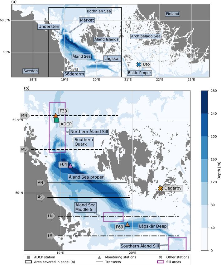
A. Westerlund et al.: Refined estimates of water transport through the Åland Sea, Baltic Sea                                    93

of Finland in the south. We took lateral boundary con-
ditions and initial conditions for the model from a re-
gional reanalysis configuration (Baltic Sea Physical Reanaly-
sis Product BALTICSEA_REANALYSIS_PHY_003_011)
provided by the Copernicus Marine Environment Monitoring
Service (CMEMS). Initial conditions consisted of interpo-
lated salinity and temperature fields. Boundary conditions in-
cluded Flather radiation conditions for sea surface heights at
one hour intervals and barotropic velocities at 24 h intervals.
FRS (flow relaxation scheme) boundary conditions were ap-          Figure 2. Sea surface height at the Föglö Degerby tide gauge in
plied for temperature and salinity at 1 d intervals. A no-flux     2017, showing a comparison between measurements and the model.
condition was applied for the small open-sea segment at the
south-east edge of the model domain, which improved the
                                                                   data has been quality checked, leaving gaps in the dataset.
stability of the configuration. This area is quite shallow and
                                                                   These gaps due to bad or missing data occurred mainly in
far away from the area of interest in this study, and thus a
                                                                   the upper 40 m layer during spring and summer. On average,
no-flux condition was deemed sufficient for this purpose.
                                                                   33 % of the ADCP measurements were missing in the upper
   There are eight rivers inside the model domain, all of
                                                                   layer, but some months lacked up to 77 % of measurements.
which are on the Finnish coast. We took daily values of
                                                                   If a 6 h time slot over which the means were calculated was
river discharge from the watershed model VEMALA which
                                                                   missing more than 50 % of the measurements, we discarded
is an operational, national-scale nutrient loading model for
                                                                   the time slot both from the averaged ADCP data and from
Finnish watersheds (Huttunen et al., 2016).
                                                                   the model data when calculating the bias and current roses.
2.4   Observational data
                                                                   3     Results
We used sea surface height from the Föglö Degerby station
(see Fig. 1). There are also two other tide gauges within the      3.1     Model validation
model domain in Turku and Forsmark. However, we did not
use data from these sites as they are not representative of        3.1.1    Sea surface height
the overall sea level variation in the study area but instead
reflect local effects. The Turku tide gauge is located in the      Adequate accuracy of major sea surface height (SSH) vari-
inner archipelago on the Finnish coast, and the Forsmark tide      ations is an indication that the model is able to reproduce
gauge on the Swedish coast is set up in a constructed area to      barotropic dynamics reliably. While the model configuration
monitor water levels for a nuclear power plant.                    in this study has not been built for sea level forecasting, a
   We also investigated temperature and salinity profiles from     comparison of modelled sea surface height with tide gauge
three stations in the Åland Sea: F33, F64 and F69 (see Fig. 1).    data gives a quick overview of overall model performance.
These sites are sampled more often, and their temporal cov-        The range of sea level variability and the timing of events are
erage is better than in other stations in the area. However, the   both important when considering the suitability of the model
number of profiles is still quite modest, and we supplemented      for the study at hand. However, it is good to bear in mind
them with data from the Utö intensive monitoring station at        that these results are heavily dominated by how well SSH
the southern edge of the Archipelago Sea.                          is presented in the boundary conditions. Furthermore, as the
   We used current measurement data from a location near           vertical reference for sea level differs between model and tide
the station F33 to study how the model is able to repro-           gauge data, comparison of bias is not feasible.
duce observed currents (station “ADCP” in Fig. 1). The                The results from the Föglö Degerby station (see Fig. 1)
measurements were carried out with a bottom-mounted                showed that the model was able to reproduce sea level vari-
300 kHz Workhorse Sentinel acoustic Doppler current pro-           ations quite well. A part of the SSH time series is displayed
filer (ADCP). The location was 126 m deep, and the corre-          in Fig. 2 showing typical results. Most importantly, it shows
sponding model grid point was 110 m deep. The measure-             that the timing of sea level events is quite accurate. There are
ments ranged vertically from 8 m depth down to 112 m depth         a few cases where the magnitude of the event was incorrectly
at 2 m intervals. This dataset covers the period of 6 August       estimated in the model, although in most cases the differ-
2016–3 July 2018 with a time interval of 30 min.                   ences were quite small. It is also significant that the range
   The modelled current components were saved as means of          of water level variability is well represented overall. For this
6 h. For the comparison between the measured and modelled          station in 2017, the correlation coefficient for the modelled
currents, we first calculated the 6 h means of the measured        and observed time series was 0.85, and the standard devia-
horizontal current components and then from these means,           tion of the observed and modelled values differed less than
calculated the current magnitude and direction. The ADCP           3 cm.

https://doi.org/10.5194/os-18-89-2022                                                              Ocean Sci., 18, 89–108, 2022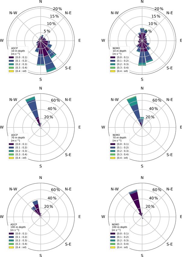
94                           A. Westerlund et al.: Refined estimates of water transport through the Åland Sea, Baltic Sea

3.1.2   Temperature and salinity

The vertical structure of the water column is illustrated
with observed and modelled temperature and salinity profiles
from three monitoring stations (F33, F64 and F69) in Fig. 3,
which shows all available profiles from these stations along
with overall mean profiles. In addition, we compared profiles
individually to model data to get an overview of model per-
formance. For the study at hand, the ability of the model to
estimate the vertical position of the halocline and thermo-
cline correctly is of interest. For example, if the halocline
was continuously and severely misplaced in the model, that
would likely indicate problems for volume transport calcula-
tions.
   Vertical temperature profiles were generally quite well re-
produced. This includes the strength of the thermal stratifica-
tion and its vertical position, which were relatively correctly
estimated. Salinity profiles revealed that salinity biases are
most prevalent near the surface, with typical differences up
to 1 g kg−1 above the halocline. Halocline depth in the model
was mostly reasonable and the errors in individual profiles
were similar to the ones visible in the means. There are some
individual profiles, where the model was clearly unable to
capture the dynamical situation correctly and where there
were errors of 10 or even 20 m in halocline depth. Further-
more, in some cases the shape of the profiles suggested sub-
mesoscale activity, which is very difficult to fully model due
to the chaotic nature of such phenomena. Overall, the moder-
ate availability of profile data from the modelling area some-
what limits the conclusions that can be drawn based on this
data. For instance, almost all profile data available from these
stations have been measured in January, May or August. All
in all, the ability of the model to reproduce vertical temper-
ature and salinity structure seems to be well within expected
accuracy for a state-of-the-art model and the area of interest.
   In addition to this, we inspected temperature and salin-
ity time series from the Utö intensive monitoring station at
the southern edge of the Archipelago Sea (not shown). Over-
all, these results indicated very similar model skill to what
has previously been reported for the NEMO model in nearby
sea areas (see, e.g. Westerlund and Tuomi, 2016; Westerlund
et al., 2018). Temperature evolution was quite well repro-         Figure 3. Temperature and salinity profiles from three monitoring
duced at all depths and seasons, although there were larger        stations 2013–2017. All available measurement profiles and corre-
differences deeper in the water column. While the frequency        sponding modelled profiles are shown, along with their means. In
of the observations did not allow for a detailed analysis of       addition, the mean of the profiles taken from the reanalysis product
                                                                   used as a boundary condition for the model is shown. Please note
short-term variability, it does seem that at least some shorter-
                                                                   that the number of profiles varies from station to station.
term events are also reproduced by the model. Salinity obser-
vations did not show the same kind of short-term variability
as the modelled time series. The general level of modelled         3.2     Analysis of currents
salinity values was quite reasonable.
                                                                   3.2.1    Simulated and measured currents in the
                                                                            Southern Quark

                                                                   To evaluate the quality of modelled currents, we compared
                                                                   modelled current magnitudes and directions with observa-

Ocean Sci., 18, 89–108, 2022                                                              https://doi.org/10.5194/os-18-89-2022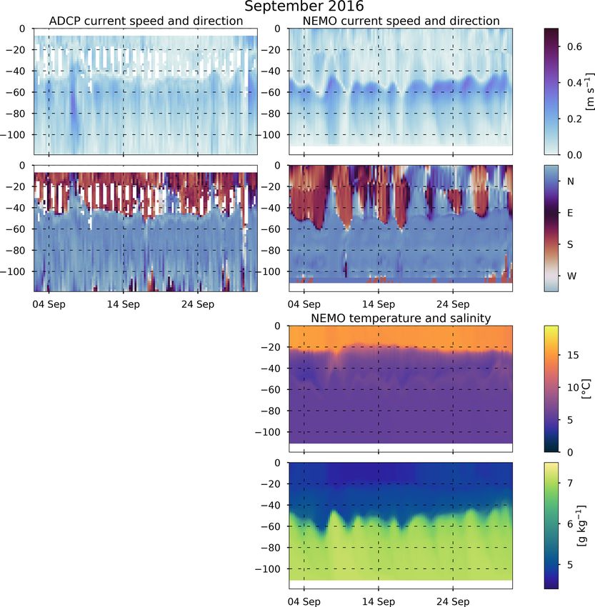
A. Westerlund et al.: Refined estimates of water transport through the Åland Sea, Baltic Sea                                   95

Figure 4. Current magnitudes and directions in September 2016 as measured at the ADCP station and as seen by the model. Modelled
temperature and salinity profiles are also displayed.

tions at the ADCP installation (location shown in Fig. 1).        As we consider mainly current dynamics and transport anal-
Both model and ADCP data were available for the period            ysis, the changes of properties occurring at the halocline are
of August 2016–December 2017. While time- and space-              more significant than those at the thermocline, for example
averaged currents saved from the model often represent dif-       those regarding the direction distribution of currents. For this
ferent things than the very local observations from ADCP in-      reason, we use “upper” or “surface layer” to signify the layer
struments, they can still be used to get an overview of model     above the halocline and “lower” or “deep layer” to signify
performance in the area where the ADCP was located.               the layer below it. We specifically state each time when the
   The vertical profiles of modelled currents had a similar       intermediate layer is being considered.
structure as the measured currents. During autumn and win-           Modelled current magnitudes were highest in the surface
ter, there were two layers: an upper layer above the perma-       layer of a few metres and just below the halocline at depths
nent halocline and a deep layer below the halocline (Fig. 4).     of 50–70 m. The strongest currents occurred typically in late
During the thermally stratified period, three different layers    autumn or winter. In the upper layer above the halocline,
were visible: a surface layer above the thermocline, an inter-    the monthly mean current magnitudes varied from 0.09–
mediate layer between the thermocline and the halocline, and      0.20 m s−1 in the surface to 0.05–0.15 m s−1 at the depths
a deep layer below the halocline. The surface layer was more      of 10–40 m. At depths of 50–70 m, the monthly means var-
easily visible in modelled current profiles than in measure-      ied from 0.11 to 0.23 m s−1 ; the highest monthly mean was
ments, as the ADCP data was missing the upmost 8 m layer.         seen at 60 m depth in February 2017. In the lower parts of
The depth of the thermocline in the model mainly undulated        the water column, there was less seasonal variation in cur-
between 10–25 m and the depth of the halocline between 40–        rent magnitudes and the monthly mean current magnitudes
70 m (Fig. 4). ADCP current speed and direction data showed       decreased with depth from 0.08–0.12 m s−1 at 80 m depth to
that observed halocline depth was mainly between 40–60 m.

https://doi.org/10.5194/os-18-89-2022                                                             Ocean Sci., 18, 89–108, 2022
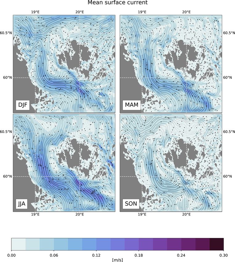
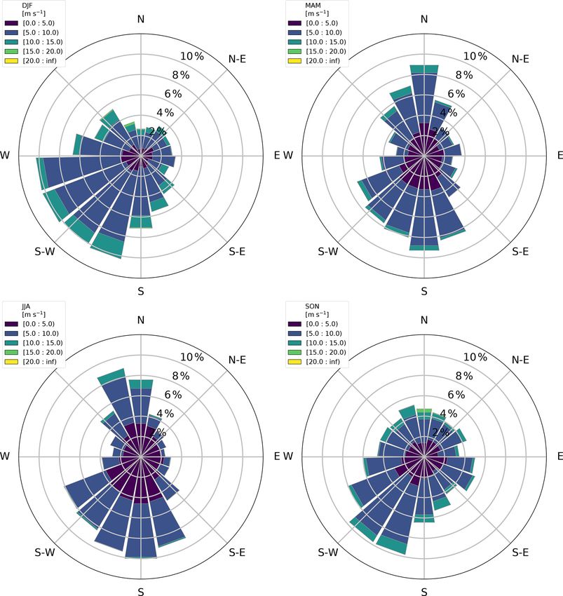
96                          A. Westerlund et al.: Refined estimates of water transport through the Åland Sea, Baltic Sea

Figure 5. Bias and RMSE in the modelled U (zonal) and V (meridional) current components and current magnitude at the ADCP station
from August 2016 to December 2017.

0.004–0.013 m s−1 at 110 m depth (representing the deepest         the modelled currents was towards the south, but the fraction
model layer at the ADCP station coordinates).                      of northward currents was larger than in the measurements,
   To validate the modelled currents, we calculated bias and       i.e. 26 % of the whole comparison period.
root-mean-square error (RMSE) in the modelled horizontal              In the lower layer, there was less variation in the current di-
current components and the current magnitude for the period        rections than in the upper layer. For example, at 70 m depth
of August 2016–December 2017. In general, the U (zonal)            the measured and modelled currents were mainly directed to-
component was underestimated in the upper 30 m and over-           wards north–north-west, but the modelled currents showed a
estimated below that, whereas the V (meridional) component         larger fraction of currents over 0.20 m s−1 than the observa-
was mainly overestimated above 90 m depth and underesti-           tions (Fig. 6). At 100 m depth, the observed currents were di-
mated below that (Fig. 5). The bias in the current magnitude       rected towards the north-west and north–north-west, whereas
was small near the surface, increased towards the halocline        the modelled current direction was dominantly towards the
and decreased again below the halocline. The largest bias          north–north-west. As the current direction at this depth fol-
and RMSE in the current magnitude occur at depths of the           lows the bottom topography, this difference between the ob-
halocline, with values up to 0.061 and 0.145 m s−1 , respec-       served and modelled current direction is possibly caused by
tively. In the lower parts for the water column, the bias in       small differences between the real bottom topography and
magnitude was negative, being −0.051 m s−1 at the depth of         the model bathymetry.
112 m, because the model grid point is shallower than the
ADCP measurement site.                                             3.2.2   Seasonality of currents in the Åland Sea
   Both in measured and modelled currents, the dominant
current direction was towards the southern sector (SW–SE) in       To study the seasonality of circulation patterns both in the
the upper layer and towards the northerly sector (NW–NE) in        surface layer and deeper in the water column, we calcu-
the lower layer. However, the currents in the upper layer had      lated the mean current field over the period of January 2013–
more variation in direction, and northward-flowing currents        December 2017 (Fig. 7) and the seasonal mean current fields
also occurred. In the model, these northward currents were         (Fig. 8). In addition, seasonal wind roses from the ERA5
vertically more uniform and lasted for longer periods than in      forcing at Märket were inspected (Fig. 9). Winter was de-
the measurements. Moreover, the model showed northward             fined to be from December of the previous year to February
currents at times when the observed current direction was          (DJF), spring was from March to May (MAM), summer was
southward. For example, at 10 m depth the measured current         from June to August (JJA) and autumn was from September
directions were mainly towards south and south-east, and the       to November (SON).
fraction of northward currents (towards sectors NW–NE) was            During 2013–2017, the winds at Märket area were most
small, 11 % of the whole comparison period August 2016–            frequent from the W–SSW sector in winter seasons and from
December 2017 (Fig. 6). The prevailing current direction in        SW–SSE and N in spring and summer seasons. In autumn

Ocean Sci., 18, 89–108, 2022                                                             https://doi.org/10.5194/os-18-89-2022
A. Westerlund et al.: Refined estimates of water transport through the Åland Sea, Baltic Sea                                   97

Figure 6. Comparison between measured and modelled currents at the ADCP location. Current roses are shown for 6 August 2016–28
December 2017 at depths of 10, 70 and 100 m. Please note that current roses indicate the direction where the currents flow to.

seasons, the most frequent wind direction was from SW, but        in the surface layer were stronger at the western side of the
the directional distribution in the wind rose is otherwise even   basin than at the eastern side.
higher than in the other seasons.                                    Autumn was the season with the largest inter-annual vari-
   Looking at the surface currents, all the seasonal means        ation in current directions, but the southward and south-
showed southward currents through the Åland Sea turn-             eastward currents were still dominant in most years. To put
ing south-eastward or eastward in the southern part of the        it differently, the persistency of surface currents was signif-
Åland Sea (Fig. 8). In the eastern side of the Åland Sea, a       icantly lower in autumn than in other seasons. This is likely
characteristic feature was a anticlockwise loop existing in au-   related to the significant inter-annual variability in wind di-
tumn, winter and spring. Its location has both seasonal and       rections during autumn. In summer and spring, there was
inter-annual variation. In general, the mean current speeds       very little year-to-year directional variation in winds and sur-

https://doi.org/10.5194/os-18-89-2022                                                             Ocean Sci., 18, 89–108, 2022
98 A. Westerlund et al.: Refined estimates of water transport through the Åland Sea, Baltic Sea
Figure 7. Modelled mean currents at the surface and 50 m depth in 2013–2017.
face currents. This is visible in the lengths of the vectors in channels and also higher on the eastern side than on the west-
the seasonal mean figure. Although current magnitudes were ern side of the loop in the Åland Sea proper.
not significantly smaller in autumn, the mean current vectors
are still shorter just because of the component-wise averag- 3.3 Volume transports in the Åland Sea
ing of current vectors.
While most seasons generally had southward currents in To better understand water exchange in the Åland Sea, we
the Åland Sea, winter 2013–2014 was somewhat exceptional. analysed volume transports along six zonal (west–east) sec-
During that time, the wind direction at Märket was mainly tions across the basin (locations shown in Fig. 1). For this
from the sector between SW and SE, and the surface currents analysis, transports were integrated over the upper part of the
were northward or north-eastward almost in the whole model water column down to 40 m depth, over the lower part of the
domain. Winter 2012–2013 showed a large variation in wind water column below 40 m depth and over the whole water
directions, the prevailing direction being from NE, while in column. This roughly split the water column into an upper
winters from 2014–2015 onward the prevailing wind direc- (and intermediate) layer above the halocline and a deep layer
tion was from SW or W. The strongest southward currents in below the halocline (cf. Sect. 3.2.1). While the depth of the
winter can be seen in 2016–2017 when the wind distribution halocline varies somewhat spatially and temporally, the salin-
was weighed more to westerlies and the portion of souther- ity profiles and ADCP data suggest that 40 m is a reasonable
lies was lower than on average. estimate for this analysis. As our main interest is in the sub-
Deep-layer currents showed less seasonal variation in di- halocline deep-water transports, and as analysis of currents
rection than surface currents, and the current direction was revealed some significant current speeds in the model layers
generally northward in all seasons. Figure 7 shows the mean just below the halocline, we deemed it was more important
circulation at 50 m depth as an example. In the southern part to choose a separating depth for the analysis that for the most
of the model domain, the mean current direction was north- part was either at the halocline or slightly above it.
ward and north-westward along the channel that leads to the The locations of the transects (see Fig. 1) were chosen to
Lågskär Deep. In the Åland Sea proper, there was a anti- support the aim to study the deep-layer transports in partic-
clockwise loop covering the whole basin, with stronger cur- ular. Starting from the north, the two northernmost transects
rents on the eastern side of the basin. In the northern part of were set north from Märket and Understen and close to them
the basin, the currents continued northward along the South- on both sides of the sill to capture fluxes across the Northern
ern Quark, and the bathymetry steered the currents north- Åland Sill. The third and fourth transects represent approxi-
eastward near the northern edge of the model domain. The mately the middle and southern part of the Åland Sea proper
persistency of the current direction was high in the narrow to explain the internal dynamics of the Åland Sea. The fifth
and sixth transects are located at the northern and southern
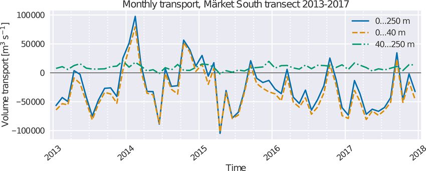
Ocean Sci., 18, 89–108, 2022 https://doi.org/10.5194/os-18-89-2022A. Westerlund et al.: Refined estimates of water transport through the Åland Sea, Baltic Sea 99 Figure 8. Seasonal means of modelled surface currents in 2013–2017. Please note that the means of current vectors are calculated as the means of elements in the vector, not as means of magnitudes. This means that in autumn (SON) when current stability is low, magnitudes of mean vectors (shown) are much smaller than means of magnitudes (not shown). edge of the Lågskär Deep to investigate transports in and out An overview of the modelled transports is consistent with of this area in order to explain the role of the Lågskär Deep the general knowledge of the water exchange in the area. The in the water exchange and eventually in the mixing processes deep-layer transport goes to the north, and the upper-layer of waters coming from the Baltic proper. transport goes on average to the south. Transport in the upper A time series of monthly mean volume transports inte- layer is much larger than in the lower layer and it dominates grated over the whole transect is shown for the Märket South the integrated transport. This can be expected, as water en- transect in Fig. 10. While this time series plot is shown here tering the Gulf of Bothnia from the south must at some point for one transect only, the other transects also show monthly also exit the gulf towards the south and net precipitation (pre- values that are generally of the same order as the ones in cipitation minus evaporation) in this area is close to zero or this Figure. In the upper layer and for the whole water col- slightly positive (cf. Rutgersson et al., 2001). Furthermore, umn, the time series for different transects were highly cor- fresh river runoffs into the Gulf of Bothnia leave the basin related. For example, when comparing the upper-layer time in the surface waters, further increasing the surface transport series for the MS and LS transects, the correlation coefficient towards the south. There were, however, months when the was 0.96. For the lower layer, there was more variance in the overall transport is towards the north, most notably in au- monthly values between transects, and correlation is weaker tumn. The largest values of water transport towards the south when transects are further apart. occurred in late spring and early summer. https://doi.org/10.5194/os-18-89-2022 Ocean Sci., 18, 89–108, 2022
100                          A. Westerlund et al.: Refined estimates of water transport through the Åland Sea, Baltic Sea

Figure 9. Seasonal wind roses in December 2012–November 2017, drawn from the ERA5 winds at the location of Märket weather station.
Please note that wind roses indicate the direction where the wind is blowing from.

Figure 10. Time series of modelled monthly mean volume transports through the Märket south transect near the northern edge of the
Åland Sea 2013–2017. Positive values indicate northward transport. Values for the whole water column, the upper water column up to 40 m
and the lower water column below 40 m are shown.

   Variability from single month to another and single year           note, however, that the high variability of transports means
to another is significant. The mean volume transports for             that the mean transports are very sensitive to the choice of the
the MS transect for the whole modelling period were                   calculation interval. For example, if we had decided to leave
−24 000 m3 s−1 (whole water column), −33 000 m3 s−1 (up-              the somewhat anomalous years 2013 and 2014 out of the cal-
per layer) and 9200 m3 s−1 (lower layer). It is important to          culation for the volume transports, the means for the whole

Ocean Sci., 18, 89–108, 2022                                                                https://doi.org/10.5194/os-18-89-2022
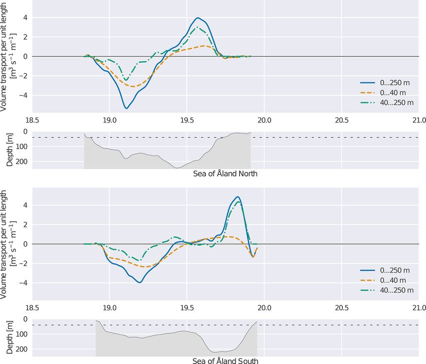
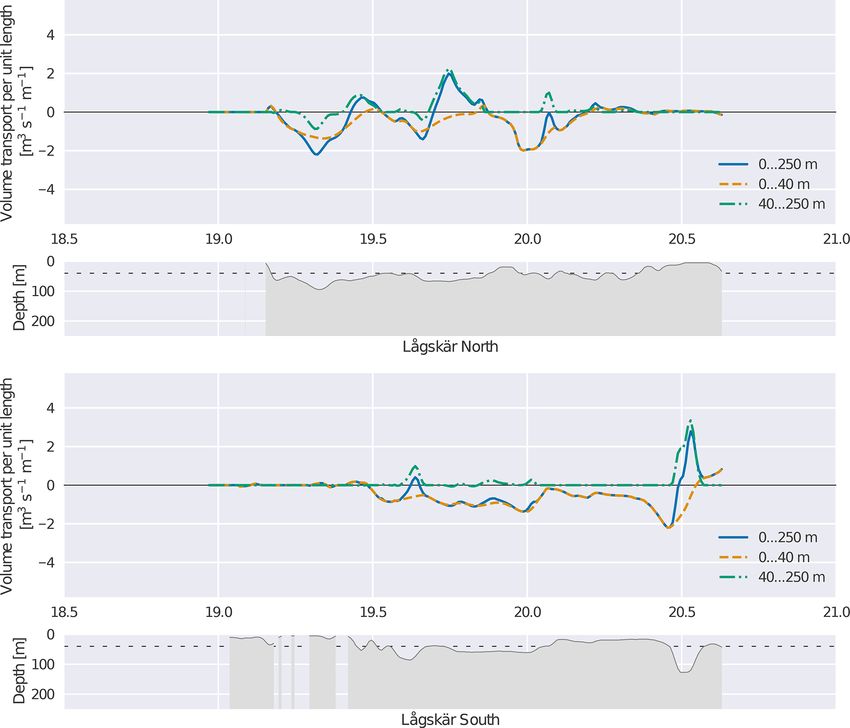
A. Westerlund et al.: Refined estimates of water transport through the Åland Sea, Baltic Sea                                          101

Figure 11. Volume transports per unit length along a transect, integrated over depth, from two northernmost longitudinal transects in the
Åland Sea (MN and MS). Mean values for 2013–2017 shown. Positive values indicate northward transport. Values for the whole water
column, the upper water column up to 40 m and the lower water column below 40 m are shown. In addition, for each transect a depth profile
along the transect is displayed, with the 40 m threshold marked with a dashed line. For reference, 1◦ longitude is here approximately 55 km
in length.

water column would have been 30 %–40 % higher. The lower                is also much larger in the east than in the west. Finally, for
variability of the lower-layer transport means it is much less          the northernmost parts we see deep water flowing northwards
sensitive to the choice of the averaging interval (difference in        between Understen and Märket over the Northern Åland Sill
this case under 6 %).                                                   to the Southern Quark Strait.
   Next, to illustrate the pathways of water, we calculated                These transects also reveal some interesting details about
volume transports per unit length along these six sections              the transports. For example, in the southernmost transect we
(Figs. 11–13). Mean values were calculated for the whole                see that, in addition to the strait located at approximately
study period. Starting now from the south and moving to-                20.5◦ E, some deep water also enters the basin through the
wards the north, waters enter the deep layer in the Lågskär             depression at 19.6◦ E at the south-west corner of the Lågskär
Deep from the Baltic proper mainly across the Southern                  Deep. The primary route is on average responsible for 75 %
Åland Sill through the passage starting east of Bogskär (lo-            of the transport. The rest flows through the western parts of
cated south of the southern edge of our domain) and connect-            the transect.
ing to the south-east corner of the Lågskär Deep. The water                Furthermore, at the northern edge of the Lågskär Deep, the
then is transported to the Åland Sea proper mainly over the             deep-water transport is divided through three different routes.
Åland Sea Middle Sill between Söderarm and Lågskär.                     Transport through the passage east of Lågskär at approxi-
   In the Åland Sea proper, we see a structure where waters             mately 20.1◦ E seems minor when compared to the trans-
flow northwards in the eastern side of the basin and south-             port west of Lågskär and east of Söderarm between 19.3 and
wards in the western side of the basin. Unlike for the other            20.0◦ E. Between Lågskär and Söderarm, deep water can take
parts of the Åland Sea, in this case there is also clear south-         two different routes, and our model indicates that the major-
wards transport in the lower part of the water column in the            ity of flow takes place through the eastern route at approxi-
western part of the transect. This is in line with the loop vis-        mately 19.7◦ E.
ible in this area in Fig. 7. As the eastern part of the basin is
much deeper than the western part, the transport below 40 m

https://doi.org/10.5194/os-18-89-2022                                                                    Ocean Sci., 18, 89–108, 2022
102                           A. Westerlund et al.: Refined estimates of water transport through the Åland Sea, Baltic Sea

Figure 12. The same as Fig. 11 but for the two transects in the middle part of the Åland Sea (ÅN and ÅS).

Figure 13. The same as Fig. 11 but for the two southernmost transects (LN and LS).

Ocean Sci., 18, 89–108, 2022                                                                  https://doi.org/10.5194/os-18-89-2022
A. Westerlund et al.: Refined estimates of water transport through the Åland Sea, Baltic Sea                                      103

4     Discussion                                                      our study period, we only have data from one ADCP station
                                                                      in this area at our disposal. The location of this ADCP was
We built the modelling configuration presented here in part           selected to measure currents in the deep layer in the passage
to improve aspects of the system used by Tuomi et al. (2018)          between the Åland Sea and the Bothnian Sea, but for vali-
and Miettunen et al. (2020) for the Archipelago Sea. First            dating surface-layer currents a southward location would be
and foremost this means the inclusion of the Åland Sea in             better.
the model domain, which made it possible to study water ex-              Some other sources also support the notion that incorrectly
change in this area. This is the first study of these exchange        placed submesoscale features and spatial variability might
processes at such high resolution. Our results are mostly con-        be a significant contributor to these kinds of differences in
sistent with earlier understanding, with some new details and         the direction distribution. For instance, Ehlin and Ambjörn
insights of water exchange processes in the area. The results         (1977) measured currents at four stations in the Southern
presented herein are useful for purposes such as planning fu-         Quark. Their current measurement stations were located a
ture ocean observation and marine monitoring activities.              couple of kilometres apart. They found that at times cur-
                                                                      rent directions could be completely opposite from one sta-
4.1    Currents and circulation                                       tion to another, indicating similar spatial variability to what
                                                                      we saw in our model results. It is also prudent to point out
Investigation of currents revealed that the model could cap-          that the boundary of our model domain is relatively close to
ture the overall layered structure of currents reasonably well        the Southern Quark area. As this is the case, it is possible that
and the model results were plausible. The two-layer structure         inaccuracies – even small ones – in the boundary condition
of currents (or sometimes even three-layer when a seasonal            data are reflected in the locations of eddies in the model. In
thermocline was present) observed in the ADCP measure-                addition, any inaccuracies in wind forcing can be significant.
ments was well represented in the modelled currents. The                 It is also worth mentioning that gaps in the ADCP mea-
model was also able to represent the depth of the halocline           surement record can complicate their interpretation. It is
that separates these two layers quite reliably.                       possible that some northward currents could have gone un-
   There are some instances where the direction distribution          recorded. On average, 33 % of all ADCP measurements were
of the modelled currents somewhat differed from the ob-               missing in the surface layer, with some months lacking up
servations at the ADCP station. Notably, the model showed             to 77 % of measurements due to measurement difficulties.
a larger fraction of relatively low-speed northward currents          However, based on our data we estimate that northward cur-
in the upper layers at the ADCP measurement point than                rents have not disproportionately gone unrecorded, and this
was actually observed. It is worth discussing this difference         is not a major contributor to this issue.
briefly, as it is related to the reliability of transport estimates      Investigation of modelled seasonal surface circulation
in the upper layer. It seems that this difference can in large        patterns in the Åland Sea revealed an overall structure
part result from the inevitable inaccuracies in the placement         where southwards currents could be observed throughout
or timing of submesoscale features in the model. Our model            the Åland Sea, with the strongest currents along the west-
data shows that the circulation field in the Southern Quark           ern edge of the basin. The magnitude of this current varied
area is spatially highly variable with a number of eddies             from one season to another, but the direction was more or
and vortices. Small differences in the locations with subme-          less the same. As far as the other parts of the study area are
soscale eddies, for example, can result in significant differ-        concerned, there was more variability in the direction of the
ences in the direction distribution of currents at a single point     mean current near the southern and northern edge of the area.
if that point ends up on the opposite sides of a current loop         There were also two cases during the investigation period,
in the model and in nature.                                           winter 2013–2014 and autumn 2014 when the overall direc-
   Our investigation revealed that in our dataset almost all          tion of the mean seasonal current was towards the north. As
cases where there were northwards currents in the model and           expected, near-bottom currents were much less volatile and
different directions in the observations were times of tur-           had less variability than surface currents.
bulent and variable circulation field in the model and rela-             While seasonal means are useful for many applications,
tively low current speeds in the vicinity of the ADCP site.           care should be taken when they are applied. It is important,
Quite often the model current field showed a relatively strong        for example, to remind ourselves that there is a lot of vari-
meandering northward mesoscale current east of the ADCP               ability in the circulation patterns at shorter timescales that
site and an abundance of short-lived submesoscale structures          is hidden by the averaging process (cf. Westerlund, 2018).
with lower current speeds on both sides that could perhaps be         Near-surface circulation patterns are especially affected by
described as “submesoscale soup” (McWilliams, 2019). The              wind forcing, for instance. Averaging current vectors for sea-
model also showed many cases where upper-layer northward              sons with lower persistency, namely autumn, results in much
currents were modelled well.                                          lower mean speeds than averaging current magnitudes with
   Conclusive investigation of these differences would re-            no consideration for their direction.
quire better spatial coverage of ADCP measurements. For

https://doi.org/10.5194/os-18-89-2022                                                                 Ocean Sci., 18, 89–108, 2022
104 A. Westerlund et al.: Refined estimates of water transport through the Åland Sea, Baltic Sea
4.2 Volume transports Table 1. Net water transport in the Åland Sea according to Ambjörn
and Gidhagen (1979). The last column has been calculated assum-
ing 30.437 d per month.
The overall picture of modelled water exchange in the
Åland Sea mostly followed what has been reported ear- Date Net transport in Net transport in
lier. More saline water from the Baltic proper enters the km3 per month m3 s−1
Åland Sea mostly through Lågskär Deep, after which it is 1974 August −139 −52 900
transported northwards through the Åland Sea proper, ul- 1974 September −27 −10 300
timately reaching the Bothnian Sea through the Southern 1974 October −141 −53 600
Quark. However, it was interesting that in our model only 1974 November −90 −34 200
75 % of the water that enters from the Baltic proper in the 1977 June −15 −5700
deep layer is transported through the primary route in the 1977 July −87 −33 100
south-east corner of Lågskär Deep, while a significant per- 1977 August −89 −33 800
centage bypasses the Lågskär Deep entirely from its western
side.
It is somewhat challenging to find an appropriate frame of confidence for using the modelling approach in these types
reference for our water transport results from the literature. of studies.
Previous estimates of water exchange through the Åland Sea The veracity of modelled transports depends heavily on
and the Archipelago Sea have often employed a Knudsen how well the model captures magnitudes and directions of
type budget approach (Knudsen, 1900). As Myrberg and An- current fields. The ADCP validation suggests that modelled
drejev (2006) note, there is significant variance between the currents are mostly trustworthy (at least near the ADCP sta-
results of different studies depending on factors such as aver- tion). This in turn would suggest that the overall magnitude
aging period, temporal coverage of measurements and loca- of transports could be reasonable. As discussed, the model
tion of transects in relation to dynamical features. Further- seems to indicate a somewhat greater fraction of northward
more, these estimates are typically for the whole Gulf of currents in the surface layer than is present in observations,
Bothnia, while we concentrate on the Åland Sea and leave which might mean that in some cases the surface-layer vol-
the Archipelago Sea for future studies. Therefore, as the wa- ume transport would perhaps be overestimated. However, an
ter exchange through the Archipelago Sea is not included in investigation of such cases revealed that current magnitudes
our estimates, we should look at these previous results more were mostly moderate. Cases where the model simulates the
as upper bounds. Myrberg and Andrejev (2006) point out that dynamical situation completely incorrectly seem to be very
these estimates can nevertheless be compared to modelling rare. In the period when ADCP observations were available,
results as the first approximation. August 2016–December 2017, the most notable case was in
Ambjörn and Gidhagen (1979) give estimates for net wa- October 2016. As in this month we had stronger northward
ter transport in the Åland Sea. Values for monthly transports currents in the model than in the ADCP data, it suggests that
for a few months in the late 1970s are reproduced in Table 1. we should treat the positive value for surface-layer volume
These numbers are based on current measurements and em- transport for that month in Fig. 10 as an upper limit. While it
pirical orthogonal functions (EOF). While there is notable stands to reason that the modelled upper-layer transport may
inter-annual variability in transports and these values cannot overall be somewhat more uncertain than in the deep layer,
be directly compared to our results, looking at our Fig. 10 we other differences in this validation were less major. If ADCP
see that the direction (southwards) is the same, as is the gen- measurements with better spatial and temporal coverage be-
eral magnitude in the latter half of the year (approximately came available, they could clarify this issue further. In addi-
from zero to −105 m3 s−1 ). tion, it would be useful if future current measurements could
Ehlin and Ambjörn (1977) also published estimates of wa- reliably capture currents in the whole water column even in
ter transport to the Gulf of Bothnia, partially based on the deeper areas.
same data as Ambjörn and Gidhagen (1979). They used tide
gauge data from the Gulf of Bothnia and current measure- 4.3 Model configuration and parameterizations
ments from several stations in the Understen-Märket area in
1973–1974. When they investigated daily mean transports in Because of the diverse bathymetric and hydrographic fea-
the area, they arrived at values that varied mostly between 5 tures of our study area, one of the key challenges for this
and 10 km3 d−1 , which translates approximately to 58 000– study was finding the right balance between model stability
120 000 m3 s−1 . They also saw much higher values, which is and mixing. A notable difference with the configuration by
expected as they recorded daily transports. Tuomi et al. (2018) was our choice of the z∗ vertical coordi-
Our modelled values from the same area in Fig. 10 mostly nate system instead of σ coordinates.
fall within the range of values given by both Ambjörn and While the σ coordinate system is highly popular in coastal
Gidhagen (1979) and Ehlin and Ambjörn (1977). This builds modelling applications, it has some issues that make it less
Ocean Sci., 18, 89–108, 2022 https://doi.org/10.5194/os-18-89-2022You can also read