S2P3-R v2.0: computationally efficient modelling of shelf seas on regional to global scales
←
→
Page content transcription
If your browser does not render page correctly, please read the page content below
Geosci. Model Dev., 14, 6177–6195, 2021
https://doi.org/10.5194/gmd-14-6177-2021
© Author(s) 2021. This work is distributed under
the Creative Commons Attribution 4.0 License.

S2P3-R v2.0: computationally efficient modelling of shelf seas on
regional to global scales
Paul R. Halloran1 , Jennifer K. McWhorter1,2 , Beatriz Arellano Nava1 , Robert Marsh3 , and William Skirving4,5
1 College of Life and Environmental Sciences, University of Exeter, Exeter, UK
2 School of Biological Sciences, the University of Queensland, Brisbane, Queensland, Australia
3 University of Southampton, National Oceanography Centre, Southampton, UK
4 Coral Reef Watch, National Oceanic and Atmospheric Administration, College Park, MD, USA
5 ReefSense Pty Ltd, Cranbrook, Queensland, Australia

Correspondence: Paul R. Halloran (p.halloran@exeter.ac.uk)

Received: 5 January 2021 – Discussion started: 11 March 2021
Revised: 8 July 2021 – Accepted: 22 July 2021 – Published: 15 October 2021

Abstract. The marine impacts of climate change on our so-          ysis products or daily atmospheric output from climate mod-
cieties will be largely felt through coastal waters and shelf      els such as those which contribute to the sixth phase of the
seas. These impacts involve sectors as diverse as tourism,         Climate Model Intercomparison Project, making it a valu-
fisheries and energy production. Projections of future marine      able tool for semi-dynamical downscaling of climate projec-
climate change come from global models. Modelling at the           tions. The updates introduced into version 2.0 of this model
global scale is required to capture the feedbacks and large-       are primarily focused around the ability to geographical re-
scale transport of physical properties such as heat, which oc-     locate the model, model usability and speed but also scien-
cur within the climate system, but global models currently         tific improvements. The value of this model comes from its
cannot provide detail in the shelf seas. Version 2 of the re-      computational efficiency, which necessitates simplicity. This
gional implementation of the Shelf Sea Physics and Primary         simplicity leads to several limitations, which are discussed in
Production (S2P3-R v2.0) model bridges the gap between             the context of evaluation at regional and global scales.
global projections and local shelf-sea impacts. S2P3-R v2.0
is a highly simplified coastal shelf model, computationally
efficient enough to be run across the shelf seas of the whole
globe. Despite the simplified nature of the model, it can dis-     1   Introduction
play regional skill comparable to state-of-the-art models, and
at the scale of the global (excluding high latitudes) shelf seas   The world’s coastal oceans are under increasing pressure
it can explain >50 % of the interannual sea surface temper-        from human activity (Doney, 2010). These shallow, relatively
ature (SST) variability in ∼ 60 % of grid cells and >80 %          accessible waters are where humans interact most with the
of interannual variability in ∼ 20 % of grid cells. The model      ocean and where marine biological activity and diversity are
can be run at any resolution for which the input data can be       often at their most intense (Bowen et al., 2016; Mora et al.,
supplied, without expert technical knowledge, and using a          2013). Global circulation and Earth system model projec-
modest off-the-shelf computer. The accessibility of S2P3-R         tions contain neither the spatial resolution nor processes re-
v2.0 places it within reach of an array of coastal managers        quired to simulate shelf seas (Holt et al., 2009). These models
and policy makers, allowing it to be run routinely once set up     have been found to contain little to no skill at simulating pat-
and evaluated for a region under expert guidance. The com-         terns of surface temperature warming at spatial scales lower
putational efficiency and relative scientific simplicity of the    than 1000 km (Kwiatkowski et al., 2014). While at regional
tool make it ideally suited to educational applications. S2P3-     scales shelf-sea models are providing extremely valuable in-
R v2.0 is set up to be driven directly with output from reanal-    formation over short time horizons (e.g. Steven et al., 2019),
                                                                   the state of the art in shelf-sea climate projections is either to

Published by Copernicus Publications on behalf of the European Geosciences Union.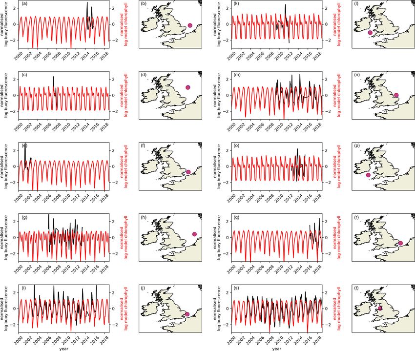
6178                                                                                          P. R. Halloran et al.: S2P3-R v2.0

downscale global models over small regions using complex               The biological model in S2P3 takes a lightweight and
3-D shelf sea models (e.g. Tinker and Howes, 2020) at con-          pragmatic view of representing primary production. Phyto-
siderable computational expense or downscale large-scale            plankton concentrations are modelled as a function of their
projections statistically (Van Hooidonk et al., 2016; e.g. Don-     initial concentration, vertical mixing, growth rate and a fixed
ner et al., 2005). Version 2 of the regional implementation of      grazing rate (Sharples, 2008). Phytoplankton growth rate is a
the Shelf Sea Physics and Primary Production (S2P3-R v2.0)          function of the maximum growth rate for a given temperature
aims to bridge the gap between high-complexity small-scale          and nutrient availability, modified by available photosynthet-
projections and large-scale statistical projections which ig-       ically active radiation (PAR) and maximum light utilisation
nore local processes and dynamics.                                  rate, minus respiration at a constant rate (Sharples, 2008).
   The underlying physical–biological model used in S2P3-           Surface PAR is set to 45 % of the net downwelling surface
R is the Shelf Sea Physics and Primary Production (S2P3)            shortwave radiation, and this decays as a function of phyto-
model (Simpson and Sharples, 2012). S2P3 makes the com-             plankton concentration and an attenuation coefficient which
mon assumption that in many regions variability on the shelf        is dependent on whether the water column is mixed or strat-
is dominated by atmospheric and tidal processes rather than         ified (Sharples, 2008). Nutrient availability is a function of
by communication with the open ocean (van der Molen et              vertical mixing, uptake by phytoplankton and loss through
al., 2017; e.g. Song et al., 2011), and consequently, repre-        grazing and is restored towards a constant concentration in
sents the ocean at a location as a 1-D column of water. The         the lowest model level (Sharples, 2008). The simple assump-
physical and biological components of S2P3 are discussed            tions made within the biological model align with the de-
below but are described in further detail in Simpson and            sire to keep the computational cost of the model low but also
Sharples (2012), Sharples et al. (2006), Sharples (2008) and        to avoid including poorly constrained processes within the
summarised in Marsh et al. (2015). S2P3-R v1.0 (Marsh et            model (Sharples, 2008). These simplifications and their im-
al., 2015) placed S2P3 into a spatial framework by repre-           pacts are discussed further in Sharples (2008). In its original
senting the shelf sea as a 2-D array of neighbouring indepen-       form, S2P3 was driven by sinusoidal time series of surface
dent 1-D columns of water. S2P3-R v2.0 addresses several            air temperature and pressure, relative humidity, total cloud
the limitations in S2P3-R v1.0, which prevented it from be-         cover and u and v surface winds.
ing used effectively to downscale large-scale reanalyses or
climate projections.
                                                                    3   Scientific advances from S2P3
2   Overview of the underlying 1-D model, S2P3                      Version 1 of S2P3-R modified the S2P3 code and provided
                                                                    bash scripts to run S2P3 as a 2-D array of 1-D column models
S2P3-R v2.0 is the second generation of regional-model
                                                                    to provide a computationally efficient way to simulate shelf
development building on the 1-D shelf sea model (S2P3)
                                                                    sea physical and biological conditions (Marsh et al., 2015).
(Sharples et al., 2006). The physical component of S2P3 sim-
                                                                    Application of this version of the model demonstrated that
ulates vertical profiles of temperature, turbulence and cur-
                                                                    this simple approach to shelf-sea modelling produced sen-
rents in response to tidal and wind driven mixing. The model
                                                                    sible patterns of temperature, stratification and primary pro-
calculates the tidal slope from the prescribed M2, S2, N2,
                                                                    duction on the Northwest European Shelf and East China and
O1 and K1 tidal ellipses, and from this, the water’s veloc-
                                                                    Yellow seas, and showed that the model reproduced observed
ity (Sharples et al., 2006). The stress applied by the tides is
                                                                    year-to-year variability at two sites in the English Channel
then calculated as a function of the velocity at 1m above the
                                                                    (Marsh et al., 2015). The success of S2P3-R at reproducing
seabed, the density of the seawater and a prescribed bottom
                                                                    physical and biological structures over the recent past has
drag coefficient (Sharples et al., 2006). The surface stress ex-
                                                                    motivated the developments and evaluation presented here.
erted by the wind is calculated as a function of wind speed
                                                                    The developments described here are aimed at running the
and direction (with respect to tides), air pressure and a wind-
                                                                    model at larger spatial scales and over longer time periods,
speed-dependent surface drag coefficient (Smith and Banke,
                                                                    including into the future to downscale and explore the coastal
1975). A turbulence closure scheme calculates profiles of
                                                                    implications of future climate change. These developments
vertical eddy viscosity and diffusivity as a function of current
                                                                    presented several practical challenges, which are discussed
shear and vertical density (Canuto et al., 2001). The surface
                                                                    below.
and bottom stress are propagated through the water column
                                                                       S2P3-R v1.0 introduced spatial information into its sim-
as a function of the vertical eddy viscosity, which is derived
                                                                    ulation by considering local bathymetry and tidal mixing,
from the turbulence closure scheme (Sharples et al., 2006).
                                                                    as well as a latitudinal dependence of the clear-sky radia-
S2P3 considers only the role of temperature, not salinity, on
                                                                    tion and Coriolis parameter used within the model (Marsh
density (Sharples et al., 2006), limiting its application in cold
                                                                    et al., 2015). Application of the model over larger spatial
water (where density variations are dominated by salinity), or
                                                                    domains was limited scientifically because it used common
variable salinity settings such as near river outflows.
                                                                    time series of surface air temperature and pressure, relative

Geosci. Model Dev., 14, 6177–6195, 2021                                             https://doi.org/10.5194/gmd-14-6177-2021
P. R. Halloran et al.: S2P3-R v2.0                                                                                              6179

humidity, cloud fraction and wind velocities to drive all wa-
ter columns within a simulation. S2P3-R v2.0 addresses this
limitation by utilising meteorological time series specific to
each grid location which are generated from reanalysis or
climate models using the provided scripts (see below and the
Code Availability section).
   Previous iterations of the model have represented down-
welling shortwave irradiance as a function of time of year,
latitude and total cloud fraction. While this approach has
been applied successfully when considering the Northwest
European Shelf (Sharples, 2008; Sharples et al., 2006; Marsh
et al., 2015), total cloud fraction cannot account for the im-
pacts on radiation of moving between regions of different
cloud type or changes in cloud microphysics. Over climate
timescales, changes in aerosol emissions, meteorology and
atmospheric chemistry will have considerable impacts on the
shortwave radiation received at the sea surface (Haywood
and Boucher, 2000), which may dominate greenhouse gas
driven climate signals at regional scales (Booth et al., 2012).
S2P3-R v2.0 moves to prescribing the net downwards sur-            Figure 1. Schematic description of the processes accounted for in
                                                                   S2P3-R v2.0 and prescribed quantities, both forcings and constants.
face radiation explicitly from the reanalysis product or cli-
                                                                   WOA stands for World Ocean Atlas.
mate model output from which it is driven.
   Analogous to the treatment of shortwave radiation within
S2P3, the net loss of heat from the surface of the ocean              To facilitate longer time steps in deeper waters, S2P3-R
in the form of longwave radiation was calculated in S2P3-          v1.0 scaled the vertical resolution in each water column with
R v1.0 from the temperature-dependent longwave emission            the water depth. This has been revised to a fixed 2 m verti-
derived from the Stefan–Boltzmann equation, moderated by           cal resolution in S2P3-R v2.0 to prevent variability in level
cloud fraction and humidity. This approach cannot account          thickness introducing spatial artefacts to simulated surface
for spatial/temporal changes in cloud-top height and opti-         water conditions. Phytoplankton growth in the model, and
cal thickness, which have been shown to be as important            therefore primary production, relies on a flux of nitrate into
as cloud fraction in determining the radiation field (Chen et      the lowest vertical level of the model. In S2P3-R v2.0, we
al., 2000). These factors are of first-order importance when       move from representing this as a single value in space and
relocating the model from high to low latitudes, perform-          time, to a value specific to each grid box, read in from an
ing simulations spanning these latitudes or considering the        ancillary file. A script is provided to generate this ancillary
impacts of anthropogenic aerosols and cloud feedbacks in           file from World Ocean Atlas (Levitus, 1982) data (see Code
response to climate change. A further limitation of infer-         Availability section).
ring the downwelling longwave radiation as a function of              A schematic overview of S2P3-R v2.0 is presented in
cloud fraction when performing long historical simulations         Fig. 1.
or simulations driven from future climate projections is that
the change in the radiation budget associated with changing
greenhouse gas concentrations is not directly accounted for.       4   Practical advances from S2P3
S2P3-R v2.0 revises the surface heat-loss through longwave
radiation (QLongwaveNet ) to                                       The practical developments made to version 2.0 of S2P3-R
                                                                   fall into two categories: (1) how the model runs and (2) how
QLongwaveNet = εlongwave σ T 4 − QLongwaveDownwards S,      (1)    to generate the data used to set up and force the model.
                                                                      The initial spatial implementation of S2P3 (S2P3-R v1.0)
where εlongwave is the longwave emissivity (0.985), σ is the       focused on what could be achieved by running S2P3 in
Stefan–Boltzmann constant (σ = 5.67 × 10⁻⁸ W m−2 K−4 ),            a regional sense and as such provided Bash scripts which
T is the temperature of the surface layer, QLongwaveDownwards      ran individual instances of the 1-D model for each of the
is the prescribed downwelling longwave radiation at the sur-       latitude–longitude locations specified in a domain file con-
face, and S is a constant to account for the fact that the model   taining depth and tidal forcing data. S2P3-R v2.0 makes sev-
is not simulating the ocean skin, where a proportion of the        eral changes to reduce the amount of input–output associated
longwave radiation will be absorbed and re-emitted without         with this approach and distributes the processing of water
interacting with the water at the depths represented by the top    columns over multiple processor cores. This is done by (1)
layer of the model.                                                re-writing the code which runs the underlying Fortran model

https://doi.org/10.5194/gmd-14-6177-2021                                              Geosci. Model Dev., 14, 6177–6195, 2021
6180                                                                                            P. R. Halloran et al.: S2P3-R v2.0

                                                                      5     Global evaluation

                                                                      S2P3-R v2.0 is an intentionally simple model. By ignoring
                                                                      lateral advection, one should expect to see model temper-
                                                                      ature biases in regions of heat convergence or divergence,
                                                                      i.e. where significant amounts of heat are imported or ex-
                                                                      ported through advection, or local dissipation rates are en-
                                                                      hanced through horizonal processes. The fact that a region
                                                                      may experience a temperature bias does not itself mean the
                                                                      model is not useful in that region. Despite biases in average
                                                                      temperatures, the model may still capture variability on the
                                                                      timescales of interest. The model variability may however
                                                                      be compromised if there is a temperature bias at low ambi-
                                                                      ent temperatures, where the non-linearity of the equation of
                                                                      state of seawater reduces the sensitivity of density to temper-
Figure 2. Processing time in hours to complete one year of simula-    ature variability. This limits the applicability of S2P3-R v2.0
tion at 0.2◦ resolution in a “global” (65◦ S–65◦ N, 180◦ W–180◦ E)    in cold waters, and alongside the specification of constant
configuration spanning water depths of 10–100 m. The high lati-       salinity and omission of sea ice processes, this means that
tudes were removed because the model assumes constant salinity        the evaluation of the model has been restricted to the subpo-
and the model does not include a representation of sea ice. Simula-   lar and lower-latitude ocean (
P. R. Halloran et al.: S2P3-R v2.0                                                                                                  6181

Figure 3. Overview of the S2P3-R v2.0 framework, which includes the model and runscript but also separate scripts to generate the required
input files. The arrows show where externally available data or the output from one component of S2P3-R V2.0 is supplied to another
component or output.

Table 1. Model inputs.

                    Model input                        Source                             Reference
                    Bathymetry global and              ETOPO1                             Amante and Eakins (2009)
                    NW European Shelf
                    Bathymetry Australia               3DGBR                              Beaman (2010)
                    Tides                              Produced using the Oregon          Egbert and Erofeeva (2002)
                                                       State University Tidal Inversion
                                                       Software (OTPS)
                    Meteorological forcing             ECMWF ERA5                         Hersbach et al. (2019)
                    Nutrients                          World Ocean Atlas 13               Levitus (1982)

typically corresponding to areas of weak tidal mixing, and             (Fig. 4). Conversely, the northern South China Sea and south-
a pervasive loss of stratification during the winter. If strong        ern Australia display low skill at capturing interannual vari-
tides played a first-order role in model skill, one would ex-          ability (Fig. 7), despite the model displaying low temperature
pect to see smaller model biases in the summer than winter             biases in these regions (Fig. 4). In the case of the South China
across the midlatitudes (Fig. 6); instead, we see little season-       Sea, this may relate to highly variable riverine freshwater in-
ality in the bias in much of the midlatitudes (e.g. Northwest          fluences on stratification.
European Shelf and Patagonian Shelf), stronger summer than
winter bias in the South China Sea and Bering Sea, and only            5.2    Global biogeochemical evaluation
smaller summer than winter biases in the Scotian and south-
ern Brazilian shelves.                                                 The biological component of S2P3 remains unchanged from
   Despite the model displaying average temperature biases             previous versions, apart from the addition of a spatially vary-
across some regions of up to ∼ 3 K, there is no consistent             ing nutrient field derived from the World Ocean Atlas (Levi-
relationship between such biases and the model’s ability to            tus, 1982) to which the bottom water nitrate is relaxed. S2P3
correctly simulate year-to-year variability (Fig. 7). More than        has previously been used to investigate biological questions
half of the year-to-year variability is captured by ∼ 60 % of          including investigating the drivers of timing of spring blooms
the simulated grid cells (Fig. 8). Squared Pearson’s prod-             in response to stratification (Sharples et al., 2006) and to ex-
uct moment correlations (R 2 ) calculated between (i) annual           plore the impact of tidal cycles on productivity (Sharples,
mean SST time series at each grid point from the ERA5                  2008) for typical Northwest European Shelf seas. More re-
forced S2P3R v2.0 simulations and (ii) satellite SST data              cently, a version of S2P3 has been developed to better rep-
(Merchant et al., 2019) from 2006–2016 (inclusive) demon-              resent the impacts of grazing and to include the impact of
strate high levels of skill in areas such as north of Australia,       photo-acclimation on phytoplankton growth (Bahamondes
the Java Sea and the Bering Sea (Fig. 7), despite these areas          Dominguez et al., 2020).
displaying significant positive or negative temperature biases

https://doi.org/10.5194/gmd-14-6177-2021                                                   Geosci. Model Dev., 14, 6177–6195, 2021
6182                                                                                                 P. R. Halloran et al.: S2P3-R v2.0

Figure 4. (a) Model SST simulation minus satellite SST data averaged between 1 January 2006 and 31 December 2016. White indicates that
the model is displaying no surface temperature bias, red indicates the model displays a warm bias, and blue indicates the model displays a
cool bias. The model was forced with atmospheric data from ERA5 (Hersbach et al., 2019). (b) Net surface downward heat flux calculated
from the ECMWF ERA5 reanalysis (Hersbach et al., 2019). Where this is positive, there is a net heat flux into the ocean. So, assuming that
system is approximately at steady state, heat is advected out of these areas. Where the net downward heat flux is negative there is advection
of heat into this region. S2P3-R V2.0 does not account for lateral advection, so one would anticipate that the model will display a warm bias
in regions where heat is typically advected from (i.e. tropics) and cool biases where heat is advected to (i.e. high latitudes).

                                                                            Evaluation of the model’s biological performance at a
                                                                         global scale is more challenging than the evaluation of sur-
                                                                         face temperature, because satellite chlorophyll-a products
                                                                         are often unreliable in shallow waters, where suspended sed-
                                                                         iment, coloured dissolved organic matter (CDOM) and bot-
                                                                         tom reflection influence the retrievals considerably (Darecki
                                                                         and Stramski, 2004). The analysis presented here uses the
                                                                         European Space Agency Climate Change Initiative (ESA
                                                                         CCI) chlorophyll-a product data (Sathyendranath et al.,
                                                                         2020) but filters out waters shallower than 70 m (Sathyen-
                                                                         dranath et al., 2019) to avoid the issues mentioned above.
                                                                         The model demonstrates low (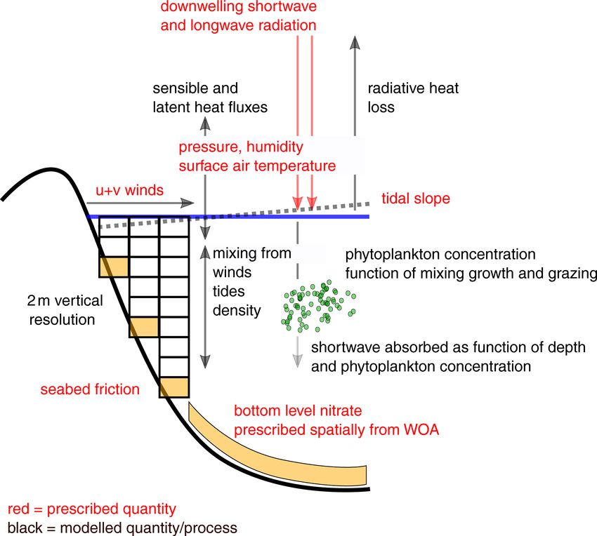
P. R. Halloran et al.: S2P3-R v2.0                                                                                                 6183

Figure 6. Annual mean SST bias (a) and difference in absolute SST bias between summer and winter (b). In panel (b), blue indicates that
the summer months (June, July, August in the Northern Hemisphere; December, January, February in the Southern Hemisphere) display a
smaller absolute bias than the winter months (December, January, February in the Northern Hemisphere; June, July, August in the Southern
Hemisphere).

Figure 7. Pearson’s R 2 calculated between annual mean model SST
simulation and annual mean satellite SST data (Merchant et al.,
2019) between 2006 and 2016.
                                                                      Figure 8. Sorted R and R 2 values from all grid cells calculated
                                                                      from global shelf-sea SST simulation correlation with satellite SST
Overestimation of chlorophyll-a may therefore be a response           (Fig. 7).
to positive seawater temperature biases, or both may be re-
sponding to a positive shortwave radiation bias.
   To facilitate a more detailed understanding of the model           framework appear to work well (Fig. 4), and it is a large area
performance, we now evaluate the model in one midlati-                of shallow water which has previously been studied in de-
tude region, the Northwest European Shelf, then one lower-            tail both observationally (e.g. Smyth et al., 2015) and using
latitude region, the Great Barrier Reef.                              state-of-the-art 3-D models (e.g. Graham et al., 2018).
                                                                         Forced with the ERA5 atmospheric data (Hersbach et
                                                                      al., 2019), S2P3-R v2.0 simulates the time-averaged SST
6   Northwest European Shelf physical evaluation                      within 0.5 K across much of the Northwest European Shelf
                                                                      (Fig. 10). The model also simulates the trend and interan-
The Northwest European Shelf is both typical of the midlat-           nual variability in SST well in the North Sea, English Chan-
itude regions, where the assumptions made in this modelling           nel and Irish Sea (Fig. 11), despite the North Sea and En-

https://doi.org/10.5194/gmd-14-6177-2021                                                 Geosci. Model Dev., 14, 6177–6195, 2021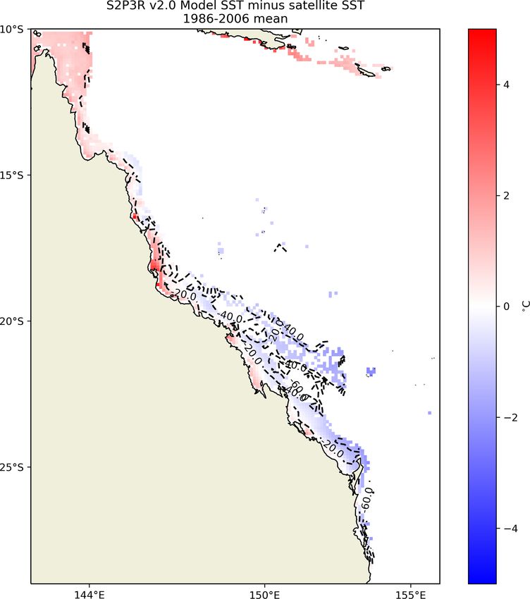
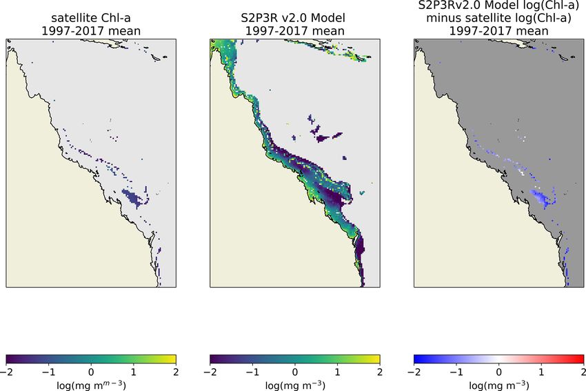
6184                                                                                                 P. R. Halloran et al.: S2P3-R v2.0

Figure 9. Comparison of surface level chlorophyll-a concentrations with satellite based chlorophyll-a estimates (Sathyendranath et al.,
2020). Figures present an annual mean of all data available between 1997 and 2017 inclusive. Satellite data are filtered to include minimised
issues associated with case-2 waters by selecting water ≥ 70 m water depth. The nutrient data to which the water in the model’s bottom level
was relaxed to are taken from the winter values in World Ocean Atlas for each hemisphere.

Geosci. Model Dev., 14, 6177–6195, 2021                                                    https://doi.org/10.5194/gmd-14-6177-2021
P. R. Halloran et al.: S2P3-R v2.0                                                                                            6185

                                                                    Northwest European Shelf biogeochemical evaluation

                                                                    S2P3R v2.0 underestimates surface chlorophyll-a when
                                                                    compared to annual mean satellite derived estimates
                                                                    (Sathyendranath et al., 2020) across most of the Northwest
                                                                    European Shelf by 0.25 to 0.50 mg m−3 (Fig. 13). The small-
                                                                    est bias is seen in the North Sea and the largest in the Irish
                                                                    Sea (Fig. 13).
                                                                       The seasonal and interannual variability of phytoplank-
                                                                    ton production, and therefore chlorophyll-a concentration
                                                                    are strongly influenced by changes in stratification. Where
                                                                    the water column is mixed throughout the year (e.g. English
                                                                    channel and southern North Sea), phytoplankton growth
                                                                    tends to display a single peak governed to a first order by
                                                                    the cycle of solar irradiance and the availability of nutrients,
                                                                    with development of the peak slowed by mixing of phyto-
                                                                    plankton into deeper, poorly lit, waters (e.g. Fig. 14a, c, e,
                                                                    g, i, j) (Wafar et al., 1983). Where the water column is sea-
                                                                    sonally stratified and winter mixing has removed any upper-
                                                                    water column nutrient limitation potential, a spring bloom
Figure 10. S2P3R v2.0 SST averaged between the years 1986           typically develops as the mixed layer – defined by turbu-
and 2006 inclusive minus satellite SSTs (Merchant et al., 2019)     lence levels (Chiswell, 2011; Chiswell et al., 2015) – shal-
averaged over the same interval. Labelled dashed lines illustrate   lows across a seasonally deepening critical depth, shallower
bathymetry in metres.                                               than which light-limited phytoplankton production exceeds
                                                                    approximately depth-invariant phytoplankton losses (Sver-
                                                                    drup, 1953). In these seasonally stratified waters, an autumn
glish Channel displaying cool and warm temperature biases           bloom (and therefore second chlorophyll-a peak) may also
of approximately 0.5 K respectively (Fig. 11). The cool bias        develop as cooling results in buoyancy loss from the surface
in the northern North Sea is consistent with the model not ac-      or winds increase turbulence, and the mixed layer deepens
counting for the inflow of relatively warm Atlantic Water via       and refreshes what have become nutrient-limited sunlit wa-
the Dooley Current between Orkney and Shetland (Dooley,             ters, with nutrients from deeper in the water column (Findlay
1974; Marsh et al., 2017; Sheehan et al., 2020).                    et al., 2006). This potentially skewed, bimodal distribution is
   Bottom water temperatures can be examined at individual          captured by the model in seasonally stratified sites (Fig. 14c,
locations using mooring data, as done in Marsh et al. (2015),       k, o). While in the central North Sea and Celtic Sea, the sea-
or at sparse locations against gridded data (e.g. Good et           sonal evolution of model chlorophyll-a concentrations match
al., 2013), but to facilitate a more spatially complete assess-     closely with that inferred from observations (Fig. 14c, k, o),
ment we here turn to state-of-the-art model output, generated       at most sites the model fails to capture the full complexity of
by the 1.5 km Nucleus for European Modelling of the Ocean           the seasonal signal. The model also fails to capture the inter-
(NEMO) shelf Atlantic Margin Model (AMM15) (Graham                  annual variability in chlorophyll-a at those sites where long-
et al., 2018). We find that S2P3-R v2.0 replicates the average      enough observational time series exist to assess this (Fig. 14).
values and interannual variability in bottom water tempera-         The lack of evidence for correctly simulated interannual vari-
tures in the North Sea, English Channel and Irish Sea cap-          ability potentially reflects the importance of processes not
tured by the AMM15 model (Graham et al., 2018) with bi-             represented in this model such as photo-acclimation (Ba-
ases of less than 0.5 K and R 2 values of 0.92, 0.84 and 0.93       hamondes Dominguez et al., 2020), grazing (Bahamondes
the North Sea, English Channel and Irish Sea, respectively          Dominguez et al., 2020) and phytoplankton species composi-
(Fig. 12). While the AMM15 model is not a perfect surro-            tion (Barnes et al., 2015) in controlling interannual variabil-
gate for observations, this comparison gives us confidence          ity or the importance of variability in nutrient flux across the
in these regions that the use of the highly computationally         shelf break (Holt et al., 2012) and from rivers (Capuzzo et
efficient S2P3-R v2.0 model to a first order gives us com-          al., 2018).
parable bottom water temperature results to a state-of-the-
art and computationally demanding three-dimensional mod-
elling system.                                                      7   Great Barrier Reef physical evaluation

                                                                    Moving to the low latitudes where SST biases in the S2P3R
                                                                    v2.0 model are typically larger than they are in the midlat-

https://doi.org/10.5194/gmd-14-6177-2021                                              Geosci. Model Dev., 14, 6177–6195, 2021
6186                                                                                             P. R. Halloran et al.: S2P3-R v2.0

Figure 11. S2P3R v2.0 SST averaged annually and across the three regions highlighted in inset maps and annually averaged satellite SSTs
(Merchant et al., 2019) from the same regions.

Figure 12. S2P3R v2.0 bottom water temperatures averaged annually and across the three regions highlighted in inset maps and annually
bottom water temperatures from these same regions taken from a state-of-the art shelf sea model hindcast (Graham et al., 2018).

Geosci. Model Dev., 14, 6177–6195, 2021                                                https://doi.org/10.5194/gmd-14-6177-2021
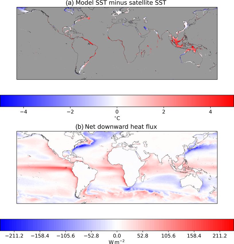
P. R. Halloran et al.: S2P3-R v2.0                                                                                                   6187

Figure 13. Comparison of Northwest European Shelf surface level chlorophyll-a concentrations with satellite based chlorophyll-a estimates
(Sathyendranath et al., 2020). Figures present an annual mean of all data available between 1997 and 2017 inclusive. Dashed lines represent
20 m depth contours. Satellite data are filtered to minimise the influence of case-2 waters by focusing on water ≥ 70 m water depth.

Figure 14. Comparison of model chlorophyll-a time series (red) with chlorophyll-a fluorescence measurements (black) made on 10 au-
tonomous buoys situated round the UK as part of the Cefas SmartBuoy network (Sivyer, 2016). Both datasets have been averaged monthly
and logged, had the time series mean removed and have been normalised by their standard deviation. Fluorescence data have been filtered to
include only that collected between 18:00 and 06:00 LT to avoid quenching of the signal by sunlight. Maps on the right-hand side illustrate
the location of each buoy. Note that buoys have been operational over different time windows.

https://doi.org/10.5194/gmd-14-6177-2021                                                   Geosci. Model Dev., 14, 6177–6195, 2021
6188                                                                                           P. R. Halloran et al.: S2P3-R v2.0

                                                                     mated Intelligent Monitoring of Marine Systems) sensor
                                                                     network. The following IMOS FAIMMS sites have been
                                                                     use: Heron Island South Shelf (GBRHIS, Integrated Marine
                                                                     Observing System, 2009a); Lizard Island Shelf (GBRLSH,
                                                                     Integrated Marine Observing System, 2009b); Palm Pas-
                                                                     sage Shelf (GBRPPS, Integrated Marine Observing System,
                                                                     2009d), Yongala mooring (NRSYON, Australian Institute
                                                                     of Marine Science, 2020); One Tree Island Shelf mooring
                                                                     (GBROTE, Integrated Marine Observing System, 2009c) and
                                                                     the Ningaloo mooring (NRSNIN, Integrated Marine Observ-
                                                                     ing System, 2017). The locations of the moorings utilised in
                                                                     the evaluation presented here are highlighted in Fig. 17.
                                                                        In situ observations indicate that a cool bias exists in the
                                                                     modelled SSTs, but this is restricted to austral winter months
                                                                     (Fig. 17c). The fact that a warm bias is not evident in the
                                                                     mooring data, as it is in the satellite SST data (Fig. 15), may
                                                                     result from a sampling bias within the mooring dataset to-
                                                                     wards deeper waters. Modelled bottom water temperatures
                                                                     from the lower-latitude mooring sites present a cool bias, but
                                                                     a linear relationship when compared with observational data
                                                                     (Fig. 17d). The cool bias may reflect the fact that the model
                                                                     output against which the observations are compared repre-
                                                                     sent a mean value across a ∼ 10 km2 grid cell and, for exam-
Figure 15. S2P3R v2.0 SST averaged between 1986 and 2006 in-         ple, may well therefore not be simulating the conditions at
clusive minus satellite SSTs (Merchant et al., 2019) over the same   the same depth as the observations are made.
interval. Labelled dashed lines show bathymetry in metres.
                                                                     Great Barrier Reef biogeochemical evaluation

itudes (Fig. 4), a simulation has been undertaken which en-          A comparison is made between the S2P3R v2.0 simulation of
compasses the Great Barrier Reef (GBR). The GBR is well              chlorophyll and annually averaged ESA CCI long-term satel-
instrumented, allowing analysis of subsurface as well as sur-        lite chlorophyll data (Sathyendranath et al., 2020). The ESA
face temperatures in this region.                                    CCI long-term satellite chlorophyll product is focused on
   The modelled SSTs in the GBR display a positive bias rel-         case-1 waters (Sathyendranath et al., 2019). The comparison
ative to satellite SSTs in the north and negative bias in the        presented here is therefore restricted to water depths ≥ 70 m,
south (Fig. 15). This may relate to the fact that the model          a compromise which allows us to exclude the most coastally
does not simulate lateral advection, which will be exporting         influenced waters while maintaining moderate spatial cov-
heat from the north to the south in the East Australian Cur-         erage. The S2P3R v2.0 simulation of chlorophyll displays
rent.                                                                low negative biases
P. R. Halloran et al.: S2P3-R v2.0 6189
Figure 16. Comparison of interannual SST variability between S2P3R v2.0 and satellite (Merchant et al., 2019) over the GBR, subdivided
into three latitudinally delineated regions. These regions are identified in the inset maps.
drup, 1953) with the seabed at these high-light and shallow exchanges with the deep ocean or runoff. When compared
locations. The incomplete or short lengths of the GBR flu- to satellite data (Merchant et al., 2019), 61 % of grid cells
orescence observational datasets mean that it is not possible however present an SST bias of greater than 1 K and 42 %
to undertake a detailed investigation of interannual variabil- present an SST bias of greater than 2 K, highlighting limita-
ity; however, the longest of the mooring datasets (Fig. 19k) tions to the simple modelling approach.
exhibits its lowest chlorophyll-a peaks in the same years as Together, analysis of SST variability and SST bias indi-
those simulated by the model (2018 and 2019). In a typically cates that there are significant areas of our global shelf seas
oligotrophic setting, like much of the GBR, one might expect where the model should be used with extreme caution. These
year-to-year variability to be dominated by injections of nu- regions are likely to be those which have (1) substantial ex-
trients from the shelf break or the coast (Furnas and Mitchell, change of heat with the open ocean through lateral advec-
1986). Despite the model not representing these processes, tion, (2) low tidally driven mixing and therefore a low ratio
it nevertheless simulates considerable interannual variability, of vertical/horizontal control over SSTs (Fig. 5), (3) signifi-
indicating the potential for atmospheric and vertical ocean cant influences from local processes/properties such as river-
dynamics drivers of such variability. ine inputs or locally unusual bottom drag coefficients, (4)
high salinity variability and low temperatures, or (5) on-shelf
propagation and dissipation of the internal tide. The model
8 Summary and discussion could however be tuned to account for some of these influ-
ences if studies were to be undertaken with a focus on such
Forced by observation-derived atmospheric conditions, a regions.
simulation spanning the shelf seas of the global tropical-to- Regional evaluation has been conducted across the North-
subpolar ocean at approximately 10 km2 resolution captures west European Shelf around the UK and the Great Barrier
>50 % of the observed interannual SST variability between Reef. The model captures most of the observed SST trend
2006 and 2016 in ∼ 60 % of the grid cells, and greater than and variability in the waters around the UK (Fig. 11), with
80 % of the interannual SST variability in ∼ 20 % of the grid a temperature biases of6190 P. R. Halloran et al.: S2P3-R v2.0 Figure 17. Comparison of S2P3R v2.0 surface (a, b) and bottom (c, d) temperatures against mooring observations from IMOS and FAIMMS and moorings (Integrated Marine Observing System; IMOS). Facility for the Automated Intelligent Monitoring of Marine Systems – FAIMMS; GBRHIS: Heron Island South Shelf mooring component of the GBR mooring array; GBRLSH: Lizard Island Shelf mooring component of the GBR mooring array; GBRPPS: Palm Passage Shelf mooring component of the GBR mooring array; Northern Australia Automated Marine Weather and Oceanographic Stations, sites: Yongala mooring (NRSYON); GBROTE: One Tree Island Shelf mooring component of the GBR mooring array; IMOS – ANMN National Reference Station (NRS) Ningaloo mooring (NRSNIN). The x − y values of the data presented in plots on the top and bottom (a and b, and c and d) are identical but are coloured to highlight where temporal and geographical biases exist in the model output. Seabed observations are considered here to be those falling within 5 m of the site depth for each mooring. The map shows the location of surface (red) and bottom (blue) temperature mooring observations used in model evaluation over the GBR. Figure 18. Comparison of GBR surface level chlorophyll-a concentrations with satellite based chlorophyll-a estimates (Sathyendranath et al., 2020). Figures present an annual mean of all data available between 1997 and 2017 inclusive. Satellite data are filtered to include just water ≥ 70 m to minimise contamination by case-2 waters. Geosci. Model Dev., 14, 6177–6195, 2021 https://doi.org/10.5194/gmd-14-6177-2021
P. R. Halloran et al.: S2P3-R v2.0                                                                                                 6191

                                                                            A particular strength of this modelling approach is likely
                                                                         to be in examining or predicting anomalies or extremes
                                                                         which occur under a consistent set of oceanographic condi-
                                                                         tions. For example, the marine heat waves associated with
                                                                         tropical coral bleaching tend to occur following doldrum-
                                                                         like condition, when there is limited advection and mixing
                                                                         (Skirving et al., 2011).
                                                                            Observational limitations mean the model’s simulation of
                                                                         biological production in space and time is harder to assess
                                                                         than that of temperature. The model however captures the
                                                                         broad-scale patterns of surface chlorophyll (Figs. 9, 13, 18),
                                                                         with a weak indication of latitudinally varying bias towards
                                                                         overprediction in low latitudes and underprediction in high
                                                                         latitudes (Fig. 9). While the model displays considerable skill
                                                                         in many locations at simulating intra-annual chlorophyll vari-
                                                                         ability (Figs. 14, 19), it demonstrates no skill at simulat-
                                                                         ing interannual chlorophyll variability. This implies that the
                                                                         large-scale processes which govern the seasonal progression
                                                                         of primary production do not also govern interannual vari-
                                                                         ability. Factors such as riverine input of nutrients may dom-
                                                                         inate interannual variability in many locations (Lenhart et
                                                                         al., 1997). These results emphasise the importance of decadal
                                                                         and longer observational biogeochemical time series for as-
                                                                         sessing the skill of models at simulating those processes
                                                                         which are likely to govern the biogeochemical response of
                                                                         our shelf seas to anthropogenic climate change.
                                                                            In summary, S2P3R v2.0 is a simple-to-use, computa-
                                                                         tionally efficient shelf sea modelling tool ideally suited to
                                                                         (a) semi-dynamically downscale climate projections, (b) un-
                                                                         dertake large-scale, long or large-ensemble projections, (c)
                                                                         use after careful evaluation by management or policy groups
Figure 19. Comparison of model chlorophyll-a time series (red)
                                                                         without access to large technical or computational resources.
with chlorophyll-a fluorescence measurements (black) made on
six moored buoys situated down the GBR as part of the IMOS
                                                                         The objective assessment of the model presented here will
FAIMMS. Both datasets have been averaged monthly and logged,             hopefully guide potential users as to whether S2P3R v2.0 is
had the time series mean removed and have been normalised by             the tool to answer their questions. Where S2P3R v2.0 is con-
their standard deviation. Surface level data were not available for      sidered to be an appropriate tool, we would encourage local
all sites, so data represent an average over the top 12 m of the water   assessment of the data presented here at a global scale and
column to improve spatial data coverage.                                 hope to facilitate this through the provision of these data (see
                                                                         Data Availability section). Finally, within the Code Availabil-
                                                                         ity section of this paper, we provide the model code, code re-
a state-of-the-art shelf sea model hindcast (Graham et al.,              quired to produce the model forcing datasets, and an example
2018) for the three focal regions of the North Sea, English              model setup with pre-prepared forcing data, and within the
Channel and Irish Sea. Comparison of modelled and satel-                 readme file, we provide step-by-step instructions for setting
lite SSTs across the Great Barrier Reef indicates that over              up and running the model.
∼ 10-year intervals the model performs well, but there ap-
pear to be step changes in the modelled SST which are not
seen in the satellite data. The discontinuity occurring around           Code availability. S2P3Rv2.0 is available on GitHub: https:
the year 2000 may reflect a step change in the data assimila-            //github.com/PaulHalloran/S2P3Rv2.0 (last access: 21 Septem-
tion configuration used within the ERA5 product or data be-              ber 2021).
ing assimilated by that product (Hersbach et al., 2018) used                The release associated with this paper (https://github.com/
to provide the atmospheric forcing to S2P3R v2.0. Alterna-               PaulHalloran/S2P3Rv2.0/releases/tag/v1.0.1,      last   access:
tively, the step changes may result from changes in the lateral          21 September 2021) has been archived on Zenodo with the
supply of heat from the open ocean.                                      following DOI: https://doi.org/10.5281/zenodo.4147559 (Halloran,
                                                                         2020a).

https://doi.org/10.5194/gmd-14-6177-2021                                                   Geosci. Model Dev., 14, 6177–6195, 2021
6192 P. R. Halloran et al.: S2P3-R v2.0
The readme file available on GitHub or via the DOI link provides versity of Exeter and University of Queensland Partnership. This
step-by-step instructions for how to install, set up and run the model, project has received funding from the European Union’s Hori-
and it provides a basic script for analysing the model output. At the zon 2020 research and innovation programme under grant agree-
bottom of the readme, a worked example is provided to help the ment no. 820989 (project COMFORT, Our common future ocean in
user go through the full process from generating model forcing files, the Earth system – quantifying coupled cycles of carbon, oxygen,
running the model and displaying the output with some example and nutrients for determining and achieving safe operating spaces
data. with respect to tipping points). William Skirving received fund-
ing by NOAA (grant no. NA19NES4320002) (Cooperative Insti-
tute for Satellite Earth System Studies) at the University of Mary-
Data availability. The model minus satellite SST data from the land/ESSIC.
global (65◦ S–65◦ N) simulation averaged between 2006 and 2016,
from which the global validation has been undertaken in this pa-
per, is archived as NetCDF and csv files to allow potential users to Review statement. This paper was edited by Simone Marras and re-
undertake bespoke assessment of the model http://doi.org/10.5281/ viewed by two anonymous referees.
zenodo.4018815 (Halloran, 2020b).
Author contributions. The model development was undertaken by
References
PRH. PRH lead the analysis with contributions from JKMW,
BAN, RM and WS. All authors contributed to the writing of the
Amante, C. and Eakins, B. W.: ETOPO1 1 Arc-Minute
manuscript.
Global Relief Model: Procedures, Data Sources and
Analysis, NOAA Tech. Memo., NESDIS NGDC-24,
https://doi.org/10.1594/PANGAEA.769615, 2009.
Competing interests. The authors declare that they have no conflict Australian Institute of Marine Science (AIMS):
of interest. NRSYON: Northern Australia Automated Marine
Weather and Oceanographic Stations, Sites: [Yongala],
https://doi.org/10.25845/5c09bf93f315d, 2020.
Disclaimer. This paper reflects only the authors’ views; the Euro- Bahamondes Dominguez, A. A., Hickman, A. E., Marsh, R.,
pean Commission and their executive agency are not responsible and Moore, C. M.: Constraining the response of phytoplank-
for any use that may be made of the information the work contains. ton to zooplankton grazing and photo-acclimation in a temper-
William Skirving was supported by NOAA at the University ate shelf sea with a 1-D model – towards S2P3 v8.0, Geosci.
of Maryland/ESSIC. The scientific results and conclusions, as Model Dev., 13, 4019–4040, https://doi.org/10.5194/gmd-13-
well as any views or opinions expressed herein, are those of the 4019-2020, 2020.
author(s) and do not necessarily reflect the views of NOAA or the Barnes, M. K., Tilstone, G. H., Suggett, D. J., Widdicombe,
Department of Commerce. C. E., Bruun, J., Martinez-Vicente, V., and Smyth, T. J.:
Temporal variability in total, micro- and nano-phytoplankton
Publisher’s note: Copernicus Publications remains neutral with primary production at a coastal site in the Western En-
regard to jurisdictional claims in published maps and institutional glish Channel, Prog. Oceanogr., 137 (Part B), 470–483,
affiliations. https://doi.org/10.1016/j.pocean.2015.04.017, 2015.
Beaman, R.: Project 3DGBR: a high-resolution depth model
for the Great Barrier Reef and Coral Sea, MTSRF Final
Acknowledgements. The SmartBuoy data were made available by Report Project 2.5i.1a, Reef and Rainforest Research Cen-
Cefas and funded by Defra and the UK Research Council Can- tre MTSRF Final Report Marine and Tropical Sciences
dyfloss and Celtic Deep2 (grant no. NE/K001957/1). The IMOS Research Facility, James Cook University, available at:
buoy data were provided by the IMOS Queensland and Northern https://www.deepreef.org/images/stories/publications/reports/
Australian Moorings subfacility of the Australian National Mooring Project3DGBRFinal_RRRC2010.pdf (last access: 1 July 2021),
Network funded by the Australian Institute of Marine Science and 2010.
the Integrated Marine Observing System (IMOS) is enabled by the Booth, B. B. B., Dunstone, N. J., Halloran, P. R., Andrews, T., and
National Collaborative Research Infrastructure Strategy (NCRIS), Bellouin, N.: Erratum: Aerosols implicated as a prime driver of
supported by the Australian Government. It is operated by a con- twentieth-century North Atlantic climate variability, Nature, 484,
sortium of institutions as an unincorporated joint venture, with the 228–232, https://doi.org/10.1038/nature11138, 2012.
University of Tasmania as lead agent (https://www.imos.org.au, last Bowen, B. W., Gaither, M. R., DiBattista, J. D., Iac-
access: 1 July 2021). chei, M., Andrews, K. R., Grant, W. S., Toonen, R. J.,
and Briggs, J. C.: Comparative phylogeography of the
ocean planet, P. Natl. Acad. Sci. USA, 113, 7962–7969,
Financial support. Paul Halloran received funding by the UK Re- https://doi.org/10.1073/pnas.1602404113, 2016.
search Council (grant no. NE/V00865X/1). Paul Halloran and Jen- Canuto, V. M., Howard, A., Cheng, Y., and Dubovikov,
nifer McWhorter received funding by the QUEX Institute, a Uni- M. S.: Ocean turbulence. Part I: One-point closure
model-momentum and heat vertical diffusivities, J. Phys.
Geosci. Model Dev., 14, 6177–6195, 2021 https://doi.org/10.5194/gmd-14-6177-2021P. R. Halloran et al.: S2P3-R v2.0 6193 Oceanogr., 31, 1413–1426, https://doi.org/10.1175/1520- to global scales SUBMISSION (v1.0.1), Zenodo [code], 0485(2001)0312.0.CO;2, 2001. https://doi.org/10.5281/zenodo.4147559, 2020a. Capuzzo, E., Lynam, C. P., Barry, J., Stephens, D., Forster, R. M., Halloran, P.: S2P3Rv2.0 bias data, Zenodo [data set], Greenwood, N., McQuatters-Gollop, A., Silva, T., van Leeuwen, https://doi.org/10.5281/zenodo.4018815, 2020b. S. M., and Engelhard, G. H.: A decline in primary production Haywood, J. and Boucher, O.: Estimates of the direct and indirect in the North Sea over 25 years, associated with reductions in radiative forcing due to tropospheric aerosols: A review, Rev. zooplankton abundance and fish stock recruitment, Glob. Chang. Geophys., 38, 513–543, https://doi.org/10.1029/1999RG000078, Biol., 24, e352–e364, https://doi.org/10.1111/gcb.13916, 2018. 2000. Chen, T., Rossow, W. B., and Zhang, Y.: Ra- Hersbach, H., De Rosnay, P., Bell, B., Schepers, D., Simmons, A., diative effects of cloud-type variations, J. Cli- Soci, C., Abdalla, S., Balmaseda, A., Balsamo, G., Bechtold, mate, 13, 264–286, https://doi.org/10.1175/1520- P., Berrisford, P., Bidlot, J., De Boisséson, E., Bonavita, M., 0442(2000)0132.0.CO;2, 2000. Browne, P., Buizza, R., Dahlgren, P., Dee, D., Dragani, R., Dia- Chiswell, S. M.: Annual cycles and spring blooms in phytoplank- mantakis, M., Flemming, J., Forbes, R., Geer, A., Haiden, T., ton: Don’t abandon Sverdrup completely, Mar. Ecol. Prog. Ser., Hólm, E., Haimberger, L., Hogan, R., Horányi, A., Janisková, 443, 39–50, https://doi.org/10.3354/meps09453, 2011. M., Laloyaux, P., Lopez, P., Muñoz-Sabater, J., Peubey, C., Radu, Chiswell, S. M., Calil, P. H. R., and Boyd, P. W.: Spring blooms and R., Richardson, D., Thépaut, J.-N., Vitart, F., Yang, X., Zsótér, annual cycles of phytoplankton: A unified perspective, J. Plank- E., and Zuo, H.: Operational global reanalysis: progress, future ton Res., 37, 500–508, https://doi.org/10.1093/plankt/fbv021, directions and synergies with NWP including updates on the 2015. ERA5 production status, ERA Rep. Ser., Document Number 27, Darecki, M. and Stramski, D.: An evaluation of MODIS and SeaW- https://doi.org/10.21957/tkic6g3wm, 2018. iFS bio-optical algorithms in the Baltic Sea, Remote Sens. En- Hersbach, H., Bell, B., Berrisford, P., Horányi, A., Sabater, J. M., viron., 89, 326–350, https://doi.org/10.1016/j.rse.2003.10.012, Nicolas, J., Radu, R., Schepers, D., Simmons, A., Soci, C., 2004. Doney, S. C.: The Growing Human Footprint on Coastal and Dee, D.: Global reanalysis: goodbye ERA-Interim, hello and Open-Ocean Biogeochemistry, Science, 328, 1512–1516, ERA5, ECMWF Newsl., Newsletter number 159, pp. 17–24, https://doi.org/10.1126/science.1185198, 2010. https://doi.org/10.21957/vf291hehd7, 2019. Donner, S. D., Skirving, W. J., Little, C. M., Oppenheimer, M., Holt, J., Harle, J., Proctor, R., Michel, S., Ashworth, M., Batstone, and Hoegh-Gulberg, O.: Global assessment of coral bleaching C., Allen, I., Holmes, R., Smyth, T., Haines, K., Bretherton, D., and required rates of adaptation under climate change, Glob. and Smith, G.: Modelling the global coastal ocean, Philos. Trans. Chang. Biol., 11, 2251–2265, https://doi.org/10.1111/j.1365- R. Soc. A, 367, 939–951, https://doi.org/10.1098/rsta.2008.0210, 2486.2005.01073.x, 2005. 2009. Dooley, H. D.: Hypotheses concerning the circulation of Holt, J., Butenschön, M., Wakelin, S. L., Artioli, Y., and Allen, J. I.: the northern North Sea, ICES J. Mar. Sci., 36, 54–61, Oceanic controls on the primary production of the northwest Eu- https://doi.org/10.1093/icesjms/36.1.54, 1974. ropean continental shelf: model experiments under recent past Egbert, G. D. and Erofeeva, S. Y.: Efficient inverse mod- conditions and a potential future scenario, Biogeosciences, 9, eling of barotropic ocean tides, J. Atmos. Ocean. 97–117, https://doi.org/10.5194/bg-9-97-2012, 2012. Technol., 19, 183–204, https://doi.org/10.1175/1520- Integrated Marine Observing System (IMOS): GBRHIS: Heron 0426(2002)0192.0.CO;2, 2002. Island South Shelf Mooring component of the GBR Moor- Findlay, H. S., Yool, A., Nodale, M., and Pitchford, J. W.: Modelling ing Array, available at: https://apps.aims.gov.au/metadata/ of autumn plankton bloom dynamics, J. Plankton Res., 28, 209– view/9a19eaa5-6069-4ed6-b004-5f7590664881, (last access: 220, https://doi.org/10.1093/plankt/fbi114, 2006. 21 September 2021), 2009a. Furnas, M. J. and Mitchell, A. W.: Phytoplankton dynamics in Integrated Marine Observing System (IMOS): GBRLSH: the central Great Barrier Reef-I. Seasonal changes in biomass Lizard Island Shelf Mooring component of the GBR Moor- and community structure and their relation to intrusive activ- ing Array, available at: https://apps.aims.gov.au/metadata/ ity, Cont. Shelf Res., 6, 363–384, https://doi.org/10.1016/0278- view/ee39900f-141e-43a6-8261-0164267c8f95 (last access: 4343(86)90078-6, 1986. 21 September 2021), 2009b. Good, S. A., Martin, M. J., and Rayner, N. A.: EN4: Integrated Marine Observing System (IMOS): GBROTE: One Quality controlled ocean temperature and salinity pro- Tree Island Shelf Mooring component of the GBR Moor- files and monthly objective analyses with uncertainty ing Array, available at: https://apps.aims.gov.au/metadata/ estimates, J. Geophys. Res. Ocean., 118, 6704–6716, view/05c9319d-ebde-4ba5-8c25-08ea82cbe77f (last access: https://doi.org/10.1002/2013JC009067, 2013. 21 September 2021), 2009c. Graham, J. A., O’Dea, E., Holt, J., Polton, J., Hewitt, H. T., Furner, Integrated Marine Observing System (IMOS): GBRPPS: Palm R., Guihou, K., Brereton, A., Arnold, A., Wakelin, S., Castillo Passage Shelf Mooring component of the GBR Moor- Sanchez, J. M., and Mayorga Adame, C. G.: AMM15: a new ing Array, available at: https://apps.aims.gov.au/metadata/ high-resolution NEMO configuration for operational simulation view/11c307bd-89bf-4616-b3df-52645ca56b6e (last access: of the European north-west shelf, Geosci. Model Dev., 11, 681– 21 September 2021), 2009d. 696, https://doi.org/10.5194/gmd-11-681-2018, 2018. Integrated Marine Observing System (IMOS): IMOS – ANMN Halloran, P.: PaulHalloran/S2P3Rv2.0: S2P3-R v2.0: compu- National Reference Station (NRS) Ningaloo Mooring tationally efficient modelling of shelf seas on regional (NRSNIN), available at: https://apps.aims.gov.au/metadata/ https://doi.org/10.5194/gmd-14-6177-2021 Geosci. Model Dev., 14, 6177–6195, 2021
6194                                                                                                    P. R. Halloran et al.: S2P3-R v2.0

   view/a581c961-8632-497f-bc5e-2002957577ec (last access:                    Steinmetz, F., Steele, C., Swinton, J., Valente, A., Zühlke, M.,
   21 September 2021), 2017.                                                  Feldman, G., Franz, B., Frouin, R., Werdell, J., and Platt, T.: ESA
Integrated Marine Observing System (IMOS): Facility for                       Ocean Colour Climate Change Initiative (Ocean_Colour_cci):
   the Automated Intelligent Monitoring of Marine Systems                     Global chlorophyll-a data products gridded on a sinusoidal pro-
   – FAIMMS, available at: https://apps.aims.gov.au/metadata/                 jection, Version 4.2, Cent. Environ. Data Anal., Centre for En-
   view/d63dc150-0d02-11dd-bbbb-00008a07204e, last access:                    vironmental Data Analysis, available at: https://catalogue.ceda.
   1 July 2021.                                                               ac.uk/uuid/99348189bd33459cbd597a58c30d8d10 (last access:
Kwiatkowski, L., Halloran, P. R., Mumby, P. J., and Stephenson, D.            1 August 2021), 2020.
   B.: What spatial scales are believable for climate model projec-        Sharples, J.: Potential impacts of the spring-neap tidal cycle on
   tions of sea surface temperature?, Clim. Dynam., 43, 1483–1496,            shelf sea primary production, J. Plankton Res., 12, S12–S28,
   https://doi.org/10.1007/s00382-013-1967-6, 2014.                           https://doi.org/10.1093/plankt/fbm088, 2008.
Lenhart, H. J., Radach, G., and Ruardij, P.: The effects of river in-      Sharples, J., Ross, O. N., Scott, B. E., Greenstreet, S. P. R., and
   put on the ecosystem dynamics in the continental coastal zone              Fraser, H.: Inter-annual variability in the timing of stratification
   of the North Sea using ERSEM, J. Sea Res., 38, 249–274,                    and the spring bloom in the North-western North Sea, Cont. Shelf
   https://doi.org/10.1016/S1385-1101(97)00049-X, 1997.                       Res., 26, 733–751, https://doi.org/10.1016/j.csr.2006.01.011,
Levitus, S.: Climatological Atlas of the World Ocean, EOS, 64,                2006.
   962–963, https://doi.org/10.1029/EO064i049p00962-02, 1983.              Sheehan, P. M. F., Berx, B., Gallego, A., Hall, R. A.,
Marsh, R., Hickman, A. E., and Sharples, J.: S2P3-R (v1.0): a                 Heywood, K. J., and Queste, B. Y.: Weekly variabil-
   framework for efficient regional modelling of physical and bi-             ity of hydrography and transport of northwestern inflows
   ological structures and processes in shelf seas, Geosci. Model             into the northern North Sea, J. Mar. Syst., 204, 103288,
   Dev., 8, 3163–3178, https://doi.org/10.5194/gmd-8-3163-2015,               https://doi.org/10.1016/j.jmarsys.2019.103288, 2020.
   2015.                                                                   Simpson, J. H. and Sharples, J.: Introduction to the Physical and
Marsh, R., Haigh, I. D., Cunningham, S. A., Inall, M. E., Porter,             Biological Oceanography of Shelf Seas, Cambridge University
   M., and Moat, B. I.: Large-scale forcing of the European Slope             Press, https://doi.org/10.1017/cbo9781139034098, 2012.
   Current and associated inflows to the North Sea, Ocean Sci., 13,        Sivyer: Cefas SmartBuoy Monitoring Network, Cefas [data set],
   315–335, https://doi.org/10.5194/os-13-315-2017, 2017.                     https://doi.org/10.14466/CefasDataHub.10, 2016.
Merchant, C. J., Embury, O., Bulgin, C. E., Block, T., Corlett, G. K.,     Skirving, W., Heron, M., and Heron, S.: The hydrodynamics of a
   Fiedler, E., Good, S. A., Mittaz, J., Rayner, N. A., Berry, D., East-      bleaching event: Implications for management and monitoring,
   wood, S., Taylor, M., Tsushima, Y., Waterfall, A., Wilson, R.,             Coral Reefs and Climate Change: Science and Management, 61,
   and Donlon, C.: Satellite-based time-series of sea-surface tem-            available at: https://agupubs.onlinelibrary.wiley.com/doi/pdf/10.
   perature since 1981 for climate applications, Sci. data, 6, 223,           1029/61CE09 (last access: 1 July 2021), 2011.
   https://doi.org/10.1038/s41597-019-0236-x, 2019.                        Smith, S. D. and Banke, E. G.: Variation of the sea surface drag
Mora, C., Wei, C.-L., Rollo, A., Amaro, T., Baco, A. R., Billett,             coefficient with wind speed, Q. J. Roy. Meteor. Soc., 101, 665–
   D., Bopp, L., Chen, Q., Collier, M., Danovaro, R., Gooday, A. J.,          673, https://doi.org/10.1002/qj.49710142920, 1975.
   Grupe, B. M., Halloran, P. R., Ingels, J., Jones, D. O. B., Levin, L.   Smyth, T., Atkinson, A., Widdicombe, S., Frost, M., Allen,
   A., Nakano, H., Norling, K., Ramirez-Llodra, E., Rex, M., Ruhl,            I., Fishwick, J., Queiros, A., Sims, D., and Barange,
   H. A., Smith, C. R., Sweetman, A. K., Thurber, A. R., Tjiputra,            M.: The Western Channel Observatory, 137, 335–341,
   J. F., Usseglio, P., Watling, L., Wu, T., and Yasuhara, M.: Biotic         https://doi.org/10.1016/j.pocean.2015.05.020, 2015.
   and Human Vulnerability to Projected Changes in Ocean Bio-              Song, H., Ji, R., Stock, C., Kearney, K., and Wang, Z.: Interannual
   geochemistry over the 21st Century, PLoS Biol., 11, e1001682,              variability in phytoplankton blooms and plankton productivity
   https://doi.org/10.1371/journal.pbio.1001682, 2013.                        over the Nova Scotian Shelf and in the Gulf of Maine, Mar. Ecol.
Sathyendranath, S., Brewin, R. J. W., Brockmann, C., Brotas, V.,              Prog. Ser., 426, 105–118, https://doi.org/10.3354/meps09002,
   Calton, B., Chuprin, A., Cipollini, P., Couto, A. B., Dingle, J.,          2011.
   Doerffer, R., Donlon, C., Dowell, M., Farman, A., Grant, M.,            Steven, A. D. L., Baird, M. E., Brinkman, R., Car, N. J.,
   Groom, S., Horseman, A., Jackson, T., Krasemann, H., Laven-                Cox, S. J., Herzfeld, M., Hodge, J., Jones, E., King, E.,
   der, S., Martinez-Vicente, V., Mazeran, C., Mélin, F., Moore,              Margvelashvili, N., Robillot, C., Robson, B., Schroeder, T.,
   T. S., Müller, D., Regner, P., Roy, S., Steele, C. J., Stein-              Skerratt, J., Tickell, S., Tuteja, N., Wild-Allen, K., and Yu,
   metz, F., Swinton, J., Taberner, M., Thompson, A., Valente,                J.: eReefs: An operational information system for managing
   A., Zühlke, M., Brando, V. E., Feng, H., Feldman, G., Franz,               the Great Barrier Reef, J. Oper. Oceanogr., 12, S12–S28,
   B. A., Frouin, R., Gould, R. W., Hooker, S. B., Kahru, M.,                 https://doi.org/10.1080/1755876X.2019.1650589, 2019.
   Kratzer, S., Mitchell, B. G., Muller-Karger, F. E., Sosik, H. M.,       Sverdrup, H. U.: On conditions for the vernal bloom-
   Voss, K. J., Werdell, J., and Platt, T.: An ocean-colour time se-          ing of phytoplankton, ICES J. Mar. Sci., 18, 287–295,
   ries for use in climate studies: The experience of the ocean-              https://doi.org/10.1093/icesjms/18.3.287, 1953.
   colour climate change initiative (OC-CCI), Sensors, 19, 4285,           Tinker, J. P. and Howes, E. L.: The impacts of climate change
   https://doi.org/10.3390/s19194285, 2019.                                   on temperature (air and sea), relevant to the coastal and ma-
Sathyendranath, S., Jackson, T., Brockmann, C., Brotas, V., Calton,           rine environment around the UK, MCCIP Science Review
   B., Chuprin, A., Clements, O., Cipollini, P., Danne, O., Dingle,           2020, available at: http://marine.gov.scot/sma/content/impacts-
   J., Donlon, C., Grant, M., Groom, S., Krasemann, H., Lavender,             climate-change-temperature-air-and-sea-relevant-coastal-and-
   S., Mazeran, C., Mélin, F., Moore, T. S., Müller, D., Regner, P.,          marine-environment (last access: 1 July 2021), 2020.

Geosci. Model Dev., 14, 6177–6195, 2021                                                      https://doi.org/10.5194/gmd-14-6177-2021
You can also read