Understanding the model representation of clouds based on visible and infrared satellite observations
←
→
Page content transcription
If your browser does not render page correctly, please read the page content below
Atmos. Chem. Phys., 21, 12273–12290, 2021
https://doi.org/10.5194/acp-21-12273-2021
© Author(s) 2021. This work is distributed under
the Creative Commons Attribution 4.0 License.

Understanding the model representation of clouds
based on visible and infrared satellite observations
Stefan Geiss1 , Leonhard Scheck1,2 , Alberto de Lozar2 , and Martin Weissmann3
1 Hans  Ertel Centre for Weather Research, Ludwig-Maximilians-Universität, Munich, Germany
2 Deutscher   Wetterdienst, Offenbach, Germany
3 Institut für Meteorologie und Geophysik, Universität Wien, Vienna, Austria

Correspondence: Stefan Geiss (s.geiss@physik.uni-muenchen.de)

Received: 7 January 2021 – Discussion started: 24 February 2021
Revised: 16 July 2021 – Accepted: 19 July 2021 – Published: 17 August 2021

Abstract. There is a rising interest in improving the repre-       of the visible forward operator turned out to be sufficiently
sentation of clouds in numerical weather prediction models.        low; thus, it can be used to assess the impact of model mod-
This will directly lead to improved radiation forecasts and,       ifications. Results obtained for various changes in the model
thus, to better predictions of the increasingly important pro-     settings reveal that model assumptions on subgrid-scale wa-
duction of photovoltaic power. Moreover, a more accurate           ter clouds are the primary source of systematic deviations in
representation of clouds is crucial for assimilating cloud-        the visible satellite images. Visible observations are, there-
affected observations, in particular high-resolution observa-      fore, well-suited to constrain subgrid cloud settings. In con-
tions from instruments on geostationary satellites. These ob-      trast, infrared channels are much less sensitive to the sub-
servations can also be used to diagnose systematic errors          grid clouds, but they can provide information on errors in the
in the model clouds, which are influenced by multiple pa-          cloud-top height.
rameterisations with many, often not well-constrained, pa-
rameters. In this study, the benefits of using both visible
and infrared satellite channels for this purpose are demon-
strated. We focus on visible and infrared Meteosat SEVIRI          1   Introduction
(Spinning Enhanced Visible InfraRed Imager) images and
their model equivalents computed from the output of the            As the share of renewable energy in the world’s total elec-
ICON-D2 (ICOsahedral Non-hydrostatic, development ver-             tricity supply is rising, there is an increased need to improve
sion based on version 2.6.1; Zängl et al., 2015) convection-       cloud and radiation forecasts. Solar photovoltaic (PV) power
permitting, limited area numerical weather prediction model        production is one of the fastest-growing forms of renewable
using efficient forward operators. We analyse systematic de-       energy, with a global increase of 22 % in 2019 (IEA, 2020). It
viations between observed and synthetic satellite images de-       will soon become challenging to integrate PV power with its
rived from semi-free hindcast simulations for a 30 d sum-          strong weather-related fluctuations into the electricity grid.
mer period with strong convection. Both visible and infrared       Therefore, a more accurate prediction of renewable power
satellite observations reveal significant deviations between       generation based on numerical weather prediction (NWP)
the observations and model equivalents. The combination of         models is important to maintain network safety and allow
infrared brightness temperature and visible reflectance facili-    for the efficient usage of alternative power sources (Tuohy
tates the attribution of individual deviations to specific model   et al., 2015). The output power of a photovoltaic power plant
shortcomings. Furthermore, we investigate the sensitivity of       is mainly determined by solar irradiance, which in turn is
model-derived visible and infrared observation equivalents         mainly affected by cloud cover (Zack, 2011). According to
to modified model and visible forward operator settings to         Köhler et al. (2017), the main shortcomings of NWP in this
identify dominant error sources. Estimates of the uncertainty      context are related to the prediction of low stratus and fog,
                                                                   the spatial and temporal resolution of convection, shallow

Published by Copernicus Publications on behalf of the European Geosciences Union.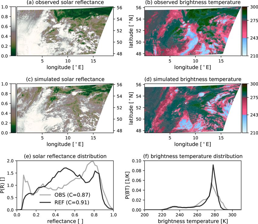
12274            S. Geiss et al.: Understanding the model representation of clouds based on visible satellite observations

cumulus, and Saharan dust outbreaks. Kurzrock et al. (2018)         tecting shortcomings related to model clouds (e.g. Tselioudis
also demonstrated that clouds, in particular the representa-        and Jakob, 2002; Otkin and Greenwald, 2008; Franklin et al.,
tion of low stratus in the model, dominate the uncertainty of       2013). These studies have shown that systematic cloud bi-
PV power production. Advances in the prediction of clouds,          ases are present in most models and that the representation
radiation and PV power generation are possible by improv-           of clouds depends on nearly every parameterisation in the
ing the representation of clouds in NWP models; this can be         model (Webb et al., 2001).
achieved by including more accurate physical parameterisa-             While quantities retrieved from satellite observations like
tions or tuning existing parameterisations related to clouds.       cloud optical depth are easier to interpret than the observa-
    Moreover, a good representation of clouds in NWP mod-           tions themselves, they have the drawback that characterising
els is also a prerequisite for assimilating cloud-related ob-       their errors is often problematic (Errico et al., 2007). Inter
servations, which improves the initial state from which fore-       alia, retrievals often incorporate model information leading
casts are started and, thus, also subsequent forecasts. Cloud-      to error correlations between the model and the retrieved in-
related observations like satellite images in the solar or ther-    formation used for evaluation. Therefore, in data assimila-
mal spectrum can only be assimilated if observed and simu-          tion, the “direct assimilation” of observations by means of
lated clouds exhibit a similar climatology. Unfortunately, this     forward operators is generally preferred over the assimilation
is not necessarily the case in current NWP systems (Gustafs-        of retrievals. A reasonable characterisation of errors is crucial
son et al., 2018; Tuohy et al., 2015). Therefore, understand-       not only for data assimilation but also for model evaluation.
ing and mitigating these systematic deviations will be an es-       Reliable conclusions can be drawn about model errors if the
sential ingredient for the operational assimilation of such ob-     errors in the evaluation method are sufficiently small.
servations. Some studies have already shown the benefit of             The aim of this study is to demonstrate the benefits of eval-
assimilating cloud-affected satellite radiances in the infrared     uating the representation of clouds in NWP models using a
(e.g. Geer et al., 2018; Honda et al., 2018) and in the visi-       combination of visible and infrared satellite images. Our re-
ble (Scheck et al., 2020) in experimental set-ups or idealised      sults are based on simulations with the ICON-D2 (ICOsa-
experiments (Schröttle et al., 2020). The assimilation led to       hedral Non-hydrostatic, development version based on ver-
significant improvements in cloud-related quantities and dy-        sion 2.6.1; Zängl et al., 2015) preoperational convection-
namical variables, as clouds are often associated with me-          permitting model of the Deutscher Wetterdienst (DWD; Ger-
teorologically sensitive areas (atmospheric instability) (Mc-       man Meteorological Service) for a highly convective sum-
Nally, 2002). However, current convection-permitting re-            mer period of 30 d over Germany and neighbouring areas.
gional NWP systems still do not assimilate cloud-affected           We will show that better insights into the origin of the sys-
satellite observations (Gustafsson et al., 2018), mainly due        tematic cloud errors can be gained using the two different
to systematic deviations.                                           satellite channels. Moreover, it will be demonstrated that this
    Cloud-related observations can also be used to diagnose         approach is also useful for assessing the impact of model
systematic errors in the model clouds and get information           changes aimed at reducing errors in the clouds and can, thus,
on which processes or parameterisations in the model need           directly support model tuning efforts.
to be improved. Satellite images obtained by instruments on            Given the advantages related to error characterisation, we
geostationary or polar-orbiting satellites are well-suited for      will follow the forward operator approach in this study and
this purpose, as they contain high-resolution information on        compare observed and synthetic images. For the genera-
the location and properties of clouds. As discussed in more         tion of synthetic infrared images, we will rely on the fast
detail in Sect. 2.2, the solar and thermal channels of these        methods available in the RTTOV (Radiative Transfer for
instruments provide complementary information on clouds’            TOVS) radiative transfer package (Saunders et al., 2018),
properties and can also depend, often in an ambiguous way,          which is operationally used by many weather centres (e.g. the
on the thermodynamic state of the atmosphere, aerosols and          European Centre for Medium-Range Weather Forecasts).
trace gases. In prior model evaluation studies, the satellite ra-   Several authors have examined the related uncertainties of
diance has often not been used, with researchers instead opt-       these methods (e.g. Senf and Deneke, 2017; Saunders et al.,
ing for easier to interpret quantities like cloud fraction, cloud   2017, 2018). For visible channels, we apply the newly de-
optical depth, and the cloud-top height derived from them           veloped VISible satellite image Forward OPerator (VISOP),
using retrieval algorithms (e.g. Zhang et al., 2005; Otkin and      which is based on the Method for Fast Satellite Image Syn-
Greenwald, 2008; Senf et al., 2020). These retrieved quan-          thesis (MFASIS) 1D radiative transfer method (Scheck et al.,
tities correspond directly to model variables or are closely        2016) and an extension to account for the most important
connected to them. The combination of information derived           3D radiative transfer (RT) effects (Scheck et al., 2018). The
from visible and infrared satellite observations like in the IS-    uncertainties of the visible forward operator will be discussed
CCP (International Satellite Cloud Climatology Project; see         in this study.
e.g. Rossow and Schiffer, 1991) approach that constructs               The remainder of the paper is structured as follows: the ex-
cloud type histograms of retrieved cloud optical thickness          perimental set-up is presented in Sect. 2. Two selected days
and cloud-top pressure has been particularly helpful for de-        with clouds on different levels are analysed in Sect. 3 to in-

Atmos. Chem. Phys., 21, 12273–12290, 2021                                           https://doi.org/10.5194/acp-21-12273-2021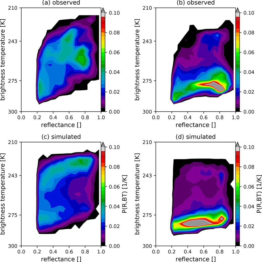
S. Geiss et al.: Understanding the model representation of clouds based on visible satellite observations                     12275

                                                                      such parameterisations could be further constrained by satel-
                                                                      lite observations. For this reason, we examine the sensitiv-
                                                                      ity of solar reflectances and infrared brightness temperatures
                                                                      (BTs) to variations in cloud-related parameterisations. We
                                                                      performed six additional simulations in which cloud-related
                                                                      parameterisations were modified within their range of uncer-
                                                                      tainty, i.e. using perturbed values that are physically plausi-
                                                                      ble. For this purpose, we modified the following four param-
                                                                      eterisations:
                                                                       1. The cloud droplet number concentration in ICON is
                                                                          used to calculate the cloud optical properties and the
                                                                          onset of precipitation. ICON employs the parameterisa-
Figure 1. ICON-D2 domain in the observation space (grey shading)
                                                                          tion of Segal and Khain (2006), which determines how
and the reduced evaluation domain (red box). The orange x sym-
                                                                          many droplets are in a cloud depending on an aerosol
bols indicate the DWD pyranometer stations that measure global
horizontal irradiance.                                                    number concentration derived from the climatology and
                                                                          on an updraught velocity at nucleation. The determina-
                                                                          tion of the updraught velocity in a 2km resolution model
troduce satellite observations and their characteristics. This is         is not straightforward because updraughts are under-
followed by a discussion of the cloud statistics for a full test          resolved. ICON assumes a constant updraught velocity,
period and associated systematic deviations. In Sect. 4, we               which serves as a control parameter: the number of nu-
assess the sensitivity of synthetic satellite images to model             cleated droplets increases with the updraught velocity.
and visible operator settings. For visible reflectances, for-
                                                                       2. The turbulent subgrid-scale cloud parameterisation de-
ward operator uncertainties and model sensitivity are com-
                                                                          termines the cloud cover due to the unresolved vari-
pared. Conclusions are provided in Sect. 5.
                                                                          ability in the model. The resulting turbulent cloud
                                                                          cover ccturb is combined with the detrainment cloud
2     Experimental set-up                                                 cover, which is given by a diagnostic approximation of
                                                                          the equivalent term in Tiedtke (1993). We focus on the
2.1    Model set-up and sensitivity experiments                           turbulent parameterisation of liquid clouds, as those are
                                                                          the main source of subgrid-scale clouds in the summer
To evaluate the cloud statistics during this period, we use               period chosen for the experiments.
the preoperational convection-permitting ICON-D2 (ICOsa-                   The turbulent cloud parameterisation in ICON for liq-
hedral Non-hydrostatic, development version based on ver-                  uid clouds is based on the assumption of an asymmet-
sion 2.6.1; Zängl et al., 2015) model configuration with                   ric probability distribution function (PDF) of total water
prescribed lateral boundary conditions (BCs) and a one-                    (including liquid and vapour). The cloud-cover function
way nesting. ICON-D2 replaced the operational COSMO-                       that is used starts from this assumption, but it has been
D2 (Consortium for Small scale-Modelling with a grid spac-                 empirically modified based on global and regional ex-
ing of 2.2 km) model (Baldauf et al., 2018). Simulations                   periments (Martin Köhler, DWD, personal communica-
over Germany (Fig. 1) with a horizontal grid spacing of                    tion, 2020). The final function reads
2.1 km and 65 vertical levels are initialised once on 26 May
2016 at 00:00 UTC from downscaled ICON-EU analysis ini-                    ccturb = ((qv + qc + A1q − qsat ) /(B1q))2 ,          (1)
tial conditions. ICON-EU analysis BCs drive this semi-free
simulation with an hourly update and a forecast horizon of                 where 1q is the variance of the total-water PDF and
30 d. The simulation period and domain size are sufficiently               is determined by the turbulence scheme; A and B are
large for the atmospheric model to develop its own cloud                   tunable parameters that are described below; and qsat
distribution without perturbations from data assimilation or               is the water vapour at saturation using the mean tem-
nudging. In our reference simulation, the operational single-              perature and pressure in the grid box. Some limiters
moment bulk microphysical parameterisation accounting for                  and resolution-dependent corrections are then applied
water vapour (qv ), cloud water (qc ), cloud ice (qi ), snow (qs ),        to achieve the final cloud fraction, but their description
rain (qr ) and graupel (qg ) is used (Lin et al., 1983; Reinhardt          is not relevant for this paper.
and Seifert, 2006).                                                        The parameter A determines the asymmetry of the size
   The reference preoperational model configuration has                    distribution: for larger A, clouds will be predicted at
been reached through extensive tuning of many parameters                   lower relative humidities, so the cloud cover will be
whose values are uncertain. As many of these parameteri-                   higher. This is a common tuning parameter when chang-
sations are related to clouds, it would be very beneficial if              ing the model configuration. For example, it is expected

https://doi.org/10.5194/acp-21-12273-2021                                           Atmos. Chem. Phys., 21, 12273–12290, 2021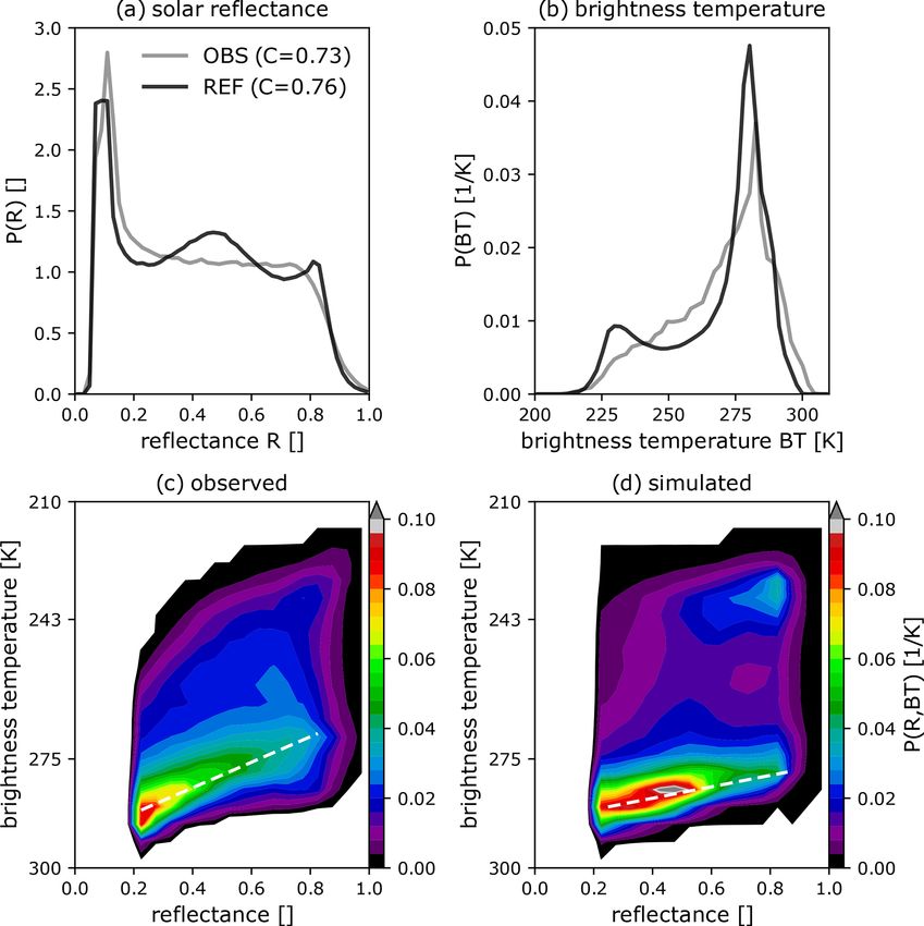
12276            S. Geiss et al.: Understanding the model representation of clouds based on visible satellite observations

     that the model requires less subgrid clouds as grid spac-     vii. Finally, we ran evaluated a two-moment scheme with
     ing is reduced and more clouds are resolved. The pa-               a strongly reduced asymmetry factor for subgrid-liquid
     rameter B was introduced in this study, and it scales the          clouds (A = 1.5, B = 2.5) and no subgrid ice clouds.
     cloud cover for a determined PDF asymmetry. Thus, it               This simulation was motivated by the fact that the two-
     allows for the cloud cover to be changed without mod-              moment scheme reflected too much radiation; therefore,
     ifying the relative humidities at which clouds are acti-           we reduced the amount of subgrid clouds.
     vated. In the preoperational configuration, these param-
     eters are set to A = 3.5 and B = 1 + A = 4.5.                 2.2   Satellite observations
 3. The shallow-convection parameterisation of Bechtold            The SEVIRI (Spinning Enhanced Visible InfraRed Imager)
    et al. (2014) predicts unresolved shallow convection in        instrument on board the Meteosat Second Generation (MSG)
    the model and also contributes to subgrid clouds. The          has eight channels in the solar and thermal part of the atmo-
    model limits the parameterisation to clouds that are suf-      spheric window, with a spatial resolution of 3 km × 3 km at
    ficiently thin, so that thicker clouds have to be resolved     the sub-satellite point and 6 km × 3 km in the ICON-D2 do-
    by the model. Thus, the thickness of the thickest non-         main. The temporal resolution is 15 min for full disc scans
    resolved cloud is an uncertain parameter that limits the       (Schmetz et al., 2002). In the solar regime, radiances are
    strength of the parameterisation.                              dominated by the scattering of photons from the Sun to
 4. The microphysical scheme describes the hydrometeors            the satellite sensor, whereas emission from the Earth’s sur-
    dynamics. We check the effect of using the two-moment          face and cloud top is dominant in the thermal. In this pa-
    parameterisation of Seifert and Beheng (2006), in which        per, we use the visible 0.6 µm channel (VIS006), which has
    the number concentrations of different variables are           the advantage that the surface albedo is usually relatively
    treated as prognostic variables. This is a more com-           low (R < 0.15) at this wavelength; thus, errors in the albedo
    plex scheme and can potentially simulate more realis-          at the above-mentioned wavelength are smaller than for the
    tic clouds. However, the two-moment scheme has never           0.8 µm channel (VIS008) that would also be available from
    been tuned like the operational one-moment scheme.             SEVIRI. Additionally, we use the 10.8 µm thermal infrared
                                                                   window channel (IR108). At this wavelength, the signal is
  In order to investigate the sensitivity of satellite synthetic   not strongly affected by gaseous absorption within the at-
observations to these parameterisations, we evaluated seven        mosphere and is mainly determined by emission from the
simulations:                                                       ground and clouds at all heights. For a better understanding
                                                                   and interpretation of our results, we discuss the sensitivity
  i. First, a reference simulation with preoperational model       of the VIS006 and IR108 signals to the liquid and ice wa-
     configuration was evaluated.                                  ter paths (LWP and IWP respectively), as shown in Fig. 2.
 ii. We then increased the cloud droplet number concen-            The signals are computed using DISORT (DIScrete Ordi-
     tration by increasing the updraught velocity at activa-       nates Radiative Transfer; Stamnes et al., 1988) for idealised
     tion (from 0.25 to 1 m s−1 ). This produces liquid clouds     scenes with a single-layer water cloud at a height of 4 km or
     that are optically thicker, as the number concentration       a single-layer ice cloud at a height of 10 km.
     of droplets increases roughly by a factor of 3.                  Both solar reflectance and infrared brightness tempera-
                                                                   ture strongly depend on the LWP and IWP, although in dif-
 iii. Next, we modified the distribution of turbulent subgrid      ferent ranges: VIS006 is most sensitive to LWP/IWP val-
      liquid clouds. The idea was to produce less and thicker      ues in the [10−2 , 100 ] kg m−2 range, whereas the sensitiv-
      subgrid clouds in a way that the radiative balance of the    ity of IR108 is limited to thinner clouds with values in
      model remained unchanged. This was achieved after a          the [10−2 , 10−1 ] kg m−2 range due to fast saturation of
      few trial-and-error experiments by using the parameters      the signal by the absorption of photons. Figure 2b implies
      A = 2.5 and B = 0.21.                                        that only cloud-top height and its corresponding tempera-
                                                                   ture determines the observed BT for a single-layer water
 iv. A stronger shallow-convection parameterisation was            cloud with LWP > 0.03 kg m−2 or a single-layer ice cloud
     then evaluated by doubling the thickness of the thick-        with IWP > 0.1 kg m−2 . Hence, the IR signal can provide
     est unresolved cloud (from 2 × 10⁴ to 4 × 10⁴ Pa).            the cloud-top temperature but does not allow for retrieval
  v. We then evaluated a simulation with the two-moment            of the LWP/IWP. In contrast, the solar reflectance is only
     scheme while all other parameterisations remained             0.35 at these threshold values and can still provide infor-
     equal to the operational configuration.                       mation on the water/ice content up to LWP/IWP values of
                                                                   about 1 kg m−2 . These different and complementary sensi-
 vi. Following this, we ran a two-moment scheme in which           tivities show that model evaluation with solar and thermal
     the subgrid-cloud parameterisation for ice clouds was         channels has the potential to provide more information on
     switched off.                                                 the nature of the systematic errors and to possibly identify

Atmos. Chem. Phys., 21, 12273–12290, 2021                                         https://doi.org/10.5194/acp-21-12273-2021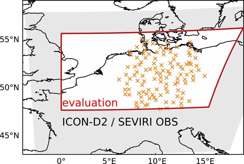
S. Geiss et al.: Understanding the model representation of clouds based on visible satellite observations                                   12277

Figure 2. Water and ice cloud signals with different effective particle radii from 0.6 µm SEVIRI solar reflectance (VIS006) (a) and 10.8 µm
SEVIRI brightness temperature (IR108) (b), computed using DISORT. Dashed lines indicate saturation in IR108 for water (red) and ice
(blue) clouds. The albedo was set to 0.1, the solar zenith angle was set to 30◦ , the satellite zenith angle was set to 60◦ and the scattering angle
was set to 135◦ .

specific shortcomings that would not be visible by only ex-                 MFASIS is based on a compressed lookup table (LUT), com-
amining a single channel.                                                   puted using the DISORT solver, where the aerosol optical
   An interesting consequence of these different sensitivities              depth (AOD) is assumed to be zero. However, it is possible to
is that one would expect visible reflectance to provide more                consider aerosols or different kinds of ice habits for the com-
information on the transmittance of solar radiation to the sur-             putation of the MFASIS LUT (results in Sect. 4.2). VISOP
face than infrared radiances, as this process depends strongly              takes the slant satellite viewing angle into account (tilted in-
on the water content of the clouds. Therefore, visible re-                  dependent column approximation; Wapler and Mayer, 2008)
flectances should be more strongly correlated with the in-                  and accounts for the most important 3D RT effect by us-
coming radiation at the surface than infrared brightness tem-               ing the cloud-top inclination correction (CTI) described in
peratures. This is confirmed by Fig. 3, which displays the                  Scheck et al. (2018). The surface albedo values required as
correlations between the observed signals of the two satellite              input for MFASIS are taken from the RTTOV BRDF atlas
channels and normalised hourly averages of the global hori-                 (Vidot et al., 2018).
zontal irradiance (GHI) measured at 122 DWD pyranometer                        As we aim to achieve consistent assumptions in both the
stations (Fig. 1). There is indeed a strong negative correla-               operator and the NWP model, we decided to use effective
tion between the visible reflectance and the surface radiation,             radii from the microphysics for water clouds directly. This
with a correlation coefficient ρobs = −0.75 (Fig. 3a). The                  is based on the consideration that radiative transfer, micro-
anticorrelation is strong but not perfect due to the follow-                physics and possibly operators should deal with the same op-
ing reasons: (1) the instantaneous solar reflectance is com-                tical properties.
pared to the time-averaged quantity GHI, (2) reflectance is                    However, some adjustments are required for the ice
averaged over pixels but GHI is a point measurement, and                    clouds, as will be motivated in the following. The micro-
(3) 3D radiative transfer effects modify reflectance and GHI                physics scheme in the simulation predicts six hydrometeor
in different ways. For constant water content, surface radi-                categories: cloud water, cloud ice and precipitating liquid
ation should not be strongly correlated with the cloud-top                  water, snow, hail, and graupel. Rain droplets, hail and graupel
height or temperature. However, as many high clouds are                     particles are assumed to be much larger than cloud droplets
caused by convection and these clouds contain large amounts                 and cloud ice particles in the model. Therefore, for the same
of water, there is also some correlation between brightness                 mass, they are also much less effective at scattering radiation
temperature and surface radiation (Fig. 3b), but it is weaker               and are, thus, neglected in the forward operators. However,
(ρobs = 0.62) than for the visible reflectances. These results              the distinction between snow and cloud ice particles in the
indicate that by reducing the error of synthetic satellite im-              model is rather artificial. Model snow particles can be small
ages, in particular for visible satellite channels, it should be            enough to cause non-negligible scattering effects (see discus-
possible to improve radiation forecasts.                                    sion in Hogan et al., 2001). Hence, as a (first) approximation,
                                                                            we construct a frozen phase whose total mass, qitot , is the sum
2.3   Satellite forward operators                                           of the diagnosed ice water content (grid- and subgrid-scale)
                                                                            and snow content (only grid scale available) and whose “ef-
To compute model equivalents for visible satellite images                   fective effective radius”,
from the ICON model state, we employ the VISible satel-
lite image Forward OPerator (VISOP) that uses the MFA-                       tot                 qitot
                                                                            ri,eff =                                ,                          (2)
SIS 1D radiative transfer (RT) method (Scheck et al., 2016).                           qidia /ri,eff + qs /rs,eff

https://doi.org/10.5194/acp-21-12273-2021                                                    Atmos. Chem. Phys., 21, 12273–12290, 2021
12278             S. Geiss et al.: Understanding the model representation of clouds based on visible satellite observations

Figure 3. The 0.6 µm SEVIRI solar reflectance (VIS006) (a) and 10.8 µm SEVIRI brightness temperature (IR108) (b) against the fraction of
incoming global horizontal irradiance (GHI/(cos(sza)E0 )) at 12:00 UTC. Here, E0 (solar constant) is assumed to be 1367 W m−2 , and the
number of co-located observations at pyranometer stations is 3365.

is defined using the simulated effective radii of cloud ice ri,eff    in the RTTOV 12.1 package (Saunders et al., 2018), which is
and snow rs,eff . The effective radii for ice and snow are cal-       used by many weather services.
culated under the assumption that both hydrometeors behave               For the evaluation, we applied both operators at the full
as randomly oriented needles, and using the mass–size rela-           model resolution and interpolated solar reflectances and the
tionships, size distributions and number concentrations from          brightness temperature to the observation space afterwards
the microphysics (for details, see Fu et al., 1997, and Muska-        to avoid additional representativeness errors (Marseille and
tel et al., 2021). This approximation assumes that the optical        Stoffelen, 2017).
thickness of the frozen phase is equal to the sum of the optical
thicknesses of the ice and snow phases, similar to the work of        2.4   Evaluation metrics
Senf and Deneke (2017). The approximation becomes exact
in the case of wavelengths much smaller than the hydrome-             A combination of metrics is applied to evaluate synthetic
teors’ size (optical limit); therefore, it is quite appropriate for   satellite imagery at 12:00 UTC with observations. The eval-
visible channels.                                                     uation domain (red rectangle in Fig. 1) is smaller than the
   In general, we use the diagnosed cloud water content and           ICON-D2 domain to exclude nesting effects at the domain
ice content including subgrid contributions as input for VI-          boundaries and signals from snow-covered surfaces in the
SOP. If no subgrid-scale cloud is diagnosed in a particular           Alps that exhibit reflectances similar to clouds. We show
grid box, qxdia = qx , where x could be either water or ice. We       the VIS006 and IR108 probability density functions of our
assume no differences in the microphysical and optical prop-          simulations and observations P (R). The number of bins N
erties of grid and subgrid clouds, so that the effective radius       of the PDFs is 50, with R ∈ [0, 1] and BT ∈ [200, 310] K.
calculation is the same for both cases.                               From that, we define the cloudiness (C) as the fraction of
   An accurate calibration is a prerequisite for using satel-         pixels in which the solar reflectance is higher than a thresh-
lite observations, but unfortunately the calibration of SE-           old value Rc of 0.2. This value is an upper limit for the
VIRI VIS006 is uncertain. Meirink et al. (2013), for ex-              clear-sky reflectance in the considered evaluation domain
ample, found a bias of −8 % for VIS006 during the pe-                 (see discussion in Scheck et al., 2018). Violin plots are used
riod from 2004 to 2008 by comparing MSG SEVIRI and                    to visualise the daily bin-by-bin deviation of the PDF (de-
MODIS (Moderate Resolution Imaging Spectroradiometer)                 viation computed for each day d and bin n) from the refer-
                                                                                                                              PDF =
                                                                      ence run and model/operator sensitivity experiments: n,d
Aqua observations. For our purpose, we use the approach to
                                                                             obs        sim
                                                                      P (R)n,d − P (R)n,d . This allows for a consistent comparison
find a suitable bias correction by minimising the average his-
togram difference between the observed and simulated solar            of VISOP and model uncertainty by examining the median
reflectance distribution. Through this, we found a deviation          deviation (the mean is always zero), the interquartile range
of −13 % between observations and our reference simula-               (difference between 75th and 25th percentile) as a measure of
tion, which can be partly contributed to a calibration offset         variability and the range as the extent of deviations. We fur-
(observations too dark) and a model bias.                             ther analyse clouds by constructing contoured 2D PDF plots
   To derive SEVIRI infrared brightness temperature from              of brightness temperature and solar reflectance, comparable
the model state, we use the efficient methods implemented             to the ISCCP approach (Rossow and Schiffer, 1991) or to
                                                                      contoured frequency by altitude diagrams (CFADs; Yuter and

Atmos. Chem. Phys., 21, 12273–12290, 2021                                              https://doi.org/10.5194/acp-21-12273-2021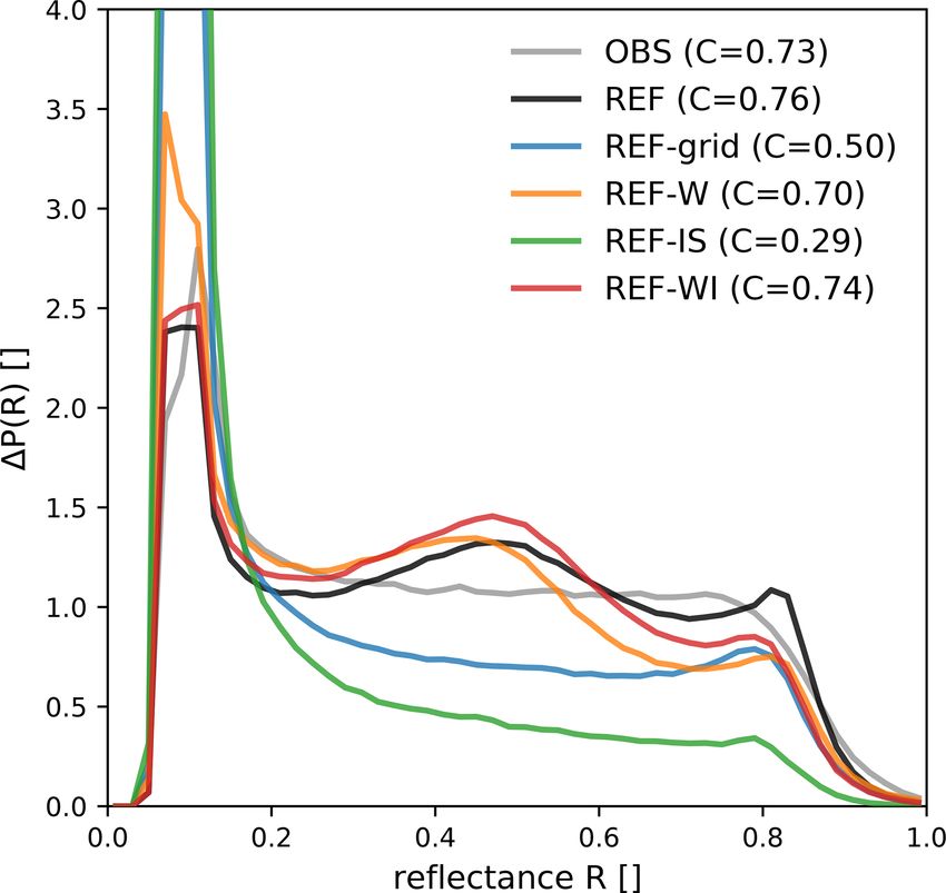
S. Geiss et al.: Understanding the model representation of clouds based on visible satellite observations                      12279

                                                                      3     Reference run

                                                                      3.1    Selected cases

                                                                      In this section, we discuss 2 d of the period to illustrate
                                                                      the methodology for evaluating clouds using visible and in-
                                                                      frared satellite channels. On the first day (29 May), deep
                                                                      convection and severe thunderstorms occurred, leading to a
                                                                      flash flood that caused severe damage in Braunsbach, a small
                                                                      town in the south-western part of Germany. The second day
                                                                      (2 June) was dominated by low-level clouds. According to
                                                                      Piper et al. (2016), warm, moist and unstable air masses char-
                                                                      acterised both days. However, large-scale ascent dominated
                                                                      on 29 May and subsidence dominated on 2 June. Figure 5
Figure 4. Time series of observed and simulated cloudiness at         shows the VIS006 and IR108 satellite images as well as the
12:00 UTC during the period from 26 May to 24 June 2016. The          corresponding distributions of solar reflectance and bright-
cloudiness is defined as the fraction of pixels where 0.6 µm SEVIRI   ness temperatures on 29 May 2016. The VIS006 satellite im-
solar reflectance R > 0.2.                                            age (Fig. 5a, c) shows the early stage of a cyclogenesis over
                                                                      Germany, characterised by a prominent vortex structure in
                                                                      both the observations and model simulation. However, the
Houze, 1995) of radar observations. We use the US Standard            feature is shifted to the south-west in the simulation. The rel-
Atmosphere 1962 (Sissenwine et al., 1962) to classify bright-         atively high cloudiness of 88 % in the observations and 89 %
ness temperatures into three cloud categories (low, middle            in the simulation leads to a relatively uniform distribution of
and high clouds) as defined in the International Cloud Atlas          observed solar reflectances (Fig. 5e). Overall, the agreement
(Cohn, 2017). In the US Standard Atmosphere, the surface              between observed and simulated visible histograms is rela-
temperature is 288 K and the (wet) temperature lapse rate is          tively good given that the model is forced towards the current
0.65 K/100 m, leading to temperature ranges of T > 275 K              weather only through the boundary conditions. The vortex
for the surface and low clouds, 275 K ≤ T ≤ 243 K for mid-            structure of the cyclogenesis is also apparent in the IR108 ob-
dle clouds, and T < 243 K for high clouds.                            servations (Fig. 5b), but the simulation shows clear system-
                                                                      atic errors. In the simulation, the cloud pattern is dominated
2.5   Synoptic overview and cloudiness
                                                                      by relatively high ice clouds (Fig. 5d), which are less fre-
A 30 d period from 26 May to 24 June 2016 is analysed,                quent in the observations. The histogram confirms this pic-
which is dominated by strong summertime convection in                 ture: the signal of high clouds is overestimated in the simula-
Germany. In the beginning, large parts of Europe were af-             tions, whereas the signal of medium clouds is underestimated
fected by high-impact weather events over almost 2 weeks.             by 40 %.
Atmospheric blocking and the interaction of low thermal sta-             On 2 June 2016, boundary layer clouds dominated in
bility and weak mid-tropospheric winds were the ingredients           both the observations and simulation (Fig. 6b, d). Addition-
for this exceptional sequence of thunderstorms and related            ally, superimposed ice clouds are observed in some regions.
flash floods (Piper et al., 2016). Many authors have discussed        The simulated IR108 distribution fits the observed one rela-
these 2 weeks (see e.g. Necker et al., 2020; Bachmann et al.,         tively well on this day (Fig. 6f). In the visible satellite im-
2020; Keil et al., 2019; Necker et al., 2018; Zeng et al., 2018).     age (Fig. 6a, c), a high cloudiness is apparent, with 87 % in
In the subsequent weeks (10–24 June), the wind direction              the observations and 91 % in the simulation. In contrast to
changed to a south-westerly flow, advecting warm and hu-              29 May, however, the distribution (Fig. 6e) reveals an over-
mid air masses from the Atlantic and the Mediterranean to             estimation of medium thick clouds as well as an underesti-
Germany and supporting cloud formation (Fig. 4). In gen-              mation of thick clouds (R > 0.6).
eral, the simulated cloudiness (defined in Sect. 2.4) is pre-            The examples discussed above show that the examina-
dominantly overestimated, leading to a mean observed and              tion of a single channel (VIS or IR) can lead to opposite
simulated cloudiness for the period of 0.73 and 0.76 respec-          conclusions with respect to forecast quality. The agreement
tively. This convective period with high cloud cover at dif-          of the histograms for 29 May is good in the visible range
ferent levels is well-suited to examine cloud statistics and its      but not in the IR; the opposite is observed for the 2 June.
sensitivity to cloud-related parameterisations.                       This shows that both channels provide complementary infor-
                                                                      mation. In the following, we show that further information
                                                                      can be obtained by using the combined information of both
                                                                      channels in 2D PDF plots of brightness temperature and re-
                                                                      flectance. We have already discussed how the IR histogram

https://doi.org/10.5194/acp-21-12273-2021                                           Atmos. Chem. Phys., 21, 12273–12290, 2021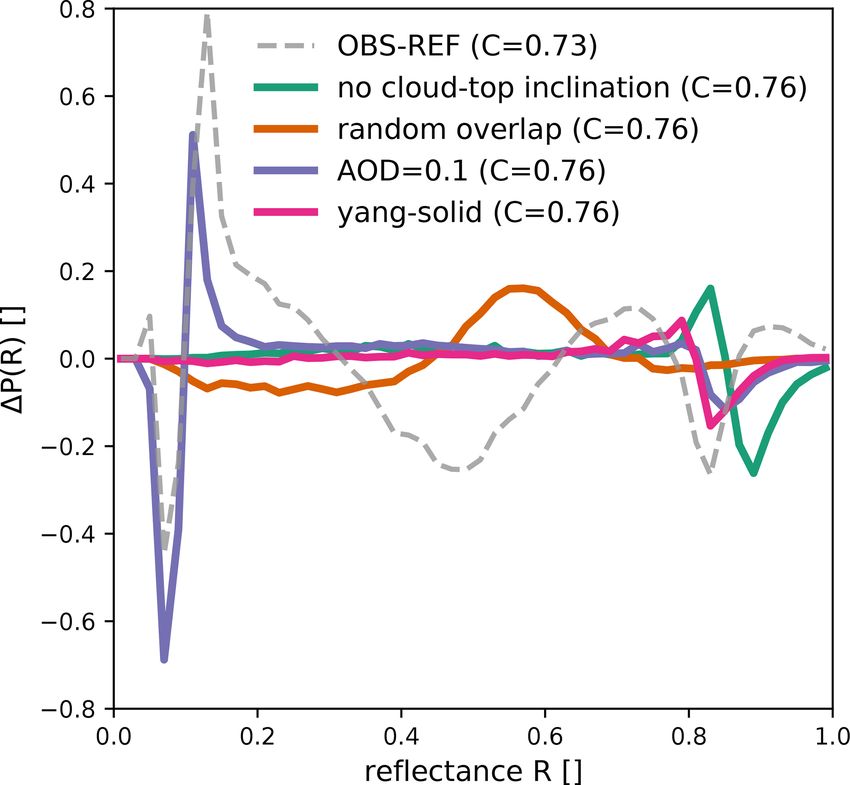
12280 S. Geiss et al.: Understanding the model representation of clouds based on visible satellite observations
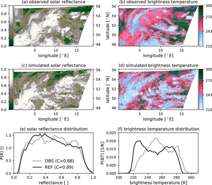
Figure 5. The (regional) distribution of 0.6 µm SEVIRI solar reflectance (a, c, e) and 10.8 µm SEVIRI brightness temperature (b, d, f) as
well as their corresponding distribution for 29 May at 12:00 UTC. The numbers in the legend of panel (e) indicate the cloudiness, i.e. the
fraction of pixels exceeding a reflectance of 0.2 (EUMETSAT).
shows an overestimation of high clouds on the 29 May. The 3.2 VIS006 and IR108 statistics for the full period
combined histograms (Fig. 7a, c) provide the additional in-
formation that this overestimation of clouds mostly happens
The analysis of individual cases presented above illustrates
for thick clouds (R > 0.6). This indicates that the model pro-
certain characteristics, but longer periods are required to
duced overly strong deep convection. On 2 June, where lower
identify systematic model deficiencies. To address this, we
clouds dominated the scene, the observations and simulations
now present results for the 30 d period. The observed mean
agree on the vertical location of the shallow cumulus clouds
VIS006 solar reflectance distribution at 12:00 UTC reveals
(Fig. 7b, d). However, solar reflectances are primarily dis-
a clear-sky peak at low reflectance values (R ∈ [0, 0.2]),
tributed around 0.7 in the observations and around 0.5 in the
a nearly uniform distribution for higher reflectances (R ∈
simulation. Compared with the 1D reflectance histogram, the
[0.2, 0.8]) and a sharp decrease for reflectances higher
2D PDF provides the additional information that the system-
than 0.8 (Fig. 8a). The distribution of the reference simula-
atic reflectance errors are related to low clouds. These 2 d
tion overall looks similar, but it shows some deviations from
with predominantly deep convective clouds (29 May) and
the flat plateau seen for the observations, with a surplus of
low clouds (2 June) are for different cloud types and forma-
clouds around a reflectance of 0.5. Figure 8b presents a his-
tion processes. Thus, their analysis illustrates the benefit of
togram of the 30 d mean IR108-BT at 12:00 UTC. There are
combining a visible and an infrared channel.
generally too many clouds with low brightness temperatures
(BT < 240 K). This, along with an underestimation of mid-
level clouds in our ICON simulations, is a well-known issue
that has been found for many global circulation or weather
prediction models using forward operators or retrievals for
Atmos. Chem. Phys., 21, 12273–12290, 2021 https://doi.org/10.5194/acp-21-12273-2021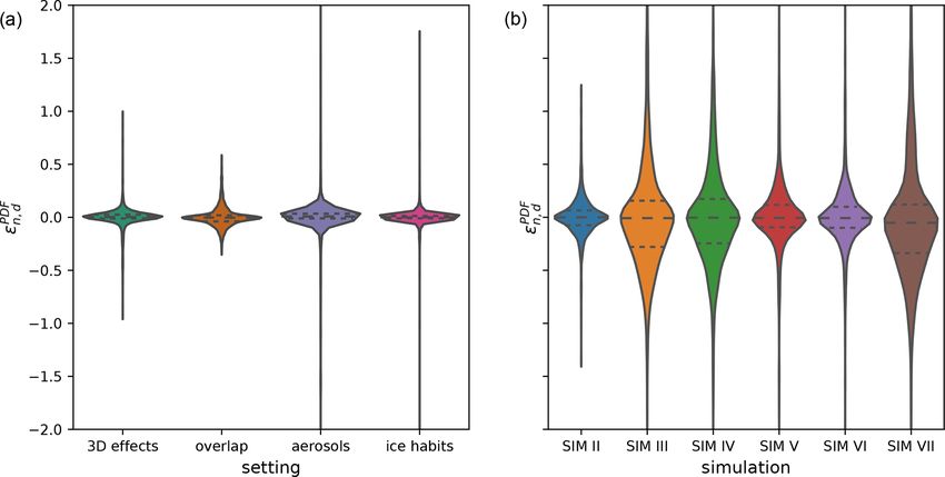
S. Geiss et al.: Understanding the model representation of clouds based on visible satellite observations                              12281

Figure 6. The (regional) distribution of 0.6 µm SEVIRI solar reflectance (a, c, e) and 10.8 µm SEVIRI brightness temperature (b, d, f) as
well as their corresponding distribution for 2 June 2016 at 12:00 UTC. The numbers in the legend of panel (e) indicate the cloudiness, i.e. the
fraction of pixels exceeding a reflectance of 0.2 (EUMETSAT).

evaluation (e.g. Illingworth et al., 2007; Pfeifer et al., 2010;          water clouds. In addition, the simulation does not produce
Böhme et al., 2011; Franklin et al., 2013; Keller et al., 2016).          enough mid-level clouds at all solar reflectances. Finally, a
Zhang et al. (2005) discussed possible reasons for the lack of            secondary maximum at low BTs and high solar reflectance
mid-level clouds and concluded that physical deficiencies in              (R ≈ 0.8) is apparent in the simulations but not in the obser-
the model might introduce these systematic deviations. The                vations. This maximum mainly corresponds to deep convec-
distribution further reveals a clear-sky bias, where the model            tive and precipitating clouds, which are either too active or
underpredicts high BT values.                                             produce too much ice, similar to 29 May. High-level clouds
   In general, the statistics for the full period, as shown by            (cirrus as well as iced cloud tops) and low-level clouds are
the 2D PDFs in Fig. 8c and d, indicates that the model and                generally overestimated.
observation distributions have similar structures. Noticeable                The combined histograms clearly show important short-
differences in the distribution occur in boundary layer clouds.           comings in shallow and deep convection. Thus, combined
The increase in solar reflectance with decreasing brightness              histograms can provide additional information on the na-
temperature (increasing height) is noticeably steeper in the              ture of the systematic errors evident in the 1D histograms
observations (indicated by dashed white lines in the plots).              as well as very valuable information for model development,
This means that thick boundary layer clouds consistently                  showing which model configuration produces more realistic
reach higher levels in the observations and suggests that shal-           clouds.
low convection is too weak in the model. The 2D PDFs fur-
ther indicate that the surplus of clouds around a reflectance
of 0.5 in the model is related to boundary layer clouds, re-
vealing a deficiency in the model representation of liquid

https://doi.org/10.5194/acp-21-12273-2021                                                 Atmos. Chem. Phys., 21, 12273–12290, 2021
12282             S. Geiss et al.: Understanding the model representation of clouds based on visible satellite observations

Figure 7. Combined 0.6 µm SEVIRI solar reflectance (VIS006) and 10.8 µm SEVIRI brightness temperature (IR108) PDF of observa-
tions (a, b) and simulations (c, d) on 29 May (a, c) and 2 June 2016 (b, d) at 12:00 UTC.

4     Sensitivity of synthetic VIS006 and IR108 satellite        question. Cloudiness values C are provided for each case in
      observations                                               Fig. 9 to better quantify the relative importance of different
                                                                 cloud contributions.
4.1    Contributions of different clouds to the reflectance         Grid-scale clouds only lead to a distribution with a nearly
       distribution                                              flat plateau between reflectances of 0.3 and 0.7, a feature
                                                                 that is also found in the distribution of the observed re-
To better understand the sensitivity of the synthetic visible    flectances. However, the fraction of cloud pixels would de-
satellite images to changes in operator settings and model       crease from C = 0.76 to 0.5 if only grid-scale clouds were
modifications, it is helpful to determine the contribution of    present. Adding subgrid clouds results in much better agree-
different hydrometeor types and subgrid-scale clouds to the      ment with the observed value of C = 0.73. It is, thus, es-
reflectance histogram of the reference run (Fig. 8a). Figure 9   sential to take these additional subgrid clouds into account.
shows the observed and simulated VIS006 solar reflectance        However, the imperfect parameterisation of subgrid clouds
distribution (OBS and REF are the same as in Fig. 8a), the       also contributes to deviations in the shape of the distribution:
distribution that results from taking only grid-scale clouds     while the distributions of the observations and the grid-scale-
into account (REF-grid) and several distributions obtained       clouds-only simulation exhibit a relatively flat plateau, the
by using only certain types or combinations of hydromete-        addition of subgrid clouds leads to a histogram curve with a
ors. By comparing the contribution of a certain cloud type,      pronounced maximum at 0.5 and a minimum at 0.7.
e.g. REF − REF-grid for the subgrid clouds, to the deviation        When only water clouds are used as input to the opera-
of REF from OBS, one can infer if tuning (i.e. slightly chang-   tor (REF-W), the cloudiness falls off from C = 0.76 to C =
ing) parameters related to this cloud type in the model or the   0.70. Primarily, reflectances larger than 0.5 become slightly
operator could be helpful to reduce REF − OBS. The shapes        less frequent. In contrast, taking only ice clouds (including
of the curves can provide further information regarding this

Atmos. Chem. Phys., 21, 12273–12290, 2021                                        https://doi.org/10.5194/acp-21-12273-2021
S. Geiss et al.: Understanding the model representation of clouds based on visible satellite observations 12283
Figure 8. Individual PDFs for 0.6 µm SEVIRI solar reflectance (VIS006) (a), 10.8 µm SEVIRI brightness temperature (IR108) (b) and
combined VIS006–IR108 PDF (c, d) of observations (c) and simulations (d) at 12:00 UTC for the full test period. The numbers in the legend
of panel (a) indicate the cloudiness, i.e. the fraction of pixels exceeding a reflectance of 0.2.
snow) into account (REF-IS) has a more substantial impact 4.2 Estimated uncertainty of VISOP
on the histogram and results in a much smaller cloudiness of
C = 0.29. Thus, water clouds play a much more substantial Forward operators use fast, approximate RT methods and
role in the reflectance distribution than ice clouds. This re- rely on the limited information that is available from the
sult is not surprising, as the ice water path is much smaller NWP model. Due to missing 3D RT effects and missing in-
than the liquid water path, and larger ice particles are also formation (e.g. on unresolved cloud properties), their output
less effective at scattering light than smaller water droplets is to some extent uncertain. While forward operators for ther-
(Fig. 2a). mal infrared channels have been available for some time and
In both the water-only and the ice-only cases, the cor- their uncertainties have been investigated in several studies
responding subgrid clouds are included. The water-only (e.g. Senf and Deneke, 2017; Saunders et al., 2017, 2018),
curve (REF-W) shows the same deviation from the plateau- no such information is available for visible channels. In the
like shape of the observed distribution as the curve computed following, the uncertainty related to what we regard as the
for all clouds (REF), but the ice-only curve (REF-IS) does most critical error sources will be estimated by varying the
not. Thus, it seems that the subgrid water cloud parameter- corresponding operator settings.
isation needs to be improved to get better agreement in the The potential sources of uncertainty to be investigated are
histogram shapes. Finally, ignoring the simulated snow con- related to missing 3D RT effects, unknown or inconsistent
tent (REF-WI) has a small but detrimental effect. This em- overlap statistics of subgrid-scale clouds, the spatial and tem-
phasises the need to include snow in the computation of the poral variation of aerosols, and the shape of cloud ice parti-
RT input variables, as discussed in Sect. 2.3. cles. To estimate the upper limits of the uncertainty in the
reflectance distribution related to these sources, we repeated
the computation of visible reflectances applying VISOP to
https://doi.org/10.5194/acp-21-12273-2021 Atmos. Chem. Phys., 21, 12273–12290, 202112284 S. Geiss et al.: Understanding the model representation of clouds based on visible satellite observations
Figure 9. The 0.6 µm SEVIRI solar reflectance histograms for the Figure 10. Differences between the 0.6 µm SEVIRI solar re-
test period computed for the observations (OBS) and the refer- flectance PDFs obtained for the reference run with modified op-
ence experiment (REF). The additional distributions were com- erator settings and standard settings. The modified settings are
puted using only the grid-scale clouds (REF-grid), only the water switching off the cloud-top inclination, using random instead of
clouds (REF-W) and only the ice clouds (REF-IS) of the reference maximum-random subgrid cloud overlap, including aerosols with
experiment respectively. For the red line (REF-WI), water and ice an optical depth of 0.1 and changing the cloud ice particle habit to
clouds are taken into account, and only the snow contribution to solid columns. For comparison, the difference between the observa-
the ice clouds is omitted. The numbers in the legend indicate the tions and the reference run histogram is also shown (dashed curve).
cloudiness, i.e. the fraction of pixels exceeding a reflectance of 0.2.
top surface tilted towards the Sun appear brighter, and those
the reference simulation with deactivated cloud-top incli- tilted away from the Sun appear darker. The cloud-top incli-
nation (CTI) parameterisation, random instead of random- nation correction (CTI; see Scheck et al., 2018) accounting
maximum subgrid cloud overlap, and aerosols or a differ- for this effect has been shown to reduce the error with respect
ent kind of ice habit included in the MFASIS LUT. The to full 3D RT calculations and is included in the reference
deviations in the reflectance distribution for the reference run. The main effect of the CTI on the reflectance histogram
run caused by changing these operator settings are shown in is to reduce the slope at the high-reflectance end of the distri-
Fig. 10. bution and to bring it in better agreement with observations.
The subgrid cloud overlap assumptions would not be a Switching off the CTI leads to an overly steep decline of the
source of operator uncertainty if the assumptions in the NWP distribution at high reflectances, which is visible as a double-
model and the operator were entirely consistent. However, peak structure at R > 0.8 in Fig. 10. Other 3D RT effects like
the near-operational version of ICON employed to perform cloud shadows may also play a role, in particular for larger
the model runs for this study uses inconsistent overlap as- zenith angles. However, by focusing on observations near lo-
sumptions in the infrared and visible part of the spectrum. cal noon, their influence should be minimised.
This inconsistency will likely be corrected in future ver- According to retrievals based on measurements at
sions, but at the moment, it means that the operator can- AERONET (AErosol RObotic NETwork) stations (see Giles
not be entirely consistent with the model. The deviation in et al., 2019) in Germany, the mean AOD in June 2016 was in
the reflectance distribution caused by changing the assump- the range of 0.06 to 0.12 at a wavelength of 675 nm, which
tion from maximum-random to random in the operator (or- is similar to the wavelength of the visible channel consid-
ange line in Fig. 10) can be regarded as an upper limit for ered here. To estimate the impact of these aerosols on the
the impact. Changing the assumption shifts the peak around reflectance histogram, an MFASIS LUT was computed that
R = 0.5 (which is related to subgrid clouds, as discussed in includes aerosols (the “continental clean” aerosol mixture
Sect. 4.1) to higher reflectances but does not have much in- available in libRadtran; see Emde et al., 2016) with an optical
fluence on reflectances larger than 0.7. depth of 0.1. Including aerosols in the MFASIS LUT (i.e. tak-
Missing or imperfectly modelled 3D RT effects are likely ing direct aerosols effect into account) influences the re-
the source of uncertainty that is most difficult to quantify. Ac- flectance histogram in two ways. Under clear-sky conditions,
cording to Scheck et al. (2018), the most important 3D effect the reflectance increases because aerosols scatter photons to
is related to the inclination of the cloud-top surface, which the satellite, whereas under cloudy conditions, aerosols scat-
influences the observed reflectance. The parts of the cloud- ter photons out of their path towards the satellite. Thus, in
Atmos. Chem. Phys., 21, 12273–12290, 2021 https://doi.org/10.5194/acp-21-12273-2021S. Geiss et al.: Understanding the model representation of clouds based on visible satellite observations 12285
the presence of aerosols, the high-reflectance end of the dis- creases from 0.76 to 0.8, which means that the deviation from
tribution is shifted towards lower reflectances, and the low- the observed value of 0.73 is considerably larger.
reflectance end is shifted towards higher reflectances. Shift- Switching to the double-moment microphysics scheme
ing the pronounced ground peak in the distribution causes a (experiment V) mainly moves pixels with very high re-
double-peak structure at low reflectances in Fig. 10, whereas flectances (R > 0.8) to somewhat lower reflectance values
shifting the flat high-reflectance end only causes a single neg- between 0.6 and 0.8 and increases the cloudiness slightly.
ative peak. In general, the error introduced by direct aerosol Thin to intermediate clouds (0.2 < R < 0.6) are only weakly
effects for events like (Saharan) dust outbreaks can be higher affected. Still using the two-moment scheme but turning off
and could potentially lead to significant errors in solar re- subgrid-scale ice clouds (experiment VI) slightly decreases
flectances. Thus, days affected by such events, which did not the cloudiness but basically leads to the same distribution
occur during our test period, should be excluded from model as experiment V. Hence, ice subgrid-scale clouds cannot be
evaluation studies. responsible for the surplus of pixels with solar reflectances
Finally, the shape of cloud ice particles is also an uncertain around R = 0.5 that was attributed to subgrid clouds in
factor that influences the reflectances’ distribution. Changing Sect. 4.1. Finally, reducing the subgrid-scale water clouds
the shapes quite strongly from the baum_v36 general habit (experiment VII) also leads to much larger changes, with
mixture (Baum et al., 2014) to solid columns (using the op- negative peaks around R = 0.5 and R = 0.8 and positive val-
tical properties of Yang et al., 2005) basically only affects ues for R < 0.35. These changes point in the right direction
the highest reflectances, which are slightly reduced. Hence, with respect to mitigating the deviations of the reference run
the ice habit is not likely to cause large uncertainties in the (dashed line in Fig. 11a). However, the modification is too
reflectance distribution for our test period, which is charac- strong here, as cloudiness is dramatically underpredicted in
terised by a high low-level cloud cover and overlaying semi- this case (C = 0.64). Compared with visible reflectances, the
transparent cirrus clouds. For periods with more and thicker changes in the BT distribution introduced by modified model
ice clouds, the uncertainties could be higher. settings are more difficult to interpret because the signal de-
pends on cloud optical depth as well as on cloud-top height.
The modifications in experiments II and III only affect water
4.3 Sensitivity to model settings
clouds and, thus, only lead to changes at higher BTs. These
changes are relatively small compared with those required
Figure 11 shows the deviations of the reflectance and BT dis- to correct the deviations in the reference run (dashed line).
tributions computed for model runs using modified settings Making shallow convection stronger (experiment IV) has a
(see Sect. 2.1) with respect to the reference run. In general, stronger impact and increases the number of pixels with BT
these deviations are of a similar magnitude to the systematic values between 250 and 275 K at the expense of those with
deviations between the observations and the model equiva- higher values. Switching to the double-moment scheme (ex-
lents for the reference run discussed in Sect. 3 (see dashed periment V) increases the number of middle to very high
curve in Fig. 11). In Sect. 3, we identified several reasons for clouds for BT < 270 K and introduces a substantial reduc-
systematic deviations between the simulations and observa- tion of the clear-sky and low-level cloud signal (BT around
tions: an underestimation of thick clouds (R ∈ [0.6, 0.8]), an 280 K). These changes indicate that the two-moment scheme
overly low boundary layer height, too many high clouds and generates even more dense ice clouds than the one-moment
an insufficient representation of low-level water clouds. As scheme in the reference run, which already predicts too many
further analysed in Sect. 4.1, we found that the discrepancy of these clouds. These high clouds obscure lower clouds and
in low-level clouds mainly arises from subgrid water clouds the surface, which leads to less pixels with high BTs. Switch-
(R ∈ [0.3, 0.6]). ing off subgrid ice clouds in the two-moment simulation (ex-
Figure 11a shows the effect of model modifications on periment VI) reveals that the peak around BT = 220 K is
the reflectance distribution. The first modification (experi- related to grid-scale clouds in the double-moment scheme,
ment II), reducing the effective radii by increasing the up- and the distribution of middle clouds is more like the single-
draught velocity and, thus, also the number of cloud conden- moment simulation. Additionally modifying the subgrid liq-
sation nuclei, leads to more thick clouds with R > 0.7 and uid water clouds (experiment VII) again mainly affects the
less thin clouds with R < 0.5. Changing the subgrid cloud clear-sky and lower-level cloud signal.
parameters (experiment III) or reinforcing shallow convec- Comparing the changes in the reflectance and BT dis-
tion (experiment IV) has a qualitatively similar but much tribution that were introduced by modified model settings
stronger impact on the reflectance distribution. Pixels with within their estimated uncertainty leads to the following in-
dense clouds become more numerous, and the number of pix- terpretation: the reflectance distribution is mainly affected by
els with thin to medium clouds is reduced. These changes changes to water clouds and is only weakly influenced by
are larger than the deviations of the reference run (experi- changes to ice clouds. In contrast, the BT distribution is most
ment I) from the observations (dashed line in Fig. 11a). In strongly affected by changes in the ice clouds, but modified
the case of modified shallow convection, the cloudiness in- water clouds also have some influence on higher BTs. The
https://doi.org/10.5194/acp-21-12273-2021 Atmos. Chem. Phys., 21, 12273–12290, 2021You can also read