Mixture models for photometric redshifts - Astronomy ...
←
→
Page content transcription
If your browser does not render page correctly, please read the page content below
A&A 650, A90 (2021)
https://doi.org/10.1051/0004-6361/202039675                                                                         Astronomy
c ESO 2021                                                                                                           &
                                                                                                                    Astrophysics

                           Mixture models for photometric redshifts
                                           Zoe Ansari, Adriano Agnello, and Christa Gall

     DARK, Niels Bohr Institute, University of Copenhagen, Jagtvej 128, 2200 Copenhagen, Denmark
     e-mail: zakieh.ansari@nbi.ku.dk

     Received 14 October 2020 / Accepted 2 March 2021

                                                                 ABSTRACT

     Context. Determining photometric redshifts (photo-zs) of extragalactic sources to a high accuracy is paramount to measure distances
     in wide-field cosmological experiments. With only photometric information at hand, photo-zs are prone to systematic uncertainties
     in the intervening extinction and the unknown underlying spectral-energy distribution of different astrophysical sources, leading to
     degeneracies in the modern machine learning algorithm that impacts the level of accuracy for photo-z estimates.
     Aims. Here, we aim to resolve these model degeneracies and obtain a clear separation between intrinsic physical properties of
     astrophysical sources and extrinsic systematics. Furthermore, we aim to have meaningful estimates of the full photo-z probability
     distribution, and their uncertainties.
     Methods. We performed a probabilistic photo-z determination using mixture density networks (MDN). The training data set is com-
     posed of optical (griz photometric bands) point-spread-function and model magnitudes and extinction measurements from the SDSS-
     DR15 and WISE mid-infrared (3.4 µm and 4.6 µm) model magnitudes. We used infinite Gaussian mixture models to classify the
     objects in our data set as stars, galaxies, or quasars, and to determine the number of MDN components to achieve optimal perfor-
     mance.
     Results. The fraction of objects that are correctly split into the main classes of stars, galaxies, and quasars is 94%. Furthermore,
     our method improves the bias of photometric redshift estimation (i.e., the mean ∆z = (z p − z s )/(1 + z s )) by one order of magnitude
     compared to the SDSS photo-z, and it decreases the fraction of 3σ outliers (i.e., 3 × rms(∆z) < ∆z). The relative, root-mean-square
     systematic uncertainty in our resulting photo-zs is down to 1.7% for benchmark samples of low-redshift galaxies (z s < 0.5).
     Conclusions. We have demonstrated the feasibility of machine-learning-based methods that produce full probability distributions for
     photo-z estimates with a performance that is competitive with state-of-the art techniques. Our method can be applied to wide-field
     surveys where extinction can vary significantly across the sky and with sparse spectroscopic calibration samples. The code is publicly
     available.
     Key words. methods: statistical – astronomical databases: miscellaneous – catalogs – surveys

1. Introduction                                                           2008), PRIMUS1 (Coil et al. 2011), VVDS (Garilli et al. 2008),
                                                                          DEEP2 (Newman et al. 2013), VIPERS (Guzzo et al. 2014),
The redshift of an astrophysical object is routinely determined           GAMA (Driver et al. 2011), and SDSS (Ahn et al. 2012). Albeit
from absorption or emission lines in its spectrum. In the absence         to a different extent, their completeness is generally affected by a
of spectroscopic information, its photometric redshift (hereafter         non-trivial pre-selection in colour and morphology, and in some
photo-z) can be estimated from the apparent luminosity mea-               cases a limited footprint and depth. Hildebrandt et al. (2020)
sured in different photometric bands (see e.g., Salvato et al.            have identified the different calibrations of photo-zs, across DES
2019, for a general review). Accurate photo-zs are needed by              and KiDS, to explain the difference in inferred cosmological
wide-field surveys that seek to probe cosmology through the               parameters, claiming that the uncertainties in photo-zs are one
spatial correlations of the matter density field, and are in fact a       outstanding challenge towards percent-level cosmology from
core limiting factor in the accuracy of these measurements (e.g.,         weak lensing.
Knox et al. 2006).                                                            When only photometric information is available, a three-
    While large areas of the sky are covered by optical and near-         fold degeneracy between an object type, its redshift, and fore-
IR imaging surveys, only a minority of objects have observed              ground extinction hinders the unambiguous determination of
spectra, and hence secure redshifts from emission or absorp-              the redshift. Galametz et al. (2017) have quantified this effect
tion lines. The major problem is the rather narrow wavelength             explicitly in view of a possible synergy between the ESA-
range covered by most photometric bands that introduces uncer-            Euclid mission (Amiaux et al. 2019) and Rubin-Legacy Survey
tainties and degeneracies in estimating the redshift. The Kilo-           of Space and Time (LSST; Amiaux et al. 2019), which should
Degree Survey (KiDS; de Jong et al. 2013) and Dark Energy                 cover more than half of the extragalactic sky to &24 mag depth
Survey (DES; Abbott et al. 2018) collaborations have used a               in Y JH-bands and ugriz-bands, respectively. Here, we explore
combination of spectroscopic surveys to calibrate photo-zs (e.g.,         a probabilistic approach to compute photo-zs that account for
Hoyle et al. 2018; Joudaki et al. 2018), with the ultimate aim of
measuring the matter content (Ωm ) and present-day root-mean-             1
                                                                             While it is not all present in the literature, PRIMUS has been used
square (rms) matter density fluctuations (σ8 ). The most used             for instance by Hoyle et al. (2018), and Behroozi et al. (2019) suggest
spectroscopic datasets are zCOSMOS (Lilly & Zcosmos Team                  that its redshift uncertainties may be smaller than previously thought.

                                                      Article published by EDP Sciences                                         A90, page 1 of 16
A&A 650, A90 (2021)

the existence of an indefinite number of astrophysical object             Here, we explore different kinds of mixture models to pro-
types and their cross-contamination due to broad-band imaging         duce appropriate photo-z probability distributions that naturally
information. Specifically, we trained a suite of mixture density      account for the superposition of multiple, a priori unknown
networks (MDNs, Bishop 1994) to predict the probability distri-       classes of astrophysical objects (e.g., stars, galaxies, quasars).
bution of the photo-z of an object with measured magnitudes in        There are multiple ways to describe a distribution of such objects
multiple photometric bands as well as Galactic extinction. Fol-       in photometry space that consists of, for instance, magnitudes
lowing the standard nomenclature of machine-learning works,           and extinction estimates (see Sect. 2.1) and that is also termed
we alternatively refer to the photometric properties (magnitudes      ‘feature space’ following the standard machine-learning termi-
and extinction) as features in the rest of this paper. The MDN        nology.
output is a sum of Gaussian functions in photo-z, whose param-            First, we use an IGMM (Teh 2010) to separate the astrophys-
eters (i.e., the average, dispersion, amplitude) are non-linear       ical objects in feature space. This approach allows the algorithm
combinations of the photometric inputs such as magnitude and          to cluster the objects based on all the available photometric infor-
extinction. Throughout the paper, we refer to these output Gaus-      mation without forcing the algorithm to classify the objects in a
sians as ’branches’. In order to determine the number of branches     pre-determined way. Subsequently, the structure of the photo-
that are needed to optimally parameterise the photo-z proba-          metric (feature) space defines the number of Gaussian mixture
bilities, we must determine the range of MDN branches that            components. Whenever a spectroscopic subsample of different
most accurately describe the data set. Hence, we explore infinite     types of astrophysical objects is available, IGMMs allow to sep-
Gaussian mixture models (IGMM) on a photometric sample of             arate this sample into classes, ideally representing each type of
which about 2% of the sources have spectroscopic redshifts (see       object. Secondly, we train MDNs to predict the photo-z proba-
Sect. 2.1).                                                           blity distributions of objects in our data set. To find the optimal
     There are two main methods commonly used to estimate             results, we explore different MDN implementations, which all
photometric redshifts: (i) template fitting and (ii) machine learn-   include the IGMM components and membership probabilities
ing algorithms. Template fitting methods specify the relation         obtained in the first step next to the entire photomoetric (feature)
between synthetic magnitudes and redshift with a suite of spec-       space (Sect. 2.1).
tral templates across a range of redshifts and object classes,            In Sect. 2, we describe our chosen training and test data sets
through maximum likelihood (e.g., Fernández-Soto et al. 1999)         as well as the IGMM and MDN implementations. The obtained
or Bayesian techniques (e.g., Benítez 2000; Brammer et al.            accuracy of the classification along with the precision of the
2008; Ilbert et al. 2006). Machine learning methods, using either     inferred photo-zs are provided in Sect. 3. In Sect. 5 we discuss
images or a vector of magnitudes and colours, learn the rela-         our results, shortcomings and future improvements on our photo-
tion between magnitude and redshift from a training data              z estimation alongside a comparison with other methods to esti-
set of objects with known spectroscopic redshifts. In princi-         mate photo-zs from the literature.
ple, template fitting techniques do not require a large sample
of objects with spectroscopic redshifts for training, and can
be applied to different surveys and redshift coverage. How-           2. Data and methods
ever, these methods are computationally intensive and require         To train our machine learning algorithms, we require a data set
explicit assumptions on, for example, dust extinction, which          that contains: (i) morphological information from publicly avail-
can lead to a degeneracy in colour-redshift space. Moreover,          able object catalogues (e.g., psf vs. model magnitudes, or stel-
template fitting techniques are only as predictive as the family      larity index), to aid the separation of stars from galaxies and
of available templates. In the case of large samples of objects       quasars; (ii) a wide footprint of the sky, to cover regions with
with spectroscopic redshifts, machine learning approaches such        sufficiently different extinction; (iii) multiband photometry from
as artificial neural networks (ANNs; e.g., Amaro et al. 2019;         optical to mid-IR wavelengths, possibly including u-band; and
Shuntov et al. 2020), k-nearest neighbours (kNN; e.g., Curran         (iv) a spectroscopic sub-sample of different types of objects
2020; Graham et al. 2018; Nishizawa et al. 2020), tree-based          (here: stars, galaxies and quasars).
algorithms (e.g., Carrasco Kind & Brunner 2013; Gerdes et al.
2010) or Gaussian processes (e.g., Almosallam et al. 2016) have
shown similar or better performances than the template fitting        2.1. Data
methods. However, machine learning algorithms are only reli-          Our photometric data set is composed of optical PSF and model
able in the range of input values of their training data set. Addi-   griz-band magnitudes including i-band extinction measurements
tionally, a lack of sufficient high redshift spectroscopic samples    from the SDSS-DR15 (Aguado et al. 2019). We combine these
affects the performance of machine learning implementations on        SDSS magnitudes with w1mpro and w2mpro magnitudes (here-
photo-z estimates. Another aspect is the production of photo-z        after W1, W2) from WISE (Wright et al. 2010). We query the
probability distributions given the photometric measurements:         data in CasJobs2 on the PhotoObjAll table with a SDSS-WISE
While template-based methods can easily produce a probabil-           cross-match, requiring magnitude errors lower than 0.3 mag and
ity distribution by combining likelihoods from different object       i − W1 < 8 mag. Adding g − r, r − i, i − z, z − W1 and
templates, most of the machine-learning methods in the litera-        W1 − W2 colours leaves us with 22 dimensions to be used by
ture are only trained to produce point estimates, that is just one    our MDNs. However, the colours are strictly speaking redun-
photo-z value for each object. For the sake of completeness, we       dant as they are obtained from the same, individual photometric
summarise the state-of-the-art (and heterogeneous) efforts in the     bands. While this introduces many null value Eigenvectors in the
literature in Table A.1 and their performance metrics evaluation      IGMM, additional combinations of measurements are enabled,
in Table A.2. We emphasise that most of the photo-z estimation        which speeds up the MDN computations by detrending the
methods above have been trained and tested purely on spectro-         magnitude-magnitude distribution. Our spectroscopic data set
scopic samples of different types of galaxies, often in a limited     (from SDSS-DR15) includes only objects with uncertainties on
redshift range. Additionally, some of the spectroscopic galaxy
samples were simulated entirely.                                      2
                                                                          https://skyserver.sdss.org/casjobs/

A90, page 2 of 16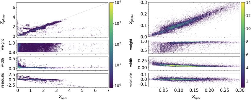
Z. Ansari et al.: Mixture models for photometric redshifts

Fig. 1. Spectroscopic data set in equatorial coordinates. Data are taken
from SDSS-DR15 + WISE totalling about 245 000 objects of which
there are 86 412 stars (yellow), 83 119 galaxies (purple) and 75 955
quasars (green). The entire photometric data set is a sample of about
1 023 000 objects, of which 98% lack spectroscopic redshifts and clas-
sification.

                                                                            Fig. 3. Redshift distribution of the spectroscopic data set. Top panel:
Fig. 2. Histogram showing i-band magnitudes of the objects from the         galaxies (purple) and quasars (green) in 0.1 redshift bins. Bottom panel:
photometric (blue) and spectroscopic data sets for stars (yellow), galax-   stars (yellow) in 0.0001 redshift bins.
ies (purple) and quasars (green), in 0.1 magnitude bins.

                                                                            2.2. Infinite Gaussian mixture models
their spectroscopic redshift (from the SDSS pipelines) smaller
than 1%. For only one MDN training, we added u-band PSF as                  In a Gaussian mixture model (GMM), the density distribution
well as model magnitudes. Our complete data sets are composed               of objects in ‘feature space’ (equivalent to photometric space,
of a photometric and a spectroscopic data set. For about 2% of              see Sect. 2.1) is described by a sum of Gaussian density compo-
the photometric data set we have spectroscopic information. This            nents. The GMM is a probabilistic model which requires that a
data set is called the ‘spectroscopic data set’. For the IGMM,              data set is drawn from a mixture of Gaussian density functions.
we have in total 1 022 731 unique sources from PhotoObjAll                  Each Gaussian distribution is called a component. As the Gaus-
and WISE, with additional 11 358 unique galaxies from WiggleZ               sian distributions are defined in all the dimensions of the feature
(Drinkwater et al. 2010) cross-matched with PhotoObjAll and                 space, they are characterised by a mean vector and a covariance
WISE. For the test samples, the spectroscopic data set contains             matrix. The feature vector contains the photometric information
86 412 unique stars, 83 119 unique galaxies and 75 955 quasars              of each astronomical source. To describe the GMM, whenever
from SpecPhoto and WISE according to the classification of                  needed, we use the notation πk N(x|µk , Σk ), where k(∈ {1, . . . , K})
their spectra by the SDSS pipelines (see Fig. 1).                           is the component index, µk , Σk and πk are the mean vector and the
    Figure 2 shows a general issue that is common to the litera-            covariance matrix in feature space, and the weight of component
ture on photo-zs, i.e., (by survey construction) the spectroscopic          k, respectively.
training sets do not reach the same depth as the photometric                     Since the GMM is a Bayesian method, it requires multi-
ones. This highlights the need for techniques that can extrapo-             ple sets of model parameters and hyperparameters. The model
late smoothly and with realistic uncertainties outside the ranges           parameters (means, covariances) change across the Gaussian
of a limited spectroscopic training set. Figure 3 shows the red-            components, while the hyperparameters are common to all of
shift distribution of different classes of objects from the spectro-        the Gaussian components, because they describe the priors from
scopic data set. Evidently, galaxies are mainly placed at redshifts         which all Gaussian components are drawn. For the GMM, the
.1, while quasars extend out to redshifts ∼7.                               number of Gaussian components is a fixed hyperparameter.
                                                                                                                                  A90, page 3 of 16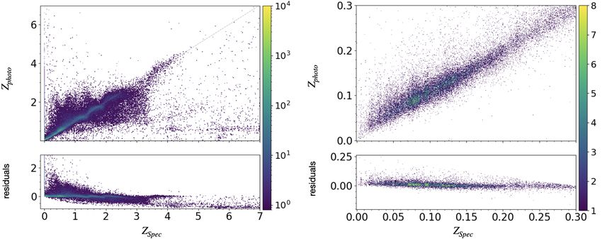
A&A 650, A90 (2021)

                                                                               Whenever needed, each object is assigned to the component
                                                                          to which its membership probability is maximal. In that case, we
                                                                          say that a component contains a data point.
                                                                               The IGMM provides different possible representations of the
                                                                          same data set for each set of hyperparameters: here, we are inter-
                                                                          ested in finding out the optimal number of components that can
                                                                          adequately describe the majority of the data. We then introduce
                                                                          a lower threshold on the number of sources that each component
                                                                          contains, and drop the components which contain less than the
                                                                          threshold. The threshold is defined by considering the size of the
                                                                          photometric sample and the highest value that we considered for
                                                                          the Dirichlet γ prior. The IGMM starts with components that con-
                                                                          tribute to 0.5% of the size of the photometric sample, since the
                                                                          highest γ value is 510 000 (see appendix for further details), due
Fig. 4. Maximum number of components vs. final number of compo-
                                                                          to our chosen ranges of hyperparameters. Therefore, we use 0.5%
nents for different IGMM realisations, restricted to Gaussian compo-      of the size of the photometric data set as the threshold. Figure 4
nents that contain at least 0.5% of the photometric data. Blue filled     shows that the final number of components converges to 48 ± 4.
circles represent IGMM realisations that needed more than 2000 iter-      The convergence indicates that the models do not need more than
ations to converge, while purple filled circles mark IGMM realisations    48 ± 4 components to describe the sample. Moreover, the initial
that needed less than 2000 iterations. The size of the symbols scales     1:1 ramp-up in the figure shows that the final number of compo-
with three different values of the prior of the Dirichlet concentration   nents is the same as the maximum tolerance, and so the model
(γ). The light blue shaded region represents the confidence interval of   cannot adequately describe the data set; this trend breaks at about
99% of regression estimation over the IGMM profiles by a multivariate     44 components. To guide the eye, we determine a regression sur-
smoothing procedure.                                                      face of all the IGMM profiles by a multivariate smoothing pro-
                                                                          cedure3 . In what follows, we choose 52 components.
                                                                               The first IGMM implementation was fully unsupervised, as
     The IGMM is the GMM case with an undefined number of                 it was optimised to only describe the distribution of the objects
components, which is optimised by the model itself, depend-               in feature space. Subsequently, we trained different IGMMs con-
ing on the photometric data set used. In particular, the IGMM             sidering additional spectroscopic information available for ≈2%
describes a mixture of Gaussian distributions on the data popu-           of the photometric sample. In particular, these partially super-
lation with an infinite (countable) number of components, using           vised implementations are trained using the entire photometric
a Dirichlet process (Teh 2010) to define a distribution on the            feature space including either (i) spectroscopic classifications or
component weights.                                                        (ii) spectroscopic redshifts or (iii) spectroscopic classifications
     However, setting an initial number of Gaussian density com-          and redshifts. Since the objects with additional spectroscopic
ponents is required by the IGMM. Based on the weights that                information are a small part of the photometric training sample
are given to each such component at the end of the model                  (≈2%), the implementations ensure that the SDSS spectroscopic
training, it is common practice to exclude the least weighted             preselection does not bias the IGMM over the entire photomet-
components and define the data population only by the highest-            ric sample. Finally, we calculate the membership probabilities to
weighted components. To pursue a fully Bayesian approach, it is           the 52 components for each object in the spectroscopic data set
advisable to explore a set of model hyperparameters with dif-             (≈2.45 × 10⁵ objects) from the optimised IGMM. This allows
ferent initial guesses for the number of components. Like its             us to assign each object from the spectroscopic sample to one
finite GMM counterpart, each realisation of IGMM estimates the            component. Thereafter, we label each of the IGMM components
membership probability of each data point to each component.              based on the percentage of spectroscopic classes that it contains.
Appendix B provides a summary of the IGMM formalism.                           Figure 5 shows the population of objects from the spectro-
     For this work, we used the built-in variational IGMM pack-           scopic data set and their corresponding IGMM components in
age from the scikit-learn library for our implementations.                g − r vs. z − w1 (upper panel) and w2 vs. w1 − w2 (bottom panel)
In practice, the variational optimiser uses a truncated distri-           colour-colour and colour-magnitude diagrams. Each row from
bution over component weights with a fixed maximum num-                   left to right shows the assigned components to stars, galaxies
ber of components, known as stick-breaking representation                 and quasars in the respective panels.
(Ferguson 1973), with an expectation-maximisation algorithm
(Dempster et al. 1977). To optimise the model and find the best           2.3. Mixture density networks
representation of the data set, we explored a range of param-
eters. We increased the maximum number of allowed Gaus-                   MDNs are a form of ANNs, which are capable of arbitrarily
sian components from 10 to 100 in increments of 2 and we set              accurate approximation to a function and its derivatives based
the maximum number of iterations for expectation maximisa-                on the Universal Approximation Theorem (Hornik 1991). ANNs
tion performance to 2000. We used a Dirichlet concentration (γ)           can be used for regression or classification purposes. ANNs are
of each Gaussian component (k) on the weight distribution, of             structured in layers of neurons, where each neuron receives an
either 0.01, 0.05 or 0.0001 times the number of objects in the            input vector from the previous layer, and outputs a nonlinear
training data set. The covariance matrix for each Gaussian com-           function of it that is passed on to the next layer. In MDNs, the
ponent was defined as type ‘full’; as per definition, each com-           aim is to approximate a distribution in the product space of input
ponent has its own general covariance matrix. Furthermore, the            vectors of the individual sources ( f i ) and target values (e.g.,
prior on the mean distribution for each Gaussian component is
defined as the median of the entries of the input vectors of the          3
                                                                            https://has2k1.github.io/scikit-misc/stable/
training data set (i.e., magnitudes, extinction).                         generated/skmisc.loess.loess.html

A90, page 4 of 16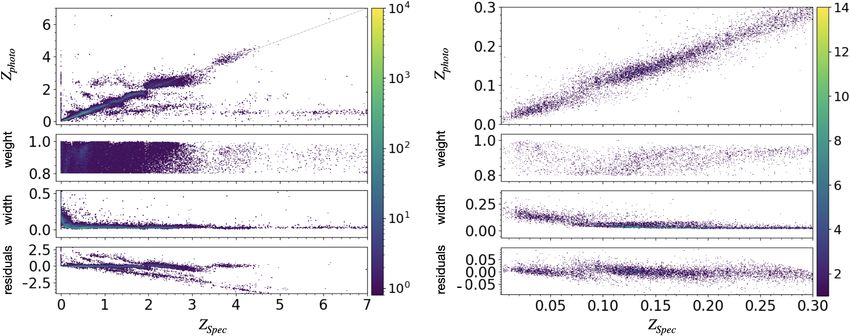
Z. Ansari et al.: Mixture models for photometric redshifts
Fig. 5. Colour-colour and colour-magnitude diagrams. Shown are g − r vs. z − W1 colour-colour diagrams (upper panel) and W2 vs. W1 − W2
colour-magnitude diagrams (bottom panel) for a populations of objects from the spectroscopic data set such as stars (left column), galaxies (middle
column) and quasars (right column). The purple contours correspond to the 68th percentile of each Gaussian IGMM component. The green filled
circles correspond to the means µk of the Gaussian components. The grey scale indicates the abundance of the sources in each diagram.
z s,i ) as a superposition of different components. MDNs (Bishop photometric features (see Sect. 2.1) along with the membership
1994) are trained to optimise the log-likelihood probabilities of the IGMM, which carry additional information
N of the object classes (stars, galaxies and quasars). The dimen-
N c
X X sion of the MDN input space is 74, of which 52 are the IGMM
log L = log p̂k ( f i )N(z s,i |mk ( f i ), sk ( f i )) (1) membership probabilities and 22 are the feature-space entries.
i=1 k=1 The output layer of the MDN is defined by three neurons for
by approximating the averages mk ( f ), amplitudes p̂k ( f ) and each branch: the average redshift on the branch, the width of
widths sk ( f ). Here, N is the number of objects in the spectro- the branch and the membership probability of the source to the
scopic data set, while Nc denotes the number of output compo- branch. The MDN is fully connected, that is the neurons in one
nents (or branches) of the MDN. layer are connected to all of the neurons in the next layer. Due
Due to the limited information provided by the photometric to the fact that the MDN input contains the IGMM member-
space, a source of a specific spectroscopic class and low red- ship probabilities, after MDN hyperparameter optimisation, we
shift can be confused with a different spectroscopic class and train one MDN for each of the four IGMM implementations as
high redshift. Therefore, by providing distributions over a full described in previous sections.
range of redshifts, MDNs can cope with the fact that colours We randomly split the entire spectroscopic data set Sect. 2.1
are not necessarily monotonic with redshift (as is the case e.g., and use 80% for training and 20% for validation of the MDN. In
in quasars). In order to avoid confusing MDN components with order to optimise the MDN, we explored neural networks with 0
IGMM components, here we call MDN components branches. to 3 hidden layers. Each layer with a discrete number of neurons
For the sake of reproducibility, we use a publicly available in the interval [3, 7, 10, 74, 100, 156, 222, 300, 400, 500, 528,
MDN wrapper around the keras ANN module4 and a sim- 600, 740]. Furthermore, we used a discrete number of branches
ple MDN architecture. The MDN input layer contains the same for the MDN in the interval [10, 52, 56, 100, 300]. The stan-
dard rectified linear unit (ReLU, Nair & Hinton 2010) and para-
4 metric rectified linear unit (PReLU, He et al. 2015) are used as
https://github.com/cpmpercussion/keras-mdn-layer
A90, page 5 of 16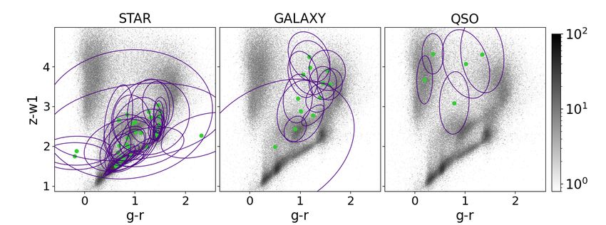
A&A 650, A90 (2021)

                                                                        3. Results
                                                                        We trained an IGMM on the photometric data set (see Sect. 2.1),
                                                                        using the optimal hyperparameters (Sect. 2.2). Thereafter, we
                                                                        linked IGMM components to the three spectroscopic classes
                                                                        using a spectroscopic data set (Sect. 2.1). Finally, we imple-
                                                                        mented MDNs on the spectroscopic data set using photomet-
                                                                        ric features and membership probabilities from the IGMM
                                                                        to estimate the conditional probability distribution p(z p | f ) of
                                                                        photo-z values from the photometric inputs. In this section, we
                                                                        describe the evaluation methods and the resulting classification
                                                                        and photo-z estimations.

                                                                        3.1. Classification
                                                                        With our mixture models we address the common problem
                                                                        of cross contamination among different classes of objects due
Fig. 6. MDN Loss (− log(L)/N) as a function of epoch. The loss          to the a priori unknown underlying spectral energy distri-
obtained during the MDN training and validation are shown by blue       bution. In the IGMM realisations, each object can belong
and orange lines, respectively.                                         to each of theP components with a probability pi,k =
                                                                        wk N( f i |µk , Σk )/ l (wl N( f i |µl , Σl )), which we denote by mem-
                                                                        bership probabilities in the following. As we introduced above
                                                                        (end of Sect. 2.2), the simplest way to assign an object (with
                                                                        feature vector f i ) to a component is to consider the component
                                                                        index k̂ for which pi,k̂ is maximised.
                                                                            To parameterise the accuracy of the classification, we con-
                                                                        sider the usual quantification of true and false positives and true
                                                                        and false negatives (e.g., Fawcett 2006), and build a confusion
                                                                        matrix to quantify the rate of correct classifications. Figure 7
                                                                        shows the confusion matrix of the GMM-based classification
                                                                        for the spectroscopic data set. The true positive rates5 for stars,
                                                                        galaxies and quasars are 0.97, 0.91 and 0.95, respectively. False
                                                                        positive rates for stars that are true galaxies and quasars are
                                                                        0.0029 and 0.029. False negative rates for stars that are assigned
                                                                        to galaxies and quasars are 0.031 and 0.019 of all stars, respec-
                                                                        tively. The accuracy6 is ≈94%. This means that the IGMM part
                                                                        of our mixture models can clean an extragalactic sample from
                                                                        most of stellar contaminants, and broadly separate galaxies from
                                                                        AGN-dominated objects. We compare the performance of our
                                                                        classification to that of a HDBSCAN classification (Campello et al.
                                                                        2013) of a subset of 39 447 objects from the SDSS-DR14 that
                                                                        have an accuracy of ≈95% using ugrizY HJKw1w2-band mag-
Fig. 7. IGMM confusion matrix. The spectroscopic classifications are    nitudes (Logan & Fotopoulou 2020). We find that our method
shown against the IGMM classes of the spectroscopic data set.           achieves a comparable accuracy even without u-band and
                                                                        Y JHK-band magnitudes.
                                                                            Figure 5 demonstrates that the IGMM recognises the main
                                                                        behaviours of stars, galaxies and quasars in colour space and
activation functions. We used ADAM as optimiser and batch learn-        also identifies subclasses that are not highly represented in the
ing with 64 objects per epoch with learning rates of 10−6 , 10−5 ,      spectroscopic sample, such as white dwarfs and brown dwarfs.
10−4 and 10−3 to mitigate local minima of the loss function.            On the other hand, some components happen to lie in regions
    By comparing the training and validation loss of MDNs with          of the colour-magnitude-extinction space that are not domi-
the previously defined set of hyperparameters, the resulting opti-      nated by only one subclass. The overlap between different object
mal set of hyperparameters contains a hidden layer with 528 neu-        classes in photometry can affect the classification performance
rons and 10 MDN branches. The activation function is PReLU              and the output of the classification that is then used by the MDN
and the learning rate for the ADAM optimiser is 10−4 . Figure 6         regression. The components corresponding to regions of overlap
shows the loss function, − log(L)/N, for the training and val-          between different classes are discussed below.
idation data set, for the MDN optimisation for which mem-                   Approximately 30% of IGMM components that cover ≈15%
bership probabilities are obtained from the partially supervised        of the spectroscopic data set, marked in red in Table 1, con-
IGMM realisation that also considers the spectroscopic classes.         tain a non-negligible fraction of objects from more than one
As Fig. 6 shows, the learning curve flattens roughly around 300         of the three main classes. Figure 8 shows their position in the
epochs. To mitigate overfitting, we concluded that 300 epochs
are sufficient to train the model. Additionally to training MDNs
with the redshifts as targets, we tested log(z s ) as a target and it   5
                                                                            Defined as: TP/(TP+FN).
                                                                        6
led to an improvement in the z p estimation.                                Defined as: (TP+TN)/(TP+TN+FN+FP).

A90, page 6 of 16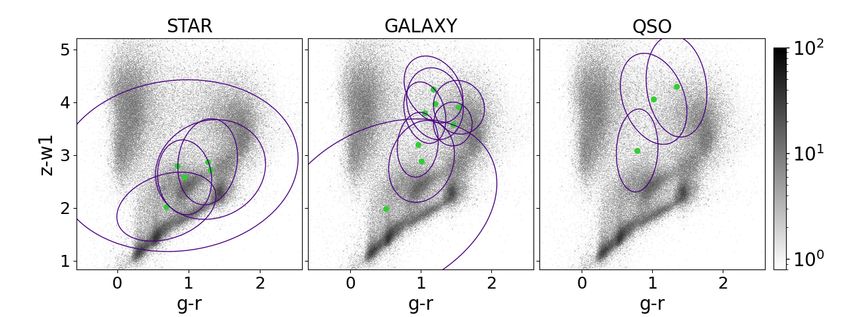
Z. Ansari et al.: Mixture models for photometric redshifts

Table 1. Percentage of objects from each spectroscopic class (stars,       same colour-colour and colour-magnitude diagrams as Fig. 5.
galaxies, quasars) within each IGMM component.                             We address these components as ‘problematic components’.
                                                                               As expected, the problematic components lie at the faint
      IGMM       Stars                Galaxies       Quasars               end (with higher magnitude uncertainties in WISE), or in inter-
      components                                                           mediate regions of the colour space between AGN-dominated
                                                                           and galaxy-dominated systems. Additionally, the SDSS spec-
      1               85.42           0.27           14.31                 troscopic classification of some objects is ambiguous and for
      2               99.98           0              0.02                  some cases the automatic classification (by the SDSS spec-
      3               97.46           0.06           2.48                  tral pipelines) is either erroneous or has multiple incompatible
      4               100             0              0                     entries7 . These issues occur more frequent for fainter objects
      5               1.57            0.54           97.88                 which have spectra with low signal-to-noise ratio8 . However,
      6               99.86           0.05           0.1                   since most of the objects are clustered in three main classes
      7               3.7             86.06          10.24                 which are correctly identified by the IGMM components, uncer-
      8               100             0              0                     tain spectroscopic labels are not a significant problem for our
      9               97.45           0.05           2.5                   calculations.
      10              8.94            71.67          19.39
      11              1.97            90.16          7.87
      12              6.95            52.25          40.80                 3.2. Photometric redshifts
      13              99.6            0              0.4                   Here we discuss different metrics employed to evaluate the per-
      14              100             0              0                     formance of our methods used to determine photometric red-
      15              42.38           43.22          14.41                 shifts. Most metrics are based on commonly used statistical
      16              55.39           0.43           44.18                 methods as outlined. The prediction bias is defined as the mean
      17              99.93           0.01           0.06                  of weighted residuals, ∆z = (z p − z s )/(1 + z s ), which is the same
      18              96.75           2.48           0.77                  as the definition in Cohen et al. (2000). The root-mean-square of
      19              6.58            36.44          56.98                 the weighted residuals is defined as rms(∆z). The fraction of out-
      20              99.89           0              0.11                  liers is defined as the number of objects with 3 × rms(∆z) < ∆z.
      21              1.14            94.51          4.35                      For all methods, we excluded objects with spectroscopic red-
      22              98.02           0.07           1.90                  shift errors δz s > 0.01 × (1 + z s ). For each source, the MDN deter-
      23              99.94           0              0.06                  mines a full photo-z distribution, which is a superposition of all
      24              3.69            89.54          6.77                  branches, each with a membership probability, average, and dis-
      25              100             0              0                     persion. If one so-called point estimate is needed, there are at least
      26              99.94           0.01           0.05                  two options to compute it. One option is the expectation value
      27              97.48           0.47           2.05
      28              100             0              0
                                                                                            P
                                                                                               µk ( f ) p̂k
      29              12.31           20.04          67.65                 E(z p,i | f i ) = k P i ,                                           (2)
                                                                                                k p̂k
      30              100             0              0
      31              1.02            96.60          2.38                  weighted across all branches that an object can belong to,
      32              11.13           35.58          53.28                 according to its branch membership probabilities. Another
      33              99.96           0.02           0.02                  choice, which we follow here, is the peak µr ( f i ) of the branch
      34              99.71           0              0.29                  that gives the maximum membership probability of a given
      35              100             0              0                     object. In what follows, we refer to this redshift value as the
      36              99.8            0.1            0.1                   ‘peak photo-z’.
      37              34.23           42.05          23.72                     In a fully Bayesian framework, one would also consider the
      38              100             0              0                     maximum-a-posteriori, which in our approach would correspond
      39              8.43            51.74          39.83                 with the photo-z that maximises the MDN output sum of Gaus-
                                                                           sians because all our priors are uniform. Strictly speaking, in
      40              99.91           0              0.09
                                                                           principle the maximum-a-posteriori and the peak redshift are not
      41              99.51           0.04           0.45
                                                                           the same, if the MDN Gaussian with the highest membership
      42              100             0              0                     probability lies close to other MDN Gaussians. Here, for the sake
      43              4.43            88.61          6.97                  of computational convenience we choose the peak redshift, leav-
      44              0.56            98.18          1.25                  ing the comparison with other possible choices (including the
      45              90.3            0.83           8.87                  maximum-a-posteriori, or non-uniform priors) to future inves-
      46              79.57           1.22           19.21                 tigation. We also note that this distinction becomes important
      47              2.87            65.41          31.72                 for objects whose membership probabilities are not clearly dom-
      48              0.73            0.05           99.21                 inated by one of the MDN output Gaussians. In the follow-
      49              100             0              0                     ing, we examine the photo-z estimation performance on objects
      50              60.24           0.74           39.02                 whose membership probabilities to one of the MDN Gaussians
      51              44.52           26.33          29.15                 is >80%, in which case there is almost no difference between
      52              95.64           0.04           4.32                  peak redshit and maximum-a-posteriori redshift.
Notes. The components highlighted in red lie between different spec-
                                                                           7
troscopic class regions in photometric feature space, and can reduce the       For example for OBJID=1691188859137714176 from SDSS-DR15.
                                                                           8
classification accuracy.                                                       For example for OBJID=743142903307593728 from SDSS-DR15.

                                                                                                                                A90, page 7 of 16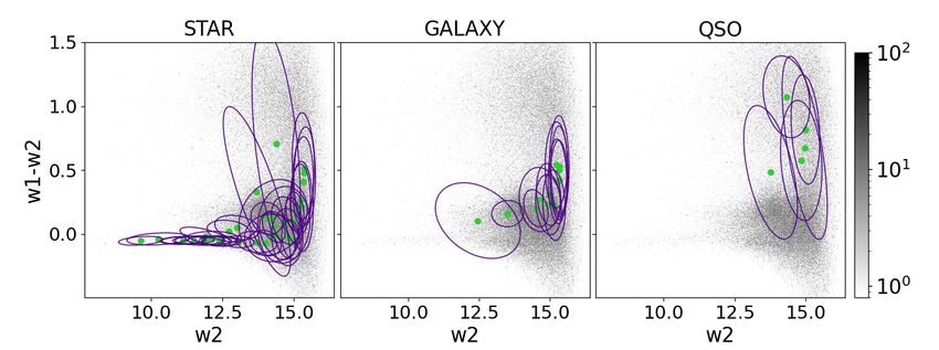
A&A 650, A90 (2021)
Fig. 8. Colour-colour and colour-magnitude diagrams. Shown are g−r vs. z−W1 colour-colour diagrams (upper panel) and W2 vs. W1−W2 colour-
magnitude diagrams (bottom panel) for objects from the spectroscopic data set of the three spectroscopic classes such as stars (left column), galaxies
(middle column) and quasars (right column). The purple contours correspond to the 68-th percentile of the problematic Gaussian components of the
IGMM that are not dominated by objects of just one spectroscopic class. The green filled circles correspond to the means µk of these components.
The grey scale indicates the number of sources in each diagram.
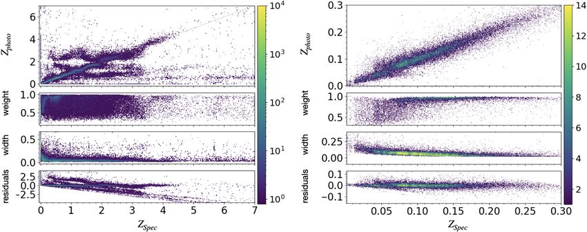
Figure 9 shows the distribution of peak photo-zs (top) and object belongs to a branch. As demonstrated in Fig. 10, bot-
expectation photo-zs (bottom) versus spectroscopic redshifts, z s , tom panel, the MDN performs indeed better for objects with
for the MDN run with ten branches. One aspect to consider increased confidence level.
when determining photo-z in cosmological wide-field imag-
ing surveys, is the availability of u-band magnitudes, which
is currently available for KiDS but not for DES. The Rubin 4. Conclusion
LSST is expected to deliver u-band photometry at the same Performance evaluations of MDN photo-zs from different
depth of KiDS over ≈12 300deg2 (Y1) and ≈14 300deg2 (Y2) IGMM realisations are summarised in Table 2. The minimum
(The LSST Dark Energy Science Collaboration 2018). To test MDN photo-z bias and rms of different IGMM realisations with-
the effect, we re-trained one of our mixture models (IGMM spec. out using u-band magnitudes is reached by the IGMM realisation
class) for a data set that includes u-band PSF and model magni- (Spec. class, (z s )) that uses the spectroscopic classifications and
tudes as additional input features (Fig. 10). The bias and root- spectroscopic redshifts of ≈2% of the dataset. This implies that
mean-square residuals are provided in Table 2 for all objects and the IGMM can provide a reasonable description of the objects
for galaxies with spectroscopic redshifts z s < 0.3, z s < 0.4, and in their feature space even with very limited spectroscopic infor-
z s < 0.5. This test leads to a lower rms ∆z and smaller fraction mation. On the other hand, for this realisation the fraction of 3σ
of 3σ outliers than for the same model without u-band magni- outliers is not as low as for other IGMM realisations (Tables 2
tudes and can be considered an improvement in accuracy. One and 3) which have a slightly higher bias and rms. For the valida-
reason is that for low redshift objects, u-band contains informa- tion samples that are restricted to galaxies with a spectroscopic
tion on the position and strength of the 4000 Å Balmer-break, redshift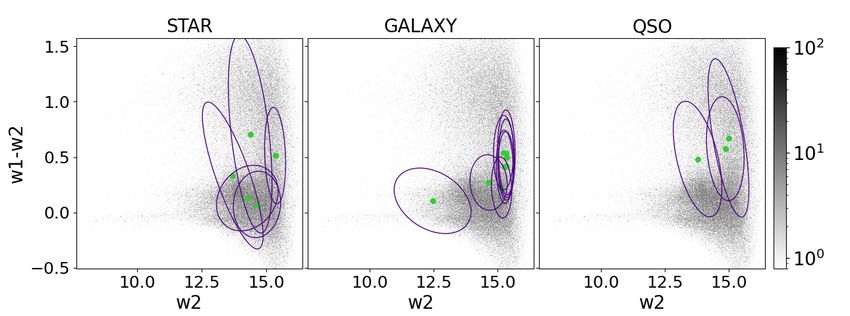
Z. Ansari et al.: Mixture models for photometric redshifts

Fig. 9. Comparison of spectroscopic vs. MDN photometric redshifts. The photometric redshifts are taken from the partially supervised ‘spec. class’
IGMM implementation (as described in Sect. 2.2). The colour-scales indicate the number of objects. Top panels: predicted photometric redshifts
that correspond to the branches with the highest weights. The single panels show the weights, dispersions (denoted by ‘width’) and residuals from
top to bottom. Bottom panels: mean photometric redshifts of the predicted redshifts over all branches with respect to their weights. Lower panel:
residuals. Left panels: include all classes with zspec < 7. Right panels: include all galaxies with zspec < 0.3.

confidence (i.e., weightmax > 0.8) is summarised in Table 3. In           a fifth of the SDSS photo-z sample. As summarised in Table 4
order to compare our photo-z estimates to those from the SDSS,            and shown in Fig. 11, our method improves the bias of photo-z
we select objects from the SDSS SpecObjAll table that have                estimates by about one order of magnitude compared to SDSS
photo-zs (obtained with a kNN interpolation) from the SDSS                photo-zs for objects for which our model estimated the photo-
PhotoObjAll (38 487 objects). We remark that our MDN yields               zs at high confidence (i.e., weightmax > 0.8), and our method
the full photo-z PDF, so a choice must be made when compar-               also decreases the rms and the fraction of outliers. All metrics
ing its results with point estimates from other methods in the            are improved, with the added advantage that the MDN computes
literature. For this reason, we follow our previous choice and            photo-zs for all objects (instead of just those with low stellar-
consider the peak photo-z’s. We compare our photo-z’s to the              ity) and can also cover the z s > 1 range more accurately than
SDSS ones for the full sample (38 487 objects) and also for the           the SDSS kNN. As a matter of fact, the SDSS photo-zs hardly
subset of objects that belong to a MDN branch with high confi-            exceed z p ≈ 1, while our machinery is trained over a much wider
dence (weightmax > 0.8, 18 355 objects). To account for uncer-            redshift range.
tainties in bias and rms due to the finite sample size, we split               As a general benchmark, the LSST system science require-
the whole sample into five sub-sets, compute the bias and rms             ments document9 defines three photometric redshift require-
on each, and then report their average and standard deviation.            ments for a sample of four billion galaxies with i < 25 mag
As an alternative, we also evaluate the bias, rms and fraction of         within z s < 0.3 as follows: First, for the error in (1+z s ) the rms of
outliers when the MDN is trained with a k-fold cross-validation
                                                                          9
method (see e.g Altman & Bland 2005) on the full SDSS train-                https://docushare.lsstcorp.org/docushare/dsweb/Get/
ing set (≈245 000 objects), where each of the k = 5 folds exclude         LPM-17

                                                                                                                               A90, page 9 of 16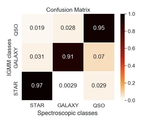
A&A 650, A90 (2021)

Fig. 10. Photo-z performance of different MDN implementations. Top panel: retaining only objects with weightmax > 0.8 membership probability to
a MDN branch. Middle panel: including u-band PSF and model magnitudes. Bottom panel: u-band magnitudes and MDN branch weightmax > 0.8.
Left column: all types of objects in the spectroscopic data set. Right column: only galaxies in z s < 0.3. from the spectroscopic data set.

residuals is lower than 0.02. Secondly, the fraction of 3σ (‘catas-      samples from the SDSS do not reach as deep as the Rubin
trophic’) outliers is lower than 10% of the sample and thirdly, the      LSST is expected to, our method shows promising results as
bias is lower than 0.003.                                                a starting point. A general remark, which holds for all photo-
     In our approach, these requirements are met if the MDN              z estimation methods is that a re-training for the LSST regime
peak z p is adopted. The rms ∆z can be brought to 0.02 over 0 <          may also need deeper photometric and more robust spectro-
z s < 0.5 both for all objects (Table 5) and for ‘high-confidence’       scopic samples. Recently, Beck et al. (2021) used neural net-
objects with >0.8 membership probability to a branch (Table 6;           works to classify objects in the Pan-STARRS1 footprint, which
called weight in Sect. 2.3). Although our training and evaluation        is known to have a more accurate photometry than the SDSS

A90, page 10 of 16
Z. Ansari et al.: Mixture models for photometric redshifts
Table 2. MDN performance evaluation, without any clipping for the average and rms, without any threshold on branch membership probabilities.
IGMM Photometry h∆zi rms(∆z) 3σ outliers h∆zi, rms(∆z), 3σ outliers, rms(∆z), rms(∆z),
implementation (all) (all) (all) range1 (a) range1 (a) range1 (a) range2 (b) range3 (c)
Fully unsup. griz, W1, W2 0.0152 0.2174 3.08% 0.0007 0.0177 0.28% 0.0988 0.0945
Spec. class griz, W1, W2 0.0111 0.2069 1.31% 0.0006 0.0167 0.41% 0.0822 0.0783
Spec. class (d) griz, W1, W2 0.0356 0.2300 1.35% 0.0110 0.0260 0.71% 0.0953 0.0903
Redshift (z s ) griz, W1, W2 0.0176 0.2131 3.21% −0.0009 0.0174 0.38% 0.0896 0.0873
Spec. class, z s griz, W1, W2 0.0047 0.1990 2.66% 0.0036 0.0181 0.57% 0.0675 0.0664
Spec. class ugriz, W1, W2 0.0135 0.1592 1.62% 0.0007 0.0160 0.23% 0.0601 0.0611
Notes. Spectroscopic sample for all IGMM implementations containing stars, galaxies and quasars. (a) Restricted to galaxies with z s < 0.3;
restricted to galaxies with z s < 0.4; (c) restricted to galaxies with z s < 0.5; (d) expectation value. Fully unsup.: Fully unsupervised IGMM imple-
(b)
mentation. Spec. class: uses spectroscopically classified objects (e.g., stars, galaxies, and quasars) for those which SDSS provides spectroscopic
information (i.e., ≈2% of the photometric data set) to classify the data. Redshift (z s ): uses the spectroscopic redshift of objects from ≈2% of the
photometric data set to classify the data. Spec. class, (z s ): uses both, spectroscopically classified objects and the spectrsocopic redshift of objects
from ≈2% of the photometric data set to classify the data.
Table 3. MDN performance evaluation exclusively for sources with MDN branch weightmax > 0.8, without any clipping for the average and rms.
IGMM Photometry h∆zi rms(∆z) 3σ outliers h∆zi, rms(∆z), 3σ outliers, rms(∆z), rms(∆z),
implementation (all) (all) (all) range1 (a) range1 (a) range1 (a) range2 (b) range3 (c)
Fully unsup. griz, W1, W2 0.0032 0.1165 1.00% 0.0007 0.0177 0.60% 0.0350 0.0360
Spec. class griz, W1, W2 0.0031 0.1244 0.93% 0.0006 0.0167 0.83% 0.0405 0.0391
Redshift (z s ) griz, W1, W2 0.0035 0.1076 0.79% −0.0009 0.0174 0.52% 0.0299 0.0331
Spec. class, z s griz, W1, W2 −0.0048 0.1170 1.02% 0.0036 0.0036 1.02% 0.0337 0.0314
Spec. class ugriz, W1, W2 0.0043 0.0934 0.66% 0.0007 0.0160 0.92% 0.0334 0.0341
Notes. (a) Restricted to galaxies with z s < 0.3; (b) restricted to galaxies with z s < 0.4; (c) restricted to galaxies with z s < 0.5. The IGMM implemen-
tation abbreviations are the same as for Table 2.
Table 4. Comparison between the photo-z evaluation on all objects from the spectroscopic sample with available SDSS photo-zs.
No k-fold in MDN; IGMM Restriction on Number of Bias rms 3σ outliers
implementation objects objects
SDSS griz photo-z None 38 632 0.0001 ± 0.0008 0.0458 ± 0.0483 (0.73 ± 0.22)%
MDN spec. class + griz, W1, W2 None 38 632 0.0018 ± 0.0014 0.0478 ± 0.0384 (0.49 ± 0.04)%
SDSS griz photo-z weightmax > 0.8 18 355 −0.0038 ± 0.0040 0.0394 ± 0.0413 (0.46 ± 0.19)%
MDN spec. class + griz, W1, W2 weightmax > 0.8 18 355 −0.0002 ± 0.0009 0.0389 ± 0.0318 (0.55 ± 0.26)%
k-fold in MDN; IGMM Restriction on Number of Bias rms 3σ outliers
implementation objects objects
SDSS griz photo-z None 38 632 0.0001 ± 0.0020 0.0662 ± 0.0072 (0.79 ± 0.22)%
MDN spec. class + griz, W1, W2 None 38 632 0.0027 ± 0.0031 0.0724 ± 0.0139 (0.45 ± 0.10) %
SDSS griz photo-z weightmax > 0.8 23 908 −0.0028 ± 0.0029 0.0506 ± 0.0096 (0.33 ± 0.14)%
MDN spec. class + griz, W1, W2 weightmax > 0.8 23 908 0.00011 ± 0.0042 0.0458 ± 0.0069 (0.28 ± 0.07)%
Table 5. MDN performance evaluation.
IGMM implementation Photometry h∆zi (z s < 1) rms(∆z) (z s < 1) h∆zi, range1 (a)
Fully unsup. griz, W1, W2 0.0007 ± 0.0006 0.0204 ± 0.0106 0.0025 ± 0.0005
Spec. class griz, W1, W2 0.0030 ± 0.0028 0.0216 ± 0.0104 0.0042 ± 0.039
Redshift (z s ) griz, W1, W2 0.0022 ± 0.0024 0.0207 ± 0.0113 0.0008 ± 0.0003
Spec. class, z s griz, W1, W2 0.0001 ± 0.0005 0.0208 ± 0.0112 0.0058 ± 0.0006
Spec. class ugriz, W1, W2 0.0023 ± 0.0026 0.0181 ± 0.0091 0.0004 ± 0.0025
IGMM implementation photometry rms(∆z), range1 (a) rms(∆z), range2 (b) rms(∆z), range3 (c)
Fully unsup. griz, W1, W2 0.0215 ± 0.0013 0.0233 ± 0.0013 0.0238 ± 0.0015
Spec. class griz, W1, W2 0.0230 ± 0.0015 0.0245 ± 0.0019 0.0247 ± 0.0014
Redshift (z s ) griz, W1, W2 0.0219 ± 0.0014 0.0238 ± 0.0012 0.0242 ± 0.0013
Spec. class, z s griz, W1, W2 0.0218 ± 0.0019 0.0235 ± 0.0019 0.0235 ± 0.0024
Spec. class ugriz, W1, W2 0.0179 ± 0.0015 0.0182 ± 0.0016 0.0187 ± 0.0019
Notes. The bias and rms are computed using the definition of clipped bias and rms in PS1-STR (Beck et al. 2021). (a) Restricted to galaxies with
z s < 0.3; (b) restricted to galaxies with z s < 0.4; (c) restricted to galaxies with z s < 0.5.
A90, page 11 of 16A&A 650, A90 (2021)
Table 6. MDN performance evaluation exclusively for sources with MDN branch weightmax > 0.8.
IGMM implementation Photometry h∆zi (z s < 1) rms(∆z) (z s < 1) h∆zi, range1 (a)
Fully unsup. griz, W1, W2 0.0004 ± 0.0010 0.0249 ± 0.0038 0.0014 ± 0.0005
Spec. class griz, W1, W2 0.0035 ± 0.0030 0.0273 ± 0.0045 0.0015 ± 0.0009
Redshift (z s ) griz, W1, W2 0.0018 ± 0.0013 0.0236 ± 0.0045 −0.0004 ± 0.0004
Spec. class, z s griz, W1, W2 −0.0014 ± 0.0012 0.0264 ± 0.0054 0.0042 ± 0.0005
Spec. class ugriz, W1, W2 0.0036 ± 0.0026 0.0227 ± 0.0058 0.0009 ± 0.0005
IGMM implementation photometry rms(∆z), range1 (a) rms(∆z), range2 (b) rms(∆z), range3 (c)
Fully unsup. griz, W1, W2 0.0186 ± 0.0002 0.0201 ± 0.0003 0.0207 ± 0.0004
Spec. class griz, W1, W2 0.0181 ± 0.0002 0.0207 ± 0.0009 0.0214 ± 0.0007
Redshift (z s ) griz, W1, W2 0.0182 ± 0.0004 0.0195 ± 0.0005 0.0203 ± 0.0004
Spec. class, z s griz, W1, W2 0.0189 ± 0.0013 0.0205 ± 0.0014 0.0207 ± 0.0014
Spec. class ugriz, W1, W2 0.0163 ± 0.0007 0.0167 ± 0.0008 0.0170 ± 0.0010
Notes. The bias and rms are computed using the definition of clipped bias and rms in PS1-STR (Beck et al. 2021). (a) Restricted to galaxies with
z s < 0.3; (b) restricted to galaxies with z s < 0.4; (c) restricted to galaxies with z s < 0.5.
(Magnier et al. 2013), and evaluated photo-zs on objects with a
probability p > 0.8 of being galaxies, obtaining rms(∆z) = 0.03
over 0 < z s < 1. If we follow the same definitions and clip-
ping10 as by Beck et al. (2021), then we obtain 1.7–2% relative
rms over the 0 < z s < 0.5 redshift range. Our code for re-training
and any further evaluation is publicly accessible11 .
5. Discussion
Adding u-band information, as is the case with the SDSS and
will be the case with the LSST, reduces the bias and fraction of
outliers in all the redshift ranges considered. This is also because
adding u-band magnitudes sharpens the MDN separation into
branches and increases the fraction of objects with the highest
weighted branch >0.8, as can be seen in the bottom panels of
Fig. 9.
We remark that throughout this work, we are simply adopting
reddening values in the i-band (Ai ), which the SDSS provides via
a simple conversion of measured E(B − V) values with a Milky-
Way extinction law and RV = 3.1. Our approach accounts for
the systematic uncertainties due to the unknown extinction law
by producing probability distributions and associate uncertain-
ties for each photo-z value.
The combined information across the optical and infrared,
through the SDSS and WISE magnitudes, helps reducing the
overlap between different classes in colour-magnitude space.
The WISE depth is not a major limiting factor in the sample
completeness as long as samples from the SDSS are considered,
but it can affect the completeness significantly for deeper surveys
(Spiniello & Agnello 2019). In view of performing the classi-
fication and photo-z estimation on the DES, and on the Rubin Fig. 11. Top panel: SDSS spectroscopic redshift vs. SDSS photometric
LSST later on, deeper mid-IR data are needed. The unWISE redshift. Bottom panel: spectroscopic redshift vs. photometric redshift
reprocessing of the WISE cutouts improved upon the original (this work). Colour bars indicate the number of sources in the diagrams.
WISE depth (Lang 2014). Further in the future, forced photom- The selection of sources is made by retaining objects with weightmax >
0.8 membership probability to a MDN branch.
etry of the unWISE cutouts from wide-field optical and NIR
surveys may further increase the mid-IR survey depth (e.g.,
Lang & Hogg 2014).
In general, separating objects into many sub-classes aids the a subset of objects with more homogeneous properties than the
photo-z regression, as each MDN branch only needs to consider whole photometric sample. Furthermore, the approach that we
used in this work is both in the realm of machine learning (hence
10
Their clipping procedure removes objects with |∆z| > 0.15. less constrained by choices of templates) while it can also pro-
11
github.com/ZoeAnsari/MixtureModelsForPhotometric duce a full output distribution for the photo-z given the available
Redshifts photometric information. Beyond their first implementation in
A90, page 12 of 16Z. Ansari et al.: Mixture models for photometric redshifts
this work, mixture models can be easily adapted so that they can Driver, S. P., Hill, D. T., Kelvin, L. S., et al. 2011, MNRAS, 413, 971
account for missing entries and limited depth, as in the GMM Fawcett, T. 2006, Pattern Recognit. Lett., 27, 861
implementation by Melchior & Goulding (2018). Ferguson, T. S. 1973, Ann. Statist., 1, 209
Fernández-Soto, A., Lanzetta, K. M., & Yahil, A. 1999, ApJ, 513, 34
Galametz, A., Saglia, R., Paltani, S., et al. 2017, A&A, 598, A20
Acknowledgements. This work is supported by a VILLUM FONDEN Inves- Garilli, B., Le Fèvre, O., Guzzo, L., et al. 2008, A&A, 486, 683
tigator grant (project number 16599), a VILLUM FONDEN Young Investor Gerdes, D. W., Sypniewski, A. J., McKay, T. A., et al. 2010, ApJ, 715, 823
Grant (project number 25501), and a Villum Experiment Grant (project number Görür, D., & Edward Rasmussen, C. 2010, J. Comp. Sci. Technol., 25, 653
36225). This project is partially funded by the Danish council for indepen- Graham, M. L., Connolly, A. J., Ivezić, Ž., et al. 2018, AJ, 155, 1
dent research under the project “Fundamentals of Dark Matter Structures”, Guzzo, L., Scodeggio, M., Garilli, B., et al. 2014, A&A, 566, A108
DFF–6108-00570. He, K., Zhang, X., Ren, S., & Sun, J. 2015, ArXiv eprints [arXiv:1502.01852]
Hildebrandt, H., Köhlinger, F., van den Busch, J. L., et al. 2020, A&A, 633, A69
Hornik, K. 1991, Neural Networks, 4, 251
References Hoyle, B., Gruen, D., Bernstein, G. M., et al. 2018, MNRAS, 478, 592
Ilbert, O., Arnouts, S., McCracken, H. J., et al. 2006, A&A, 457, 841
Abbott, T. M. C., Abdalla, F. B., Allam, S., et al. 2018, ApJS, 239, 18 Joudaki, S., Blake, C., Johnson, A., et al. 2018, MNRAS, 474, 4894
Aguado, D. S., Ahumada, R., Almeida, A., et al. 2019, ApJS, 240, 23 Knox, L., Song, Y.-S., & Zhan, H. 2006, ApJ, 652, 857
Ahn, C. P., Alexandroff, R., Allende Prieto, C., et al. 2012, ApJS, 203, 21 Lang, D. 2014, AJ, 147, 108
Almosallam, I. A., Lindsay, S. N., Jarvis, M. J., et al. 2016, MNRAS, 455, 2387 Lang, D., & Hogg, D. W. 2014, ApJ, 151, 36
Altman, D. G., & Bland, J. M. 2005, BMJ, 331, 903 Lilly, S., & Zcosmos Team, 2008, The Messenger, 134, 35
Amaro, V., Cavuoti, S., Brescia, M., et al. 2019, MNRAS, 482, 3116 Logan, C. H. A., & Fotopoulou, S. 2020, A&A, 633, A154
Amiaux, J., Scaramella, R., Mellier, Y., et al. in Space Telescopes and Magnier, E. A., Schlafly, E., Finkbeiner, D., et al. 2013, ApJS, 205, 20
Instrumentation 2012: Optical, Infrared, and Millimeter Wave, SPIE Conf. Melchior, P., & Goulding, A. D. 2018, Astron. Comput., 25, 183
Ser., 8442, 84420Z Nair, V., & Hinton, G. E. 2010, in Proceedings of the 27th International
Beck, R., Szapudi, I., Flewelling, H., et al. 2021, MNRAS, 500, 1633 Conference on International Conference on Machine Learning, ICML’10
Behroozi, P., Wechsler, R. H., Hearin, A. P., & Conroy, C. 2019, MNRAS, 488, (Madison, WI, USA: Omnipress), 807
3143 Newman, J. A., Cooper, M. C., Davis, M., et al. 2013, ApJS, 208, 5
Benítez, N. 2000, ApJ, 536, 571 Nishizawa, A. J., Hsieh, B. C., Tanaka, M., & Takata, T. 2020, ArXiv eprints
Bishop, C. M. 1994, unpublished [arxiv: 2003.01511]
Brammer, G. B., van Dokkum, P. G., & Coppi, P. 2008, ApJ, 686, 1503 Pasquet, J., Bertin, E., Treyer, M., et al. 2019, A&A, 621, A26
Campello, R. J. G. B., Moulavi, D., & Sander, J. 2013, in Advances in Sadeh, I., Abdalla, F. B., & Lahav, O. 2019, ANNz2: Estimating Photometric
Knowledge Discovery and Data Mining, eds. J. Pei, V., L. Cao, H. Motoda, Redshift and Probability Density Functions Using Machine Learning
& G. Xu (Berlin, Heidelberg: Springer), 160 Methods
Carrasco Kind, M., & Brunner, R. J. 2013, MNRAS, 432, 1483 Salvato, M., Ilbert, O., & Hoyle, B. 2019, Nat. Astron., 3, 212
Cohen, J. G., Hogg, D. W., Blandford, R., et al. 2000, ApJ, 538, 29 Schmidt, S. J., Malz, A. I., Soo, J. Y. H., et al. 2020, MNRAS, 499, 1587
Coil, A. L., Blanton, M. R., Burles, S. M., et al. 2011, ApJ, 741, 8 Shuntov, M., Pasquet, J., Arnouts, S., et al. 2020, A&A, 636, A90
Curran, S. J. 2020, MNRAS, 493, L70 Spiniello, C., & Agnello, A. 2019, A&A, 630, A146
de Jong, J. T. A., Verdoes Kleijn, G. A., Kuijken, K. H., et al. 2013, Exp. Astron., Teh, Y. W.2010, in Dirichlet Process, eds. C. Sammut, & G. I. Webb (Boston,
35, 25 MA: Springer, US), 280
Dempster, A. P., Laird, N. M., & Rubin, D. B. 1977, J. R. Stat. Soc.: Ser. B The LSST Dark Energy Science Collaboration (Mandelbaum, R., et al.) 2018,
(Methodological), 39, 1 ArXiv eprints [arXiv:1809.01669]
Drinkwater, M. J., Jurek, R. J., Blake, C., et al. 2010, MNRAS, 401, 1429 Wright, E. L., Eisenhardt, P. R. M., Mainzer, A. K., et al. 2010, AJ, 140, 1868
A90, page 13 of 16A&A 650, A90 (2021)
Appendix A: Summary of photometric redshifts in the literature
Table A.1. Recent automated approaches to estimate photo-zs.
Reference Method (a) Photometric Objects z s range (b) Depth [mag] (c) Survey
information
1 kNN ugrizy (d) Galaxies 0 0.01 18.5 < i < 25 SDSS/BOSS-DR14,
DEEP2/3DR4,
VANDELS-DR2,
COSMOS, C3R2,
COSMOS2015
8 Tree based ugriz, BRI Galaxies 0.02 ≤ z s ≤ 0.3 BAB < 24.1 SDSS/MGS-DR7,
DEEP2-DR4
9 Tree based ugriz Galaxies z s ≤ 0.55 rPetro < 17.77 SDSS-DR6, 2dF-SDSS
LRG, 2SLAQ, DEEP2
10 Gaussian griz, RIZ, Galaxies 0 ≤ zs ≤ 2 RIZ < 25 SDSS/BOSS
process Y JH
11 ensemble of ugriz Galaxies z s < 0.8 iAB . 22.5 SDSS/BOSS-DR10
ANNs, trees
and kNN
12 ANN, grizy ( f ) , Galaxies, z s < 1.5 i . 23.1 PS1 3π DR1,
Monte-Carlo, E(B − V) (g) QSOs, SDSS-DR14, DEEP2-DR4,
extrapolation Stars VIPERS PDR-2, WiggleZ,
zCOSMOS-DR3, VVDS
Notes. (a) Acronyms are defined in the respective literature; (b) spectroscopic redshift range. (c) Petrosian r-band magnitude, rPetro ; (d) grey scale 48×48
pixel images; (e) images in ugriz, 64 × 64 piexels in each band; ( f ) magnitudes for PSF, Kron and seeing-matched apertures (FPSFMag, FKronMag
and FApMag, respectively), as well as 3.0000 , 4.6300 and 7.4300 fixed-radius apertures (FmeanMagR5, FmeanMagR6 and FmeanMagR7); (g) PS1
and Planck extinction maps.
References. (1) Schmidt et al. (2020); (2) Pasquet et al. (2019); (3) Amaro et al. (2019); (4) Shuntov et al. (2020); (5) Graham et al. (2018);
(6) Curran (2020); (7) Nishizawa et al. (2020); (8) Carrasco Kind & Brunner (2013); (9) Gerdes et al. (2010); (10) Almosallam et al. (2016);
(11) Sadeh et al. (2019); (12) Beck et al. (2021).
A90, page 14 of 16You can also read