Numerical technique for estimation of cable roof structural parameters - TensiNet
←
→
Page content transcription
If your browser does not render page correctly, please read the page content below

Design & simulation of soft structures
Proceedings of the TensiNet Symposium 2019
Softening the habitats | 3-5 June 2019, Politecnico di Milano, Milan, Italy
Alessandra Zanelli, Carol Monticelli, Marijke Mollaert, Bernd Stimpfle (Eds.)

  Numerical technique for estimation of cable roof structural parameters
                             Andrei V. CHESNOKOV*, Vitalii V. MIKHAILOV*

                                         *Lipetsk State Technical University
                               Moskovskaya street 30, Lipetsk 398600, Russian Federation
                                            andreychess742@gmail.com

                                                                                                                 Soft Structures
      Abstract
      Cable roof with reduced overall height is proposed for long-span buildings. It is more
      attractive from an economic point of view due to diminishing of unused internal space. Bearer
      cables of the roof are subdivided into primary and ordinary. Primary cables are arranged far
      from each other. They are directly connected to columns of the building. Ordinary cables are
      supported by primary ones. The distance between them is comparatively small. Specialized
      software systems for nonlinear analysis require the basic parameters of the construction to be
      determined before structural simulation. Numerical technique for estimation of pre-stress
      values and stiffness properties of elements of the construction is proposed in the present
      paper. The coordinate descent method is used to perform structural optimization. This
      approach allows to gain precise analytical results proved by the comparison with data,
      provided by the non-linear software package EASY. The present study contributes to the
      improvement and further development of cable and membrane roofs of long-span buildings,
      particularly in the field of industrial construction. It facilitates structural simulation by means
      of providing appropriate initial data for computer systems of non-linear static analysis.

      Keywords: cable roof, reduced overall height, coordinate descent method, numerical technique

      DOI: 10.30448/ts2019.3245.12
      Copyright © 2019 by A.V. Chesnokov, V.V. Mikhailov. Published by Maggioli SpA with License Creative
      Commons CC BY-NC-ND 4.0 with permission.
      Peer-review under responsibility of the TensiNet Association

                                                                                                            71
Proceedings of the TensiNet Symposium 2019
      Softening the habitats. Sustainable Innovation in Minimal Mass Structures and Lightweight Architectures
     ______________________________________________________________________________________

     1. Introduction
     Cable roofs are widely used for large-span building and constructions. They allow to
     maximize the distance between internal supports, resulting in huge unobstructed space inside
     the building.

     On the other hand, cable structures are very deformable, especially in the event of non-
     uniformly distributed external loads. Rigid roof elements, supported by cables, may get
     damages due to excessive deformations. Thus, flexible polymer membrane, made of polyester
     or glass fibers, covered with PVC, teflon or silicon (Houtman, 2003), is more attractive to be
     applied with cable structures. In addition, polymer membrane is lightweight and translucent. It
     allows to diminish installation and operational costs of the building.

     Cable and flexible membrane structures are primarily confined by the field of civil
     engineering. They are successfully used in stadiums (Grunwald and Seethaler, 2011; Goppert,
     2013), railway stations, fair sites, etc. Industrial buildings also need to be covered by such
     unsurpassed structures. They, however, require to reduce unused internal spaces and to
     diminish operational expenditures. So, approximately flat roof is much more appropriate for
     industrial construction in contrast to public buildings, which primarily need impressive
     architectural appearance.

     Cable roof structure, considered in the present paper, consists of bearer and backstay cables,
     spreaders and ties (Chesnokov and Mikhaylov, 2016; Mikhaylov and Chesnokov, 2017)
     (figures 1 and 2).

                                 Figure 1: Axonometric view of a section of the roof
                                         (Mikhaylov and Chesnokov, 2017).

72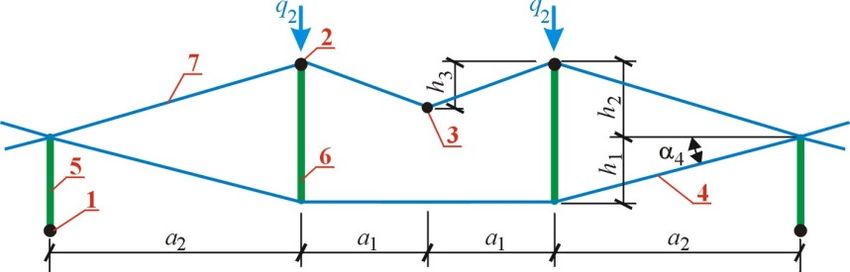
Proceedings of the TensiNet Symposium 2019
Softening the habitats. Sustainable Innovation in Minimal Mass Structures and Lightweight Architectures
______________________________________________________________________________________
Design & simulation of soft structures
Figure 2: View of the roof along the line a-a in figure 1 (Mikhaylov and Chesnokov, 2017).
Bearer cables are arranged in mutually perpendicular directions. Longitudinal bearer cables 1
are attached fixedly to columns. They are situated far from each other, allowing large free
areas to be ensured inside the building. Transverse bearer cables 4 are connected to struts 5,
which are, in turn, supported by the cables 1 and fixed by means of ties 8 in the longitudinal
direction. Backstay cables 2, supported by struts 6, are convex upwards. Together with ties 3
Soft Structures
and 7, they form the top chord of the roof.
The overall height of the roof is smaller in comparison to ordinary cable-membrane structures
of the same free span. Membrane curvature, however, is ensured to be in the appropriate
range. It allows the membrane to sustain external loads without wrinkles and slackened areas
(Forster, 2003).
2. Analysis of the structure
2.1. General considerations
The following parameters of the cable roof structure are taken into account:
− the modulus of elasticity and the strength of the cables and the struts Ecab , Rcab and Estr ,
Rstr respectively;
− cross section areas of the cables A j ( j = 1, 2, 3, 4 ), diameters of the struts D5 , D6
and their thickness-to-diameter ratios kt ,5 , kt ,6 ;
− cable tensioning L p ,1 , L p , 2 and L p ,3 ;
− the span of the primary bearer cables L, the distances between the cables a1 , a 2 and b,
initial sags of the cables f i ,0 and height dimensions hi ( i = 1, 2, 3 ).
73Proceedings of the TensiNet Symposium 2019
Softening the habitats. Sustainable Innovation in Minimal Mass Structures and Lightweight Architectures
______________________________________________________________________________________
Cable tensioning L p,i is implemented by means of an appropriate pre-stressing equipment
(Seidel, 2009). It is equal to the difference between, so called, geometrical length of the cable
Lсi , g and the length of the cable Lci , 0 in the unstressed state: L p,i = Lci, g − Lci,0 . The
geometrical length of the cable Lсi , g is determined by its shape in the initial state, excluding
any deflection of the structure: f = 0 .
Numbering of the structural elements is in the figures 1 and 2. Although the pre-stress may be
performed by means of the bottom cables 1 only (Mikhaylov and Chesnokov, 2017),
tensioning L p ,3 of the tie 3 results in more lightweight structure, due to the possibility of
force adjustment, which prevents the top chord from slackening. On the other hand,
embedding tensioning equipment into the cables 2 is not justified, so the value L p , 2 is
assumed equal to zero.
→
Cable cross section areas X = ( A1 , A2 , A3 , A4 )T and cable tensioning
→
L p = (L p,1 , L p,3 )T are taken as independent parameters, which are to be determined by
means of a structural optimization technique. Struts diameters D5 and D6 are also not
preliminary known, but they can be derived from the buckling prevention condition of
compressed structural members.
2.2. Flexible steel cable elements
Operability condition of the steel cables, constituting the roof structure, is taken into account
as follows:
lim,1 j lim, 2 (1)
where j is the ratio (2), while lim, 1 and lim, 2 are the limits of allowable range for the ratio:
Nj
j = (2)
A j Rcab
where N j is the force in the cable j.
The left-hand side of the condition (1) ensures, that the cable j is in tension and does not slack
under load, while the right-hand side prevents the cable from overstress.
74Proceedings of the TensiNet Symposium 2019
Softening the habitats. Sustainable Innovation in Minimal Mass Structures and Lightweight Architectures
______________________________________________________________________________________
Design & simulation of soft structures
The forces N j are calculated according to (Mikhaylov and Chesnokov, 2017), considering
A7 = A8 = A3 and q1 = q3 = 0 . They are obtained for the stage of pre-stress of the structure
N j , pr and for, so-called, operational stage N j , Ld , separately.
It is assumed, that the external load q 2 acts along the cable 2 from top to bottom, as shown in
the figures 1 and 2. For the operational stage the load is brought about by the structural own
weight, snow and suspended equipment: q2 = q . On the stage of the pre-stress the external
load is omitted due to its insignificance: q2 = 0 .
The force N 4 in the ordinary bearer cable 4 is obtained from the expression, given in
(Mikhaylov and Chesnokov, 2017), using uniformly distributed loads pi , acting on the cables
( i = 1, 2, 3 ). The forces in the primary bearer cable N1 , the backstay cable N 2 and the
longitudinal tie N 3 are obtained from the Hook’s law:
Soft Structures
N i = Ecab Ai i (3)
where i is the relative deformation of the cable, derived from (Chesnokov and Mikhaylov,
2017):
4 f i 4 + 2 f i 2 + L
i = i (fi , L p,i ) = −1 (4)
Lci ,0
where 2 and 4 are the coefficients, calculated for the middle of the span of the cable:
2 2.67 / L and 4 −6.4 / L3 ; fi = fi ,0 + fi is the cable sag; f i is the deflection of the
cable in the middle of the span, obtained from (Mikhaylov and Chesnokov, 2017); Lci , 0 is the
length of the cable in the unstressed state: Lci,0 = Lci, g − L p,i .
It is proposed to confine deformations of the roof under load by the following condition:
f 2, pr − f 2, Ld lim (5)
where lim is the limit value of the structural deflection; f 2, pr and f 2, Ld are the deflections
of the cable 2 brought about by pre-stressing of the roof and by the external load, respectively.
2.3. Compressed structural members
Diameters of the struts D5 and D6 are obtained from the conditions of compressive buckling
(6) and flexibility limitation (7):
75Proceedings of the TensiNet Symposium 2019
Softening the habitats. Sustainable Innovation in Minimal Mass Structures and Lightweight Architectures
______________________________________________________________________________________
N NE
(6)
lim (7)
where the index is either 5 or 6, depending on the strut considered, N E is the Euler load
(Galambos and Surovek, 2008), is the slenderness of the strut, lim = 120 is the limit
slenderness, N is the force in the corresponding strut:
N 5 = p1 b (8)
N 6 = N 4 sin( 4 ) (9)
Conditions (6) and (7) allow to derive the strut diameter:
8 N
(10)
D L 4
(
Estr kt , 1 − 3 kt , + 4 kt , 2 − 2 kt , 3
3
)
2 L
D (11)
lim kt , 2 − kt , + 0.5
where L is the length of the strut.
3. Structural optimization of the cable roof
Parameters of the cable roof form a multidimensional space, which consists of two sub-
spaces. The first one contains permissible parameter combinations p , while the second, or
invalid sub-space i describes the roof structure, which is either not operable or doesn’t
comply with the conditions imposed.
Permissible parameter groups p are not equivalent. Additional requirements, such as
material consumption, expenditures, labor input etc., distinguish them from each other,
resulting in the best combination, which should be determined. So, the problem of structural
optimization arises.
Complex behavior of the cable roof, reflected in slackening of compressed members and
instability of the structure in the whole, substantially complicates gradient optimization
techniques and diminishes their effectiveness. Among derivative-free, or zero-order,
approaches the coordinate descent method allows to gain reliable and numerically stable
76Proceedings of the TensiNet Symposium 2019
Softening the habitats. Sustainable Innovation in Minimal Mass Structures and Lightweight Architectures
______________________________________________________________________________________
Design & simulation of soft structures
results for the problem considered. It is accepted as a basis for the technique, elaborated in the
present work for estimation of cable roof structural parameters (figure 3).
Soft Structures
Figure 3: The technique for structural optimization of the cable roof
77Proceedings of the TensiNet Symposium 2019
Softening the habitats. Sustainable Innovation in Minimal Mass Structures and Lightweight Architectures
______________________________________________________________________________________
Parameters of the technique are the following: k is the number of current iteration and K lim is
→
the maximum number of iterations specified; X 0 is the vector of initially given values of
→
parameters to be optimized, while X k contains current parameter values; n = 4 is the number
→
of components of the vector X ; [ X lim ] is the matrix, which consists of n rows and 2 columns,
it contains allowable ranges for parameters to be optimized; [E ] is the identity matrix of n
→
rows and columns; s is a vector of n components, which contains possible variations of the
→ →
parameters; slim is a limiting value for a component of s ; is a reduction factor for s .
The criterion function is taken as follows:
→
Cr ( X ) = M cab + M str str (12)
where M cab and M str are total masses of the cables and the struts belonging to the structure
considered, str is the ratio of the average price of struts to the average price of cables.
→
According to the optimization technique only one component of the vector X is modified on
⎯→
⎯ ⎯⎯→
left right
each iteration step by means of decrementing X and incrementing X the current value.
→
Variations of the vector X are adjusted in order that the resultant vector components would
be in the appropriate range, specified by the matrix [ X lim ] .
→ →
Cable tensioning L p = (L p,1 , L p,3 )T , corresponding to the current vector X , is calculated
in the step-by-step way (figure 4).
→
Figure 4: Obtaining cable tensioning L p
→
The initial components of the vector L p are assumed equal to the increment
L p,1 = L p,3 = L p . If the condition (5) or the left-hand side of the condition (1) are not
78Proceedings of the TensiNet Symposium 2019
Softening the habitats. Sustainable Innovation in Minimal Mass Structures and Lightweight Architectures
______________________________________________________________________________________
Design & simulation of soft structures
satisfied, the increment L p is added to the corresponding component. However, if the right-
hand side of the condition (1) becomes not valid for any cable j, the step-by-step process is
→
terminated, and current X -vector is considered unacceptable.
The criterion function value (12) is saved into variable Y (figure 3). Negative Y-value means
either that current parameters are not permissible, or that the criterion function value is worse,
than the previously obtained result.
4. Case study
4.1. Initial data
The initial data taken into account are the following: the moduli of elasticity Ecab = 130 and
Soft Structures
E str = 206 GPa; the strength properties Rcab = 700 and Rstr = 240 MPa; dimensions of the roof
L = 12.0 m, a1 = 3.0 m, a2 = 3.0 m, b = 2 m, h1 = 1.0 m, h2 = 1.5 m, h3 = 0.8 m; initial sags of
the cables f1,0 = 1.0 m, f 2,0 = 1.0 m and f 3,0 = 0.7 m; thickness-to-diameter ratios of the struts
kt ,5 = kt ,6 = 1 / 20 ; the external load q = 10.8 kN/m; the limiting value for the structural
deflection lim = L / 150 = 0.08 m; the limiting values for the j -range (1): lim,1 = 0.1 and
lim, 2 = 1.0 .
The matrix of admissible ranges for parameters to be optimized is the following:
Alim, 1 Alim, 2
A Alim, 2
=
lim, 1
X lim (13)
Alim, 1 Alim, 2 / 5
Alim, 1 Alim, 2
where Alim, 1 = 22 mm2 and Alim, 2 = 1560 mm2 are the limiting cross section areas of the cables,
corresponding to the interval, which ranges from one cable with the diameter 6.1 mm and up
to two cables with the diameter 36.6 mm (PFEIFER, 2017).
→
Initial vector s of variations of parameters is obtained under the following expression:
→
su = ( X lim u,2 − X lim u,1) / 20 , where u = 1...n , n = 4 . The limiting value for s is adopted the
following: slim = 0.005 , while the maximum number of iterations is specified K lim = 500 . The
→
vector X 0 of initially given values for parameters is obtained under the following expression:
79Proceedings of the TensiNet Symposium 2019
Softening the habitats. Sustainable Innovation in Minimal Mass Structures and Lightweight Architectures
______________________________________________________________________________________
X 0u = ( X lim u ,1 + X lim u ,2 ) / 2 . The increment for the cable tensioning is adopted the following:
L p = 0.01 . The price ratio is taken the following: str = 1 / 3 .
4.2. Comparison with results, obtained by the licensed software for non-linear structural
analysis
→
The following X -vector (1) is obtained by means of the iteration technique (figure 3):
→
X = (4.42 2.14 0.22 1.54 )T cm2 (14)
→
The corresponding L p -vector is the following:
→
L p = (0.1248 0.0347 )T m (15)
Diameters of the struts, obtained from (10) and (11), are the following: D5 = 31 mm and
D6 = 62 mm.
The criterion function value (12) is 254.7. The masses of cables and struts, belonging to the
structure considered, are the following: M cab = 213 .6 and M str = 123 .3 kg.
In order to verify the proposed technique, structural analysis of the cable roof was performed
by means of the specialized software package EASY. The comparison of results is
accomplished by the following expression:
e − p
= 100 (16)
0.5 e + p
where is the relative discrepancy, %; is the structural parameter to be compared; indexes
“e” and “p” refer to the results, obtained by the EASY software and by the proposed
formulations, respectively.
Comparison of forces in the cables j = 1, 2, 3, 4 and in the struts 5 and 6 are in the tables
1 and 2. The forces are given in kilonewtons. The deflections of the primary bearer cable 1
and the backstay cables 2, obtained in two ways, are very close to each other:
p p p p
f 1, pr = −0.2024 m, f 1, Ld = −0.1493 m, f 2, pr = 0.1436 m, f 2, Ld = 0.0636 m, and
e e e e
f 1, pr = 0.2050 m, f 1, Ld = 0.1518 m, f 2, pr = 0.1495 m, f 2, Ld = 0.0690 m. Corresponding
discrepancies (16) are the following: 1, pr = 1.3 %, 1, Ld = 1.7 %, 2, pr = 4.0 % and 2, Ld = 8.1 %.
80Proceedings of the TensiNet Symposium 2019
Softening the habitats. Sustainable Innovation in Minimal Mass Structures and Lightweight Architectures
______________________________________________________________________________________
Design & simulation of soft structures
p p
Remark: the deflections f 1, pr and f 1, Ld are multiplied by -1.0 before substitution into
(16), because positive displacements of the cable 1, assumed in the present paper and in the
EASY software are opposite to each other.
Table 1: Comparison of forces in the cables
Load-
N p1 N e1 p1 N p2 N e2 p2 N p3 N e3 p3 N p4 N e4 p4
case
Pre-stress 218.8 212.7 149.6 143.9 9.65 9.80 63.5 60.0
0.70 1.00 0.62 0.60
only 1, pr = 2.8 % 2, pr = 3.9 % 3, pr = 1.6 % 4, pr = 5.7 %
Pre-stress 309.1 301.8 64.1 59.5 1.54 1.68 92.6 86.0
and
1.00 0.43 0.10 0.86
vertical 1, Ld = 2.4 % 2, Ld = 7.4 % 3, Ld = 8.7 % 4, Ld = 7.4 %
load q
Soft Structures
Table 2: Comparison of forces in the struts
Load- N E ,5 5 N E ,6 6
N p5 N e5 N p6 N e6
case
Pre-stress 19.37 19.26 20.1 19.9
only 5, pr = 0.6 % 6, pr = 1.0 %
Pre-stress 29.2 28.8 31.7 95.9 29.3 29.2 81.1 120.0
and
vertical 5, Ld = 1.4 % 6, Ld = 0.3 %
load q
Remark: NE and are designated in the expressions (6) and (7).
5. Conclusion
Cable roof structure intended for large-span buildings is considered. In spite of comparatively
reduced overall height, the roof ensures the membrane covering to be of a required curvature
in order to avoid wrinkles and slackened areas.
Numerical technique, based on the coordinate descent method, is used to perform structural
optimization. The technique is numerically stable and allows to gain reliable solutions for the
problem, multidimensional parameter space of which includes, so-called, invalid sub-spaces
i . It allows to determine pre-stress values and stiffness properties of structural members,
needed for automated computer simulation of the construction. In comparison to graphical
approach, used in the previous work, the technique proposed in the present paper is much
more effective, providing reliable results in a short period of time.
81Proceedings of the TensiNet Symposium 2019
Softening the habitats. Sustainable Innovation in Minimal Mass Structures and Lightweight Architectures
______________________________________________________________________________________
The future improvement of the optimization technique should be in the field of cost estimation
refinement, including expenditures for manufacturing and installation of the cable roof in the
whole and also particular joints and details.
References
Chesnokov A.V. and Mikhaylov V.V. (2016), Cable roof structure. Utility Model Patent
RU169612, (in Russian). Retrieved January 8, 2019, from http://new.fips.ru/en/.
Chesnokov A.V. and Mikhaylov V.V. (2017), Analysis of cable structures by means of
trigonometric series. In: Proceedings of the VIII international conference on textile
composites and inflatable structures. Munich, 9-11 October 2017, (pp. 455 – 466).
Forster B. (2003), Engineered fabric architecture – characteristics and behaviour. In:
Proceedings of the TensiNet symposium. Brussel, 19-20 September, 2003, (pp. 28 – 43).
Galambos T.V. and Surovek A.E. (2008), Structural stability of steel: concepts and
applications for structural engineers. New Jersey: John Wiley and Sons.
Goppert K. (2013). High tension tensile architecture. New stadium projects. In: Proceedings
of the VI International conference on textile composites and inflatable structures. Munich, 9-
11 October 2013, (pp. 21-26).
Grunwald G. and Seethaler M. (2011). Reconstruction. Olympic stadium. Kiev, Ukraine. In:
Tensinews N21, (pp. 9 – 10).
Houtman R. (2003), There is no material like membrane material. In: Proceedings of TensiNet
symposium. Brussel, 19-20 September, 2003, (pp. 178 – 194).
Mikhaylov V.V. and Chesnokov A.V. (2017), Cable roof structure with flexible fabric
covering. In: Proceedings of the VIII international conference on textile composites and
inflatable structures. Munich, 9-11 October 2017, (pp. 436 – 447).
PFEIFER Tension Members (2017): PFEIFER seil- und hebetechnik GMBH. Retrieved
January 8, 2019, from https://www.pfeifer.info/en/pfeifer-group/business-units/cable-
structures/.
Seidel M. (2009). Tensile Surface Structures: A Practical Guide to Cable and Membrane
Construction: Ernst and Sohn.
82You can also read