On Wind Speed Sensor Configurations and Altitude Control in Airborne Wind Energy Systems
←
→
Page content transcription
If your browser does not render page correctly, please read the page content below
On Wind Speed Sensor Configurations and Altitude Control
                                                                 in Airborne Wind Energy Systems
                                                            Laurel N. Dunn1,3 , Christopher Vermillion2 , Fotini K. Chow1 , and Scott J. Moura1

                                              Abstract— Real-time altitude control of airborne wind energy              known wind resources (exploitation) and collecting obser-
                                           (AWE) systems can improve performance by allowing turbines                   vations at altitudes where wind speed estimates are uncer-
                                           to track favorable wind speeds across a range of operating                   tain (exploration), given that wind speed profiles are only
                                           altitudes. The current work explores the performance implica-
                                           tions of deploying an AWE system with sensor configurations                  partially observable and that altitude adjustments are costly
arXiv:2001.07591v1 [eess.SY] 21 Jan 2020

                                           that provide different amounts of data to characterize wind                  to make. Over time, control decisions favoring exploration
                                           speed profiles. We examine various control objectives that                   can reduce uncertainty in wind speed models, though doing
                                           balance trade-offs between exploration and exploitation, and                 so may come at a cost to near-term performance. We refer
                                           use a persistence model to generate a probabilistic wind                     readers to [12] for information on Bayesian optimization
                                           speed forecast to inform control decisions. We assess system
                                           performance by comparing power production against baselines                  and a more detailed discussion of the trade-off between
                                           such as omniscient control and stationary flight. We show that               exploration and exploitation.
                                           with few sensors, control strategies that reward exploration                    In the context of AWE system altitude control, this trade
                                           are favored. We also show that with comprehensive sensing,                   off is directly related to uncertainty in wind speed estimates
                                           the implications of choosing a sub-optimal control strategy                  that inform control decisions. A survey of state-of-the-art
                                           decrease. This work informs and motivates the need for future
                                           research exploring online learning algorithms to characterize                algorithms for forecasting wind power production is given in
                                           vertical wind speed profiles.                                                [13]. Many of the algorithms cited require large training data
                                                                                                                        sets. Training such algorithms may not be possible for AWE
                                                        I. I NTRODUCTION AND M OTIVATION                                systems which typically rely on sparse data streams collected
                                              Airborne wind energy (AWE) turbines are an emerging                       online. Observations are sparse because wind speeds are
                                           wind generation technology. AWE systems differ from con-                     recorded by a single sensor that tracks (vertically) with the
                                           ventional turbines in that they are attached to the ground                   operating altitude of the turbine. A simpler persistence model
                                           by an adjustable tether, rather than by a fixed tower. This                  is also shown to perform quite well, and is recommended as a
                                           tethered design reduces capital costs and makes it possible                  benchmark for evaluating the performance of more complex
                                           to achieve a higher capacity factor. We refer readers to [1] for             wind forecasting algorithms.
                                           an in-depth description of airborne wind energy. Information                    Aside from using complex forecasting algorithms, un-
                                           about modern AWE systems can be found at [2], [3], [4].                      certainty in wind speed can be reduced by increasing the
                                              Three characteristics of AWE systems contribute to a high                 spatial coverage of wind speed sensors. For example, if
                                           capacity factor compared with conventional turbines. First,                  wind speeds were recorded continuously at all altitudes, a
                                           AWE systems can reach higher altitude winds, which tend to                   simple forecasting model (e.g. the persistence model) may
                                           be stronger and more consistent than surface-level winds [5].                be able to outperform a system that uses a more sophisticated
                                           Second, AWE systems can use crosswind flight patterns to                     forecasting model trained on single sensor data. This possi-
                                           increase the apparent wind speed [6], leading to more power                  bility motivates a comparative analysis of different sensor
                                           output than would be achieved with stationary flight [7],                    configurations and forecasting methods for AWE altitude
                                           [8]. Finally, by adjusting the operating altitude in real-time,              control, an issue currently unexplored in the literature.
                                           AWE systems can vertically track favorable wind speeds                          The main contribution of the current work is to develop a
                                           in a spatially and temporally varying wind field [9]. The                    framework for evaluating performance gains achievable using
                                           current work focuses on understanding how sensor placement                   different wind speed sensor configurations. We demonstrate
                                           impacts the performance of an AWE system with various                        this framework with a case study of a particular wind
                                           altitude control schemes.                                                    field. We use the control objectives proposed in [11] to
                                              Currently, research on AWE altitude control systems focus                 determine the optimal altitude trajectory. Questions related
                                           on control schemes that find the optimal operating altitude                  to the performance gains from coupling sensor data with
                                           [10] and are robust to uncertainty [11]. For example, [11]                   different statistical forecasts are reserved for future research.
                                           borrow control objectives from Bayesian optimization to                         This paper is organized as follows. Section II provides
                                           balance exploration and exploitation. More specifically, these               methodological details. Section III outlines the sensor config-
                                           objectives balance the trade off between capitalizing on                     urations. Section IV details the forecasting methods. Section
                                                                                                                        V formulates the altitude control objectives. Section VI
                                              1 Department of Civil & Environmental Engineering, University of Cali-
                                                                                                                        describes the comparative analysis benchmarks and metrics.
                                           fornia Berkeley
                                              2 Department of Mechanical Engineering, North Carolina State University   Section VII provides the results and discussion. Finally,
                                              3 Corresponding author: lndunn@berkeley.edu                               Section VIII summarizes the paper’s main conclusions.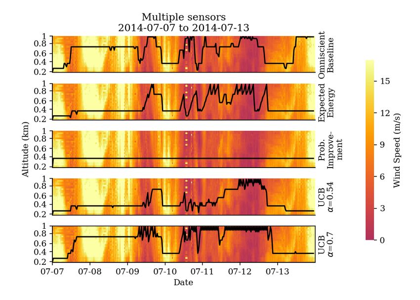
still considered partially observable as wind speeds are not
measured above the hub height. However, flying the turbine
at the highest altitude within operating bounds would provide
a complete wind speed profile.
The focus of the current work is to assess the performance
implications rather than to explore sensor technologies them-
selves. However, we have identified several technologies that
could collect these measurements. One option is to affix
anemometers in regular intervals along the tether, which
provides reliable wind speed measurements at altitudes below
the AWE system but requires a winch system to house the
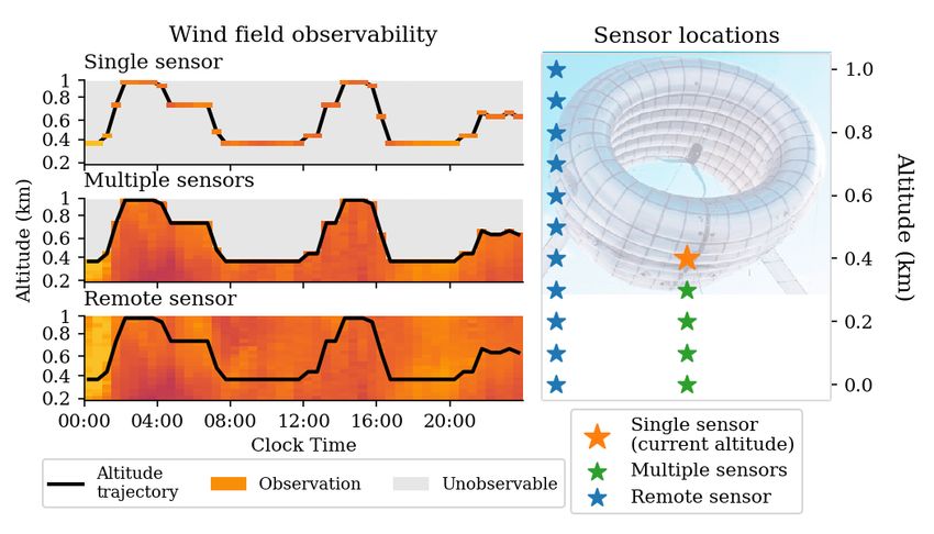
Fig. 1. Schematic diagram showing wind field measurements recorded anemometers upon spool-in. Another alternative is to attach
by each of three sensor configurations. Right panel shows measurement telltales to the tether and use image processing to estimate
locations for single, multiple, and remote sensor configurations. Left panel wind speeds from the angle of the telltale relative to the
shows the altitude (y-axis) and magnitude (color scale) of the measurements
that would be recorded by each sensor configuration given some trajectory tether. Finally, one could potentially compute local wind
(black line) of altitudes with respect to time (x-axis). velocities based on the catenary geometry of the tether,
though to do so would require a detailed characterization
of the tether’s structural and aerodynamic properties. Further
II. M ETHODS research is needed to assess the technical and economic feasi-
In this work we simulate the altitude trajectory of a bility of specific solutions for collecting these measurements.
buoyant airborne turbine (pictured in Fig. 1) in a spatially and
C. Remote sensor configuration
temporally varying wind field. The simulation relies on wind
speed data recorded by a 915-MHz wind profiler between The third configuration relies on a remote sensor to record
July 1, 2014 and August 31, 2014 at Cape Henlopen State wind speed measurements in discrete intervals across a
Park in Lewes, DE [5]. Wind speed data are measured every wide range of altitudes simultaneously. For example, the
50 meters in 30 minute intervals. We use the same spatial wind data we use to inform our simulation was collected
and temporal discretization in simulation. using a vertical profiler that measures wind speeds in 50
We examine single-sensor, multiple-sensor and remote meter increments. With remote sensing wind speed profiles
sensor configurations. We track the wind speed measure- are fully observable at each time step. Because the same
ments that would be recorded online given a particular measurements are recorded regardless of the current position
sensor configuration and the altitude trajectory followed of the turbine, this configuration decouples data acquisition
up to a particular point in time. Observations are used to from altitude control. The implication is that exploring the
train a persistence model that generates a probabilistic wind wind field for data acquisition is not necessary, and that
speed forecast. We use three different control objectives to control decisions can focus instead on exploitation of known
determine the optimal altitude trajectory given the current wind resources.
wind speed forecast. IV. P ERSISTENCE F ORECAST
Altitude trajectories are generated for a range of scenarios,
We use a persistence model adapted from [13] to generate
each of which uses:
a probabilistic wind speed forecast. We extend the model
1) One of three control objectives to extrapolate wind speeds into the spatial domain, and to
2) One of three sensor configurations characterize uncertainty. The persistence model is based on
3) A persistence forecast the premise that wind speeds change very little (or not at all)
The current work examines differences in power production from one time step to the next. The spatial extension of this
with each sensor configuration. We build on the control model presumes that there is little (or no) change vertically
objectives presented in [11] to do so, and leave it to future either. Based on this premise, the forecast mean µ at altitude
work to explore the performance implications of using more h and s time steps into the future is given by:
sophisticated wind forecasting methods.
III. S ENSOR CONFIGURATIONS µh,t+s = Xt (h0 ) (1)
A. Single-sensor configuration where Xt (h) describes the wind speed observation recorded
AWE systems are typically designed with a single at time t and altitude h. We define h0 to be the measurement
anemometer to measure the wind speed at the current op- altitude in Xt that is either equal to the forecast altitude
erating altitude. The vertical position of these measurements h, or is nearest to it. For example, with multiple sensors, h0
changes when altitude adjustments are made. would be equal to h for altitudes below the current operating
altitude, and would equal the current altitude (i.e., the highest
B. Multiple sensor configuration observable altitude) otherwise. The fundamental assumption
A novel sensor design would be to record wind speed is that the measurement Xt (h0 ) recorded at (h0 , t) persists
measurements along the length of the tether. The system is across all unobserved times and altitudes.TABLE I
We characterize uncertainty by estimating how erroneous
L IST OF MODEL PARAMETERS AND VALUES .
the assumption of persistence could be based on past obser-
Variable Value
vations. We define ∆ to be a matrix composed of column
hmin 0.15 km
vectors ∆X/∆h and ∆X/∆t describing the finite differ- hmax 1.0 km
ences between measurements in X in space and time. Based rmax 0.01 km/min
on an exploratory analysis of the data, we characterize ∆ as vr 12 m/s
∆t 30 min
a joint Gaussian distribution with zero mean. T 90 min
Next, we define the vector d describing the distance in k1 0.0579 kW s3 /m3
space (h−h0 ) and in time (s) between the current observation k2 0.09 kW s2 /m2
k3 1.08 kW s2 /m2 · km
(Xt (h0 )) and the forecast. We can then characterize forecast
uncertainty (σ 2 ) as:
2
= Σ d∆T = dΣ(∆)dT
σh,t+s (2) planning horizon is sufficient for the turbine to travel between
any two operating altitudes. We use dynamic programming
Here Σ(∆), for example, is the covariance of ∆.
to solve for the optimal trajectory at each time step.
Where forecast uncertainty is high, we truncate the distri-
We examine three formulations of g(h, u, V ) that aim to
bution between 0 and 17 m/s to ensure that high uncertainty
maximize power production. These formulations differ in
does not lead to unrealistic predictions. We find that 98%
how they account for uncertainty in power production (which
of all observations in the data are within these bounds. We
stems from uncertainty in wind speed forecasts). Although
assume that the underlying distribution of ∆ is stationary,
the objective function differs for each formulation, the long-
though characterizing non-stationarity in wind speed dynam-
term goal is always to maximize power production.
ics presents an interesting opportunity for future work.
Equation (6) lists the system of equations used to calculate
V. C ONTROL M ETHODS power production, as described in [10]. Here power produc-
We describe altitude control using the following simple tion p(u(t), v) is a function of the altitude adjustment during
integrator dynamics: some time interval u(t) and the true wind speed v.
h(t + 1) = h(t) + u(t) (3)
p(u, v) = p1 − p2 − p3
where h(t) is the altitude at discrete time index t, and u(t) p1 = k1 · min{vr , v}3
is the controlled altitude adjustment. (6)
p2 = k2 v 2
The control objective at a given time t is to select the
trajectory of optimal future operating altitudes {h∗ (t + p3 = k3 v 2 · |u|
1), h∗ (t + 2), · · · } and controlled altitude adjustments in
In words, the total power production p(u, v) is the differ-
{u∗ (t), u∗ (t + 1), · · · } that maximize some objective func-
ence between the amount of energy the turbine generates
tion, given the wind speed forecast V . We express this
(p1 ) and the amount of energy required to maintain (p2 )
objective J mathematically as:
and to adjust (p3 ) the operating altitude. The rated wind
t+T
X speed of the turbine is given by vr , and k1 , k2 and k3
max J = g(h(s), u(s), V∀h,s ) (4) describe lumped parameters representing the mechanical and
h(t),u(t)
s=t aerodynamic properties of the system. Numeric values for
Here V∀h,s to refers collectively to the random wind speed these constants are provided in Table I.
forecasts for all candidate altitudes h at time s, and T is the We highlight that p1 is maximized when v is equal to
planning horizon. vr . However, p2 and p3 continue to increase at wind speeds
The problem is constrained such that operating altitudes greater than vr . The implication is that p(u, v) increases as
are bounded to within hmin and hmax , and the rate of change v approaches vr , but decreases if v increases beyond vr .
in altitude is below rmax . The wind speed v can represent either a measurement
hmin ≤ h(t) ≤ hmax reported in the data, or some realization of the wind speed
(5) forecast. In order words, if Vh,t is a random variable describ-
|u(t)| ≤ rmax ing the wind forecast at altitude h and time t, then we can use
Table I provides numerical values for operating constraints. the function p(·) to derive a probabilistic forecast of power
This formulation uses model predictive control to optimize production, denoted by Ph,t . Though Ph,t is not explicitly
the control and state trajectories over the upcoming T time- related to h or t, it is implicitly related by the fact that the
steps given the current state h(t), dynamical model (3) and wind forecast changes with respect to both quantities.
wind speed forecasts for all altitudes. Only the first control In the following sections we describe three candidate
action u∗ (t) is physically implemented, and the process is formulations of g(h, u, V ). Though the specific objective
repeated using the measured state in the next time step. functions are different, the aim of all three formulations
We use a planning horizon of 90 minutes (or three 30- is to maximize overall power production. The objective
minute time steps). Given the values listed in Table I, the functions are borrowed from Bayesian optimization, and theirapplication to real-time control of AWE systems is motivated power production. Tuning the upper confidence bound α
in [11]. adjusts the degree to which exploration is rewarded. The
Though the formulations we use are conceptually the drawback is that when an overly optimistic control objective
same as the control objectives presented in [11], we have is used (i.e., if α is close to 1), there is a high risk that
adapted them in two important ways. First, we optimize over the observed power production will be much lower than the
a finite planning horizon extending T time steps into the value used to inform a control decision.
future. Second, we use a probabilistic wind speed forecast Algorithms favoring exploration may under-perform rel-
to compute a probability distribution of power production. ative to purely exploitative methods, except insofar as they
Since power production is a nonlinear function of wind reward acquisition of new data that reduces long-run uncer-
speed, the power production is not Gaussian, and generally tainty in the wind speed forecasts. As uncertainty bounds
does not follow a parametric distribution. As shown below, become narrow, the difference in power production between
our approach handles non-parametric distributions directly, control objectives favoring exploration and exploitation also
and does not require parametric approximations. decreases.
A. Maximize Expected Energy C. Maximize Probability of Improvement
The first control strategy chooses the altitude trajectory The last control strategy selects the altitude trajectory with
that maximizes expected power production across time steps the highest probability of improving performance relative to
within the planning horizon. This can be viewed as an maintaining the current altitude. We calculate the probability
exploitative control approach, in the sense that no reward of improvement by taking the log probability that power
is explicitly provided to explore portions of the state-space production for a particular trajectory will exceed power
where uncertainty is high. Instead, the goal is to directly production if the altitude were to remain fixed at current
maximize expected power production. altitude h. Mathematically, this is expressed in (10).
In continuous form, the expected power at time t is given
g(h, u, V ) = log Pr (Ph+u,t > p(0, v)) (10)
by (7), where fVh,t (v) is the probability density function
(PDF) of wind speed forecast random variable Vh,t . where Ph+u,t = p(u, Vh,t ) is a random variable describing
Z ∞ power generation at altitude h + u, and p(0, v) is the current
E[Ph,t |u, Vh,t ] = fVh,t (v)p(u, v)dv (7) power output (i.e. no altitude adjustment u = 0 and assuming
0 wind speed v stays constant).
To accommodate non-parametric wind speed forecasts
VI. P ERFORMANCE M ETRICS AND BASELINE
with no closed form solution to (7), we use the discrete
S CENARIOS
approximation given by
n In the current section we define metrics and benchmarks
1X to evaluate the performance of each sensor configuration and
E[Ph,t |u, Vh,t ] ≈ p(u, vq/n )
n q=1 control strategy. We calculate these metrics and benchmarks
(8) by simulating the altitude trajectory over the course of three
vq/n = QVh,t (q/n)
months.
QVh,t (q/n) := Pr(Vh,t ≤ v) = q/n
A. Performance metrics
Here QY (q/n) is the inverse cumulative density function
(CDF) of some random variable Y evaluated at quantile q for The most fundamental metric we use to evaluate perfor-
a specified number of quantile bins n. For example, QY (q/n) mance is average power production (in kW). Though power
evaluates to the q th quartile of Y when n is 4, or to the q th production could be compared against the nameplate capacity
percentile when n is 100. We set n equal to 100. (in this case 100 kW), this is not a practical target as it is not
physically possible to achieve that level of performance. A
B. Maximize Upper Confidence Bound (UCB) more practical target would need to account for the physics
The second control strategy chooses the altitude trajectory of the simulation environment, including variations in wind
that maximizes performance under an optimistic realization speed and the energy required to adjust and maintain altitude.
of the forecast. This is also known as quantile optimization. The omniscient baseline (described below) provides just
For example, one might maximize the 90th percentile of Ph,t . such a target. In addition to reporting power production,
Equation (9) expresses this mathematically for an arbitrary we express performance as a ratio (between 0 and 1) of
probability threshold α > 0.5 and usually near 1. the energy harvested in a particular scenario and the energy
harvested in the omniscient baseline. We refer to this quantity
g(h, u, V ) = QPh,t |u,Vh,t (α|u, v) (9) as the “actualized power ratio” (as in Figs. 3 and 4).
where QPh,t |u,Vh,t describes the inverse conditional CDF of B. Performance baselines
the random variable Ph,t conditioned on u = u and Vh,t = v. 1) Omniscient baseline: The omniscient baseline is ob-
This approach rewards trajectories that explore altitudes tained by simulating the altitude trajectory the AWE would
where uncertainty may be large yet potentially yields high follow if perfect information were available to inform controldecisions. The result provides an upper limit on power
production, given the characteristics of the wind field and
the specified operating constraints.
2) Fixed altitude baseline: We also compare our results
against baselines where the altitude is fixed for the entire
of the simulation at the altitudes that would achieve the
highest (hbest ) and lowest power production (hworst ). Though
these provide a useful basis for comparison, we note that
it is not possible to know hbest or hworst without omniscient
information about the wind speeds at each altitude.
Unlike the omniscient baseline, fixed altitude trajectories
do not bound system performance. Instead, they provide a
benchmark against a naı̈ve, but possibly effective, control
strategy. A real-time control scheme can under-perform rela-
tive to a fixed altitude trajectory if control decisions are made
based on sufficiently erroneous wind speed forecasts, or if Fig. 2. Altitude trajectory of AWE turbine (black line) over one week (July
the power production observed at the new operating altitude 7-13, 2014) for control scenarios indicated on the right. We include UCB
control scenarios where α = 0.54 (the optimal), and α = 0.7 (included
does not compensate for the energy expended in making the for illustrative purposes). The color scale indicates the wind speed at each
altitude adjustment. altitude (y-axis) with respect to time (x-axis).
VII. R ESULTS AND D ISCUSSION
as to improve performance. Thus the probability of improve-
Here we summarize the performance of an AWE system ment is only 50%, and control decisions favor maintaining
evaluated in simulation for nine scenarios. What differen- a constant altitude to avoid power loss from making altitude
tiates each scenario is the specific combination of sensor adjustments.
configuration and control scheme used to inform altitude ad- Though the objective to maximize expected energy is also
justments. A persistence forecast is trained on observational centered about the current observation, control decisions in
data collected in simulation, given the sensor configuration that case are informed not only by the probability but also the
and altitude trajectory up to that point. We examine a range magnitude of improvement potential. Since the magnitude of
of values for α in the upper confidence bound (UCB) control improvement scales with v 3 , the distribution of p is skewed
and report results for the value that achieves the highest to the right and there is some incentive to explore.
performance in each sensor configuration. We compare the Observation 3: In the multi-sensor case, when the ob-
performance in each scenario against the omniscient and jective is to maximize the upper confidence bound (UCB),
fixed altitude baselines. trajectories tend towards higher altitudes rather than lower
Fig. 2 shows the altitude trajectory over one week in altitudes. This happens because the uncertainty is greater
August for the omniscient baseline and four control schemes at unobserved altitudes above the current hub height than
in the multiple-sensor scenarios. Commenting on the simi- at altitudes where current measurements are available. This
larities and differences between trajectories highlights the high uncertainty creates a strong incentive to explore higher
merits (and pitfalls) of using a particular control scheme with altitudes. However, once the highest altitude is reached, the
each sensor configuration. system becomes completely observable and uncertainty is
Observation 1: Though altitude trajectories follow very equal at all altitudes, so exploitation is favored.
different patterns at times when the wind speed is low (e.g., At this point the trajectory will tend downwards if the best
July 11-13), they all follow a relatively fixed course when wind resource is below the uppermost altitude. Decreasing
wind speeds are high (e.g., July 8-9). The reason for this is the hub height also makes the system only partially ob-
that p1 is constant for wind speeds in excess of vr , while servable, reinstating the reward to explore higher altitudes.
p2 and p3 continue to increase. The incentive to explore is This process repeats, causing the oscillations observed in the
only in place if the potential increase in power production lowermost panel in Fig. 2. These oscillations come at a high
exceeds the cost of making altitude adjustments. When the energy cost and do not necessarily lead to gains in overall
wind speeds are near or in excess of vr , a fixed altitude is performance. We examine how energy is allocated when α is
favored because exploration comes at a relatively high cost set to 0.7, and compare it against energy allocation when the
without the possibility of increasing power production. optimal value (0.54) is used. Although the higher incentive
Observation 2: Maximizing the probability of improve- to explore leads to a 4% increase in power production
ment leads to a fixed altitude trajectory in both the single- (p1 ), the system expends twice as much energy on altitude
and multiple-sensor cases. The reason for this is that wind adjustments (p3 ). The additional energy cost leads to a
speed forecasts are centered around the current observation. 3% reduction in overall performance. Fig. 3 shows that
In other words, the forecast estimates that exploring some performance tends to decrease as α increases.
unobserved altitude is equally likely to reduce performance Fig. 4 summarizes overall power production across theuncertainty in the forecast is incorporated into the control
objective.
We demonstrate that an AWE system with remote sensing
equipment can achieve a high level of performance using
the most recent measurement to inform control decisions.
As the amount of information available to characterize wind
speed profiles decreases, forecast uncertainty increases and
performance declines.
Fig. 3. Average power production (y-axis) for upper confidence bound Both results are related to the quality of the wind speed
control scenarios, as a function of confidence level α (x-axis).
forecast, raising the question: Can a high-fidelity statistical
model improve performance and/or close the gap in perfor-
mance between different sensor configurations? Our work
underscores the need for further research exploring statistical
methods for characterizing vertical wind speed profiles.
ACKNOWLEDGEMENTS
This work was supported by the National Science Founda-
tion under Award 1437296. The authors would like to thank
Cristina Archer at the University of Delaware for providing
the wind speed data used in this study.
Fig. 4. Average power production for each control scheme & sensor
configuration. Horizontal lines denote omniscient baseline (solid line), and
the best (dashed line) and worst (dotted line) fixed altitude trajectories.
R EFERENCES
Performance is measured in terms of average power production (left y-axis) [1] M. Diehl, Airborne Wind Energy: Basic Concepts and Physical
and in terms of the “actualized power ratio” between power production and Foundations. Berlin, Heidelberg: Springer Berlin Heidelberg,
the omniscient baseline (right y-axis). 2013, pp. 3–22. [Online]. Available: https://doi.org/10.1007/
978-3-642-39965-7 1
[2] Website, accessed: Sept 24, 2018. [Online]. Available: http:
//www.altaeros.com/
three-month simulation in all nine scenarios, and compares [3] Website, accessed: Sept 24, 2018. [Online]. Available: https:
them against baselines presented in Section VI. //www.skysails.info/
[4] Website, accessed: Sept 24, 2018. [Online]. Available: http:
Our results show that the remote sensor improves perfor- //www.ampyxpower.com/
mance by 11% compared with deploying the system with [5] C. L. Archer, “Wind profiler at cape henlopen,” Website, accessed:
multiple sensors, and by 15% compared with deploying a Sept 23, 2018. [Online]. Available: https://www.ceoe.udel.edu/
our-people/profiles/carcher/fsmw
system with only a single sensor. Fig. 3 shows that although [6] M. L. Loyd, “Crosswind kite power,” J. Energy, vol. 2, no. 80-4075,
performance declines as α increases, the remote sensor 1980.
consistently outperforms the other two sensor configurations. [7] L. Fagiano, A. U. Zgraggen, M. Morari, and M. Khammash, “Auto-
matic crosswind flight of tethered wings for airborne wind energy:
In all scenarios the multiple and single-sensor cases perform Modeling, control design, and experimental results,” IEEE Transac-
about on par with the optimal altitude (hbest ) for stationary tions on Control Systems Technology, vol. 22, no. 4, pp. 1433–1447,
control. In practice, however, it is not possible to know hbest July 2014.
[8] P. Nikpoorparizi, N. Deodhar, and C. Vermillion, “Modeling, control
in advance. design, and combined plant/controller optimization for an energy-
These results are based on the highest performing control harvesting tethered wing,” IEEE Transactions on Control Systems
strategy for each sensor configuration. However, the optimal Technology, vol. 26, no. 4, pp. 1157–1169, July 2018.
[9] C. L. Archer, L. D. Monache, and D. L. Rife, “Airborne wind energy:
value for α is not known a priori, and likely depends Optimal locations and variability,” Renewable Energy, vol. 64, pp.
on many factors such as the spacing of sensors and the 180 – 186, 2014. [Online]. Available: http://www.sciencedirect.com/
characteristics of the wind field. Fig. 3 shows that the science/article/pii/S0960148113005752
[10] A. Bafandeh and C. Vermillion, “Real-time altitude optimization of air-
consequences of choosing a sub-optimal control strategy are borne wind energy systems using lyapunov-based switched extremum
particularly severe in the multiple sensor configuration. seeking control,” in 2016 American Control Conference (ACC), July
2016.
Finally, Fig. 3 shows that heavily rewarding exploration [11] A. Baheri, S. Bin-Karim, A. Bafandeh, and C. Vermillion, “Real-time
may slightly improve performance in the single-sensor con- control using bayesian optimization: A case study in airborne wind
figuration, but actually decreases performance in the multi- energy systems,” Control Engineering Practice, vol. 69, pp. 131 –
140, 2017. [Online]. Available: http://www.sciencedirect.com/science/
sensor configuration. This decline in performance is due to article/pii/S0967066117302101
the altitude oscillations discussed in Observation 3. [12] E. Brochu, V. M. Cora, and N. de Freitas, “A tutorial on bayesian
optimization of expensive cost functions, with application to active
user modeling and hierarchical reinforcement learning,” CoRR, vol.
VIII. C ONCLUSIONS AND F UTURE W ORK abs/1012.2599, 2010. [Online]. Available: http://arxiv.org/abs/1012.
2599
In this work we report on differences in AWE perfor- [13] S. S. Soman, H. Zareipour, O. Malik, and P. Mandal, “A review of
mance achieved in simulation using various different control wind power and wind speed forecasting methods with different time
horizons,” in North American Power Symposium 2010, Sept 2010, pp.
strategies and wind speed sensor configurations. The key 1–8.
difference between the control strategies is how (or if)You can also read