One Pose Fits All A Novel Kinematic Approach to 3D Human Pose Estimation Yen-Lin Wu - TU Delft Repositories
←
→
Page content transcription
If your browser does not render page correctly, please read the page content below

One Pose Fits All A Novel Kinematic Approach to 3D Human Pose Estimation Yen-Lin Wu


One Pose Fits All
       A Novel Kinematic Approach to
        3D Human Pose Estimation
                                        by

                            Yen-Lin Wu
                     to obtain the degree of Master of Science
                         at Delft University of Technology,
         to be defended publicly on Monday August 23rd, 2021 at 2:00 PM.

      Student number:      4848489
      Project duration:    November 1, 2020 – August 23, 2021
      Thesis committee:    Dr. Jens Kober,     TU Delft, Chair & Supervisor
                           Dr. Osama Mazhar, TU Delft, Daily supervisor
                           Dr. Julian Kooij,   TU Delft, External Member

An electronic version of this thesis is available at http://repository.tudelft.nl/.

Abstract

3D human pose estimation is a widely researched computer vision task that could be ap-
plied in scenarios such as virtual reality and human-robot interaction. With the lack of
depth information, 3D estimation from monocular images is an inherently ambiguous prob-
lem. On top of that, unrealistic human poses have been overlooked in the majority of pa-
pers since joint detection is the only focus.

   Our work consists of two parts, an end-to-end 2D-3D lifting pipeline and a novel kine-
matic human model integrated approach. We start with Pose Estimation using TRans-
former (PETR), an approach that does not require temporal information and has the at-
tention mechanism to model the inter-joint relationship from RGB images.

    In the approach with human model, we emphasize pose similarity rather than focusing
on joint detection. We propose a new metric, called Mean Per Bone Vector Error (MPBVE),
that evaluates poses regardless of a human body’s gender, weight, or age. We introduce
Pose Estimation on Bone Rotation using Transformer (PEBRT), a novel approach that re-
gresses rotation matrices for 16 human bones, assuming labeled 2D poses as input. Our
human model encapsulates joint angle and bone length constraints. Existing methods treat
these constraints as an additional loss term, which does not guarantee realistic final out-
puts. Our method does not require temporal information or receptive fields to generate
kinematically realistic human poses. We demonstrate that PEBRT is capable of delivering
comparable results on Human3.6M to existing methods.

   The implementation code is available at https://github.com/wuyenlin/pebrt.

                                            iii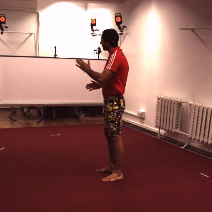

Acknowledgements

This thesis marks the final part of my 2-year master study at TU Delft, and it would not
have been possible without the supervision of Dr. Jens Kober and Dr. Osama Mazhar. Your
motivating guidance has in many ways shaped my attitude towards research.

   I would like to express my gratitude towards Shantanu Shivankar, Varun Kotian, Nikhil
Nagendra, and Lokin Prasad for their advice, company, and Indian food.
   My thanks extend to Vasileios Sfetsios, who provided warm company in this rather
tough and lonely times at the dormitory.
   I would not have developed such coding skills without constantly exchanging knowl-
edge with Asier Galicia Martínez.

   Many thanks to my parents for their unconditional and unequivocal support.

   Immense gratitude to Chia-Jou Chu for her continuous encouragement since my un-
dergraduate study in Japan.

                                                                           Yen-Lin Wu
                                                                Rotterdam, August 2021

                                           v

Contents

Abstract                                                                                                                                                              iii
Acknowledgements                                                                                                                                                       v
List of Figures                                                                                                                                                       ix
List of Tables                                                                                                                                                        xi
Nomenclature                                                                                                                                                         xiii
1 Introduction                                                                                                                                                         1
2 Related Works                                                                                                                                                        3
   2.1 2D human pose estimation          .   .   .   .   .   .   .   .   .   .   .   .   .   .   .   .   .   .   .   .   .   .   .   .   .   .   .   .   .   .   .     3
   2.2 3D human pose estimation          .   .   .   .   .   .   .   .   .   .   .   .   .   .   .   .   .   .   .   .   .   .   .   .   .   .   .   .   .   .   .     4
       2.2.1 Model-free . . . . . .      .   .   .   .   .   .   .   .   .   .   .   .   .   .   .   .   .   .   .   .   .   .   .   .   .   .   .   .   .   .   .     5
       2.2.2 Model-based . . . . .       .   .   .   .   .   .   .   .   .   .   .   .   .   .   .   .   .   .   .   .   .   .   .   .   .   .   .   .   .   .   .     6
   2.3 Evaluation metrics . . . . .      .   .   .   .   .   .   .   .   .   .   .   .   .   .   .   .   .   .   .   .   .   .   .   .   .   .   .   .   .   .   .     7
   2.4 Kinematic constraints . . .       .   .   .   .   .   .   .   .   .   .   .   .   .   .   .   .   .   .   .   .   .   .   .   .   .   .   .   .   .   .   .     9
   2.5 Deep rotation estimation .        .   .   .   .   .   .   .   .   .   .   .   .   .   .   .   .   .   .   .   .   .   .   .   .   .   .   .   .   .   .   .     9
   2.6 Transformer-based works .         .   .   .   .   .   .   .   .   .   .   .   .   .   .   .   .   .   .   .   .   .   .   .   .   .   .   .   .   .   .   .    10

3 Joint Detection Approach                                                                                                                                            11
   3.1 What is Transformer? . . . . .        .   .   .   .   .   .   .   .   .   .   .   .   .   .   .   .   .   .   .   .   .   .   .   .   .   .   .   .   .   .    11
       3.1.1 Embeddings . . . . . .          .   .   .   .   .   .   .   .   .   .   .   .   .   .   .   .   .   .   .   .   .   .   .   .   .   .   .   .   .   .    11
       3.1.2 Positional encoding. .          .   .   .   .   .   .   .   .   .   .   .   .   .   .   .   .   .   .   .   .   .   .   .   .   .   .   .   .   .   .    12
       3.1.3 Multi-head attention .          .   .   .   .   .   .   .   .   .   .   .   .   .   .   .   .   .   .   .   .   .   .   .   .   .   .   .   .   .   .    13
       3.1.4 Encoder . . . . . . . . .       .   .   .   .   .   .   .   .   .   .   .   .   .   .   .   .   .   .   .   .   .   .   .   .   .   .   .   .   .   .    13
       3.1.5 Decoder. . . . . . . . .        .   .   .   .   .   .   .   .   .   .   .   .   .   .   .   .   .   .   .   .   .   .   .   .   .   .   .   .   .   .    13
   3.2 Architecture of PETR . . . . .        .   .   .   .   .   .   .   .   .   .   .   .   .   .   .   .   .   .   .   .   .   .   .   .   .   .   .   .   .   .    14
   3.3 Dataset preprocessing . . . .         .   .   .   .   .   .   .   .   .   .   .   .   .   .   .   .   .   .   .   .   .   .   .   .   .   .   .   .   .   .    15

4 Kinematic Model Approach                                                                                                                                            17
   4.1 Architecture of PEBRT . . . . . . . . . . . . . . .                               .   .   .   .   .   .   .   .   .   .   .   .   .   .   .   .   .   .   .    17
   4.2 Human Kinematic model . . . . . . . . . . . . .                                   .   .   .   .   .   .   .   .   .   .   .   .   .   .   .   .   .   .   .    18
   4.3 Rotation estimation . . . . . . . . . . . . . . . . .                             .   .   .   .   .   .   .   .   .   .   .   .   .   .   .   .   .   .   .    19
       4.3.1 Recovering rotation matrix . . . . . . . .                                  .   .   .   .   .   .   .   .   .   .   .   .   .   .   .   .   .   .   .    19
       4.3.2 Obtaining ground-truth rotation matrix                                      .   .   .   .   .   .   .   .   .   .   .   .   .   .   .   .   .   .   .    20
       4.3.3 Verifying implementation . . . . . . . . .                                  .   .   .   .   .   .   .   .   .   .   .   .   .   .   .   .   .   .   .    21
   4.4 Loss function . . . . . . . . . . . . . . . . . . . . .                           .   .   .   .   .   .   .   .   .   .   .   .   .   .   .   .   .   .   .    22
   4.5 Novel evaluation metric . . . . . . . . . . . . . .                               .   .   .   .   .   .   .   .   .   .   .   .   .   .   .   .   .   .   .    23
   4.6 Additional loss term. . . . . . . . . . . . . . . . .                             .   .   .   .   .   .   .   .   .   .   .   .   .   .   .   .   .   .   .    24

                                                             vii
viii                                                                                                                                 Contents

5 Experimental Setup                                                                                                                             27
       5.1 Implementation details . . . . . . . . . . . . . .        .   .   .   .   .   .   .   .   .   .   .   .   .   .   .   .   .   .   .   27
       5.2 Experiment results . . . . . . . . . . . . . . . . .      .   .   .   .   .   .   .   .   .   .   .   .   .   .   .   .   .   .   .   28
           5.2.1 Discussion on PETR . . . . . . . . . . . .          .   .   .   .   .   .   .   .   .   .   .   .   .   .   .   .   .   .   .   28
           5.2.2 Discussion on PEBRT. . . . . . . . . . . .          .   .   .   .   .   .   .   .   .   .   .   .   .   .   .   .   .   .   .   28
           5.2.3 Comparison between PETR and PEBRT.                  .   .   .   .   .   .   .   .   .   .   .   .   .   .   .   .   .   .   .   29
           5.2.4 Results with additional loss term. . . . .          .   .   .   .   .   .   .   .   .   .   .   .   .   .   .   .   .   .   .   30
       5.3 Qualitative results . . . . . . . . . . . . . . . . . .   .   .   .   .   .   .   .   .   .   .   .   .   .   .   .   .   .   .   .   31
           5.3.1 PETR . . . . . . . . . . . . . . . . . . . . .      .   .   .   .   .   .   .   .   .   .   .   .   .   .   .   .   .   .   .   31
           5.3.2 PEBRT . . . . . . . . . . . . . . . . . . . . .     .   .   .   .   .   .   .   .   .   .   .   .   .   .   .   .   .   .   .   33
       5.4 Further Improvements . . . . . . . . . . . . . . .        .   .   .   .   .   .   .   .   .   .   .   .   .   .   .   .   .   .   .   35
6 Conclusion                                                                                                                                     37
Bibliography                                                                                                                                     39
List of Figures
1.1 An example of kinematically unrealistic output . . . . . . . . . . . . . . . . . . 2
2.1 Illustration of commonly used 2D estimators . . . . . . . . . . . . . . . . . . . 3
2.2 Example input and output of HRNet . . . . . . . . . . . . . . . . . . . . . . . . . 4
2.3 Model-free 3D human pose estimation . . . . . . . . . . . . . . . . . . . . . . . 5
2.4 Human body models . . . . . . . . . . . . . . . . . . . . . . . . . . . . . . . . . . 6
3.1 Transformer model architecture . . . . . . . . . . . . . . . . . . . . . . . . . . . 12
3.2 Visualization of positional encoding . . . . . . . . . . . . . . . . . . . . . . . . . 13
3.3 Multi-head attention . . . . . . . . . . . . . . . . . . . . . . . . . . . . . . . . . . 14
3.4 Architecture of PETR . . . . . . . . . . . . . . . . . . . . . . . . . . . . . . . . . . 14
3.5 Joints order . . . . . . . . . . . . . . . . . . . . . . . . . . . . . . . . . . . . . . . . 15
4.1 Architecture of PEBRT . . . . . . . . . . . . . . . . . . . . . . . . . . . . . . . . . 17
4.2 An overview of PEBRT pipeline . . . . . . . . . . . . . . . . . . . . . . . . . . . . 18
4.3 Human kinematic model . . . . . . . . . . . . . . . . . . . . . . . . . . . . . . . 19
4.5 An example of imposing GT information on our human model . . . . . . . . . 21
4.6 Illustration of MAEV . . . . . . . . . . . . . . . . . . . . . . . . . . . . . . . . . . 22
4.7 Preprocessing 3D keypoints . . . . . . . . . . . . . . . . . . . . . . . . . . . . . . 23
4.8 Mismatched camera angle . . . . . . . . . . . . . . . . . . . . . . . . . . . . . . . 24
4.9 Including projected 2D keypoints for training . . . . . . . . . . . . . . . . . . . 25
5.1 Results comparison in "SittingDown" by PETR and PEBRT . . . . . . . . . . . . 30
5.2 Qualitative results on Human3.6M by PETR . . . . . . . . . . . . . . . . . . . . 31
5.3 Qualitative results on MPI-INF-3DHP by PETR . . . . . . . . . . . . . . . . . . 32
5.4 Qualitative results on Human3.6M by PEBRT . . . . . . . . . . . . . . . . . . . . 33
5.5 Qualitative results on Human3.6M by PEBRT . . . . . . . . . . . . . . . . . . . . 34
ixList of Tables
2.1 Average 3D Reconstruction error on Human3.6M in Protocol 1 (mm) . . . . . 8
2.2 3D reconstruction error on MPI-INF-3DHP in 3DPCK (%) . . . . . . . . . . . . 8
4.1 Body segment lengths and joint constraints . . . . . . . . . . . . . . . . . . . . 19
5.1 Number of parameters given different layers of Transformer encoder . . . . . 27
5.2 3D Reconstruction error on Human3.6M reported in MPJPE 1 . . . . . . . . . 28
5.3 Reconstruction error on Human3.6M reported in MPBVE . . . . . . . . . . . . 29
5.4 Comparison between PETR and PEBRT on Human3.6M in MPJPE . . . . . . . 29
5.5 Additional attempts to improve model accuracy . . . . . . . . . . . . . . . . . . 30
xiNomenclature
Abbreviations
M P BV E Mean Per Bone Vector Error
M P J PE Mean Per Joint Position Error
PC K Percentage of Correct Keypoints
SM P L Skinned Multi-Person Linear
SV D Singular Value Decomposition
Symbols
α Yaw
β Pitch
γ Roll
B̂i Normalized bone vector of i − bone
Boi Bone vector of i −th bone of a T-pose
Bi Bone vector of i −th bone
E Extrinsic camera matrix
J Joint coordinates
K Intrinsic camera matrix
R∗i GT Rotation matrix of i −th bone
p
Ri Rotation matrix of i −th bone from projected 2D inputs
Ri Rotation matrix of i −th bone
wpuni sh Array of punishing weights
Bt Total number of bones
dk Dimension of Key
d mod el Dimension of model
Jt Total number of joints
xiiixiv Nomenclature K Key N Number of Encoder layers Q Query V Value
1
                                                                Introduction

Human pose estimation (HPE) has long captivated the attention of researchers in Com-
puter Vision. It is a study of estimating human body configuration from a single image or
video, whose application encompasses action recognition [33, 42], human-robot interac-
tion [62, 86], autonomous vehicle [20], surveillance [23], and avatar generation [29].

   Recent works have leveraged the power of Convolutional Neural Network (CNN) to
achieve 2D human pose estimation [5, 11, 49] from RGB images. In contrast, 3D human
pose estimation is a much more difficult task due to limited dataset available and depth
ambiguities. Also, body configuration includes high degree-of-freedom joints, resulting in
high-dimensional solution space. Occlusion and truncation can lead to temporal inco-
herency in pose estimation. Rare and complex poses (e.g. yoga and extreme sports) may
be more difficult to infer.

    Modern works take 3D pose estimation as a coordinate regression problem, which ne-
glects the human body kinematics and often leads to unrealistic results. In other words.,
they only regress the coordinates of body joints and does not take account of the structured
dependency between keypoints. An example is shown in Figure 1.1. Sun et al. [65] define
a compositional loss function that encodes local bone relationships. Wandt et al. [73] pro-
pose Kinematic Chain Space (KCS) matrix that asserts consistent bone lengths throughout
the entire image sequence. However, accurate MoCap system and prior knowledge (e.g.
bone length) on the human object are required. Dabral et al. [15] introduce illegal angle
loss and symmetry loss to model joint relationship of human pose. Illegal angle loss is lim-
ited to only elbow and knee joints since 2 parent links are required to calculate a normal
vector whose dot product with lower arm or calf is positive. Xu et al. [79] conduct pose
refinement on unreliably estimated joints using motion trajectory of a child joint relative
to parent joint. This approach is, again, built upon the assumption of accurate MoCap sys-
tem and is subject to noisy inputs. On top of that, the above methods of adding additional
loss terms may help achieve better accuracy but still does not guarantee realistic final 3D
outputs. This prohibits the application in simulation environments and avatar control.

                                             1
2 1. Introduction
Figure 1.1: An example of kinematically unrealistic output.
Red circle: left lower arm does not have the same length with right counterpart;
cyan circle: knee joint has a unrealistic rotation to the right.
As Zheng et al. [83] point out, angle representation is pose-dependent and does not
concern body shape. For example, we consider a ROS simulation scenario where con-
trolling a fix-sized Urdf model takes place. Accurate and realistic pose information is a
prerequisite to simulation applications. However, pure joint detection struggles to map
a single pose to different avatars as every human skeleton has different shape, hence dif-
ferent joint positions. Designing a pipeline that can digest pose information regardless of
object’s height or shape and guarantees kinematically realistic outputs is a less researched
and overlooked topic.
We are motivated to introduce a human kinematic model that is encapsulated with
bone length and joint angle constraints. In this work, we incorporate a human kinematic
model into deep models that regresses rotation matrix parameters for each bone. We pro-
pose "Pose Estimation via Bone Rotation using Transformer (PEBRT)" for monocular 3D
human pose estimation. It is a regression approach using a rotation-based representation
that incorporates human pose structure. Specifically, our contributions in this work are as
follows:
• Our framework does not require receptive field, i.e. multi-frame inputs, to achieve
comparable results to existing methods
• Our pipeline recovers rotation matrices from network output and impose them on a
kinematic human model
• We propose a new metric that evaluates pose accuracy regardless of human body
shape, gender, or age.
To our knowledge, this is the first attempt to formulate human pose estimation with a
kinematic model and focus on bone rotations in the entire pipeline. We conduct ablation
study to compare the performance on different number of layers of Transformer Encoder.
Further experiments show that our model achieve comparable performance to state-of-
the-art methods on two widely used 3D human motion datasets.2
Related Works
This chapter aims to provide a solid ground to the motivation behind our research question
by covering 2D and 3D HPE, rotation analysis, and Transformer-based works. Strengths
and weaknesses of various 3D HPE methods are also discussed.
2.1. 2D human pose estimation
Accurate 2D estimation is regarded as the prerequisite for accurate 3D prediction. Figure
2.1 is an illustration of commonly used 2D estimators in 3D human pose estimation. De-
tails of each method are given in the next paragraph.
Figure 2.1: Illustration of commonly used 2D estimators [64].
(a) Hourglass [49]; (b) Cascaded pyramid networks [11]; (c) Simple Baseline [77]; (d) HRNet [64].
34 2. Related Works
(a): Newell et al. [49] introduce repeated conv-deconv modules named Stacked Hour-
glass Network (SHN). Through iterative refinement with residual connections in between,
spatial information can be preserved and each joint can be localized.
(b): Chen et al. [11] propose Cascaded Pyramid Network (CPN) for multi-person pose
estimation that consists of two sub-networks, GlobalNet and RefineNet. GlobalNet directly
recognizes "easy" keypoints from generated heatmaps, whereas RefineNet explicitly ad-
dresses the "hard" keypoints based on an exclusive loss.
(c): Transposed convolution layers were adopted in Simple Baseline [77] to generate
high-resolution representations.
(d): In contrast to SHN, Sun et al. [64] introduce High-Resolution Net (HRNet) that
maintains high-resolution representations throughout the network and aggregates infor-
mation from parallel sub-networks.
The High-Resolution Network (HRNet) [64] contains 4 convolutional layers and assumes
a 256x256 image as input. The output is J t heatmaps, corresponding to each of the J t joints.
This architecture is used in the pilot implementation of this work as a baseline. It aims to
serve as a CNN backbone that extracts 2D keypoints from RGB images.
Figure 2.2: An example input and output from HRNet [64].
Left: a RGB image input; right: stacked heatmap corresponding to 17 human joints
2.2. 3D human pose estimation
Some 3D HPE works took advantage of multi-camera settings [19, 27] or depth sensors
[56, 62, 86] to achieve accurate estimations. However, such specialized setups are not avail-
able to general public, major focus has shifted to developing frameworks for monocular 3D
human pose estimation. This section divides deep learning-based 3D HPE methods into 2
categories: model-free and model-based human pose estimation. As mentioned in Chap-
ter 1, predicting depth information from 2D images is an under-constrained task. While
training on a model-free architecture is easier, invalid or unrealistic poses can be expected.
With kinematic constraints or a reference structure, outputs are guaranteed to have plausi-
ble poses. It can, however, take a toll on 3D pose inference time and computing efficiency
depending on the optimization approach.2.2. 3D human pose estimation 5
2.2.1. Model-free
Figure 2.3: Model-free 3D human pose estimation.
Red arrow: Single-stage method; blue arrow: 2D-3D lifting method
Model-free methods can be divided into 2 groups:
1) Direction 3D regression [52, 53, 66], or single-stage methods, skips any intermediate
prediction and outputs 3D poses given an RGB image/video as input. The training of such
model is easier than 2D-3D lifting while lacking intermediate constraints.
Kanazawa et al. [29], Zheng et al. [83], and Arnab et al. [2] argue that information ex-
tracted from images is not leveraged for depth inferences. 2D-3D lifting models can depend
solely on input 2D keypoints, thus limiting the final performance. Some of these methods
also model 2D-3D correspondences from dataset. As mentioned by Chen et al. [9], they
incorporate dataset-specific parameters (e.g. camera projection matrix, scale of skeleton,
object distance to camera) and achieve good accuracy. However, their performance on in-
the-wild image/video would be questionable. Arnab et al. [2] reason that overfitting to
constrained lab environment is a concern that prevents the model from generalizing well
to real-world images.
Pavlakos et al. [52] is an example of direction 3D pose estimation. The network predicts
per voxel likelihoods for each joint and through repetitive processing and refinement it out-
puts a final 3D pose. Sun et al. [66] argue that heatmap representation is non-differentiable
and thus cannot be backpropagated. They propose Integral Pose Regression method to
transform heatmaps into joint location coordinate, which is differentiable and in turn al-
lows end-to-end training.
2) 2D-3D lifting [8, 44, 48, 60, 67, 71] is also called two-step/-stage pose estimation. It
breaks down the estimation process into: i. Producing accurate 2D poses using off-the-
shelf 2D pose estimator (e.g. SHN, CPN). ii. Lifting the 2D joints to 3D by predicting their
respective depth. One of its advantage is that 2D dataset can also be used for training. Chen
et al. [9] and Wandt et al. [73] project 3D predictions back to 2D image space and calculate
loss.6 2. Related Works
2D-3D lifting is an inherently ill-posed problem. While 2D-3D lifting methods some-
times show better performance than the direct regression ones (see Table 2.1, 2.2), their
overall accuracy and inference time are dependent and bottlenecked by the 2D estimator.
2D-3D lifting methods can be trained on 2D dataset by projecting 3D poses to 2D image
space [47], whereas direct regression methods depend on synthetic data if more training
data is required [46].
Chen et al. [8] and Rogez et al. [60] do not depend on the 2D estimator alone but cre-
ate a pose library for matching purpose. Chen et al. [8] set up a library of 200,000 poses
and performed k nearest neighbor search to estimate 3D pose from 2D keypoints. In [60],
they pre-process a fixed set of 2D-3D anchor-poses and estimate respective probability to
be correct at each location. They perform pose proposal integration (PPI) to aggregate pro-
posals that are close in terms of image location and 3D pose. However, both their per-
formances are limited by the pose library size. Computation speed also depends on the
matching algorithm and library size.
Martinez et al. [44] is the first one to use deep neural network to realize the concept
of lifting 2D to 3D. The lightweight model in [44] set a baseline in the "lifting" category.
Veges and Lorincz [71] employ energy optimization based smoothing method to adaptively
smoothen 3D poses such that temporarily invisible human does not undermine estimation
results. Pavllo et al. [55] implement dilated temporal convolutions and receptive fields to
capture long-term information.
2.2.2. Model-based
Model-based approaches come in different forms of representation based on the detail
and attribute to describe human body shape. Kinematic models output human pose or
skeleton, whereas volumetric models provide more information regarding body shape by
rendering meshes. Figure 2.4 shows an example of commonly used human models in 3D
human pose estimation.
Figure 2.4: Human body models [12]:
(a) Kinematic model; (b) volumetric model2.3. Evaluation metrics 7
Kinematic model: Kinematic models, also known as skeleton-based models, contain
a set of joints locations and their corresponding limb orientations. Constraints on bone
length or joint angles can thus be applied to such model. Their simple topology makes
them popular among researchers, used in [13, 47, 50, 73]. However, kinematic models fall
short of texture or shape information.
Nie et al. [50] employ a two-level LSTM architecture to regress depth element for each
joint. The first level captures 2D poses from corresponding image patches and human
skeletons from 3D pose library, while the second level integrates both global and local fea-
tures to predict joint depth. Mehta et al. [47] is the first to achieve real-time 3D single hu-
man pose estimation from a single RGB camera following kinematic skeleton fitting. Their
method was claimed to outperform RGB-D cameras (e.g. Kinect [22]) in outdoor scenarios.
Volumetric model: There has been extensive research [2, 3, 40, 54, 69] in human body
shape rendering in deep-learning based methods. One of the most widely employed model
is Skinned Multi-Person Linear (SMPL) model, introduced by Loper et al. [40] and renders
a wide range of human body shape using a statistical parametric function, 6890 vertices,
and 23 joints.
Pavlakos et al. [54] directly predict SMPL parameters given 2D joints and silhouettes.
Tripathi et al. [69] employ knowledge distillation and trained student network exclusively
for SMPL body parameter prediction. Similarly, Arnab et al. [2] take advantage of adver-
sarial learning to produce more human models, after which an additional discriminator
network distinguishes real models.
2.3. Evaluation metrics
Human3.6M [28] is the most widely used indoor dataset for single person 3D HPE. It con-
tains 3.6 million different human poses collected with 4 digital cameras and consists of
11 professional actors (6 male and 5 female) with different BMI. The actors performed 15
different daily tasks such as walking, smoking, talking on the phone, etc. Provided annota-
tions include 3D joint positions, joint angles, person bounding boxes, and 3D laser scan of
each actor Evaluation results are reported in Mean Per Joint Position Error (MPJPE), also
known as reconstruction error or 3D error, is the most widely used metric found in liter-
ature. It calculates the Euclidean distance from estimated 3D joints to ground truth and
average over all joints. It can be written in the form of Equation 2.1.
1 X J
M P J PE = ||Ji − J∗i ||2 (2.1)
J t i =1
, where J t is the total number of joints, Ji and J∗i stand for estimated and ground truth
position of joint i . This measurement is reported in millimeters (mm) in 3D or pixel in 2D.
MPJPE is considered a generalized baseline metric since it adapts to different dataset that
have different number of keypoints. Methods using root-relative pose or absolute pose can
be measured using MPJPE. In Human3.6M protocol 1, MPJPE is calculated after aligning
the depth of root joint; protocol 2 and 3 is the MPJPE after a rigid transformation using
Procrustes Analysis, called P-MPJPE or Reconstruction Error.8 2. Related Works
MPI-INF-3DHP [45] contains 8 subjects (4 male and 4 female) performing 8 activities,
ranging from walking, sitting, sports, etc. There are a total of 1.3 million frames from 14
different angles. They are captured using markerless MoCap system in green screen back-
ground, which allows data augmentation such as chroma key compositing.
Percentage of Correct Keypoints (PCK) & Area Under Curve (AUC) are suggested by
Mehta et al. [45] for more expressive and robust 3D HPE evaluation. AUC is tasked to com-
pute a range of PCK thresholds. Whereas PCK/3DPCK considers a detected joint correct if
its distance to ground-truth joint is within a certain threshold, where the default value is
150mm. Our models are only evaluated on Human3.6M in this work in MPJPE.
Table 2.1: Average 3D Reconstruction error on Human3.6M in Protocol 1 (mm)
Method Input Backbone MPJPE ↓
Model-free
Chen et al. [8] CVPR’17 2D CPN 82.7
Pavlakos et al. [52] CVPR’17 Image SHN 71.9
Tekin et al. [67] ICCV’17 Image SHN 69.7
Matrinez et al. [44] ICCV’17 Image SHN 62.9
Pavlakos et al. [53] CVPR’18 Image SHN 56.2
Sun et al. [66] ECCV’18 Image ResNet, SHN 49.6
Pavllo et al. [55] CVPR’19 2D CPN 46.8
Model-based
Mehta et al. [47] SIGGRAPH’17 Image ResNet 80.5
Nie et al. [50] ICCV’17 Image LSTM 79.5
Wandt et al. [72] ECCV’18 Image - 89.9
Cheng et al. [13] AAAI’20 Image HRNet 40.1
Chen et al. [10] TCSVT’21 2D CPN 44.1
Table 2.2: 3D reconstruction error on MPI-INF-3DHP in 3DPCK (%)
Method Input Backbone 3DPCK ↑
Model-free
Matrinez et al. [44] ICCV’17 2D SHN 68.0
Pavlakos et al. [53] CVPR’18 Image SHN 71.9
Pavllo et al. [55] CVPR’19 2D CPN 86.0
Model-based
Mehta et al. [47] SIGGRAPH’17 Image ResNet 79.4
Wandt et al. [72] CVPR’19 Image - 82.5
Cheng et al. [13] AAAI’20 Image HRNet 84.1
Veges and Lorincz [71] ICONIP’20 2D - 85.3
Chen et al. [10] TCSVT’21 2D CPN 87.92.4. Kinematic constraints 9
2.4. Kinematic constraints
Several works apply previously learnt properties to guarantee valid and realistic 3D poses.
Anthropometric priors include bone lengths [13, 59, 73], limb proportions [74], or joint
angle constraints [1, 83].
Sun et al. [65] address the problem using a regression-based method, instead of pure
joint detection. Dabral et al. [15] introduce illegal angle loss and symmetry loss to model
joint relationship of human pose. Wandt et al. [73] propose Kinematic Chain Space (KCS)
matrix that implicitly models the kinematic chain of human skeletons without motion pri-
ors. The KCS matrix makes it easier to impose constraints on bone length and joint angle.
Cheng et al. [72] extend the concept in [73] to a temporal application- TKCS, that reports
the change in length and angle across different frames in a video. In other words, TKCS en-
sures the spatial and temporal validity of 3D poses. Zheng et al. [83] introduce joint angle
prediction constraint in their loss function.
While these methods are able to produce competitive results in accuracy, they assert
accurate data input prior knowledge (such as bone length) on the human object. Also,
additional terms in loss function does not guarantee realistic final 3D outputs. We design
a kinematic human model that contain bone length and joint angle constraints as a novel
approach to 3D human pose estimation.
2.5. Deep rotation estimation
There has been prevalent research on rotation estimation, with the output being one of the
followings: Euler angles, quaternions, axis-angles, or rotation matrix parameters.
Both Euler angles and quaternions have their limitations in 3D rotation representations,
making them difficult for deep neural network to learn [61, 85]. Euler angle representation
for 3D rotation shows discontinuity in the case of identity rotation I, i.e. θ can either be 0
or 2π. A common issue with Euler angle (α, β, γ) that causes ambiguity is known as gimbal
lock [30]. This occurs when two rotating axes become parallel, one degree of freedom is
lost. The order of rotating axis also needs to be specified in advance. Saxena et al. [61]
point out that a quaternion q = (q x , q y , q z , q w ) has the antipodal problem, resulting in q
and −q to have the same rotation. The axis-angle representation (α, θ) is computationally
inefficient in terms of its rotation compositions.
Fisch and Clark [21] propose a 12D over-parameterization called orientation keypoints
that model both translation and rotation. However, roll angles are not always available in
public dataset, e.g. MPI-INF-3DHP [45]. Zhou et al. [85] mathematically prove that such
discontinuity and ambiguity stem from 3D rotation representation with 4 or lower dimen-
sions. They further propose general rotation representations by performing Gram-Schmidt
orthogonalization. Specifically, they present a continuous n 2 − n dimensional representa-
tion for the n dimensional rotation group SO(n). In this work, we utilize this general repre-
sentation to recover rotation matrices for each bone in the human model.10 2. Related Works
Another attempt to recover a rotation matrix is by Levinson et al. [32], who implement
symmetric orthogonalization via Singular Value Decomposition (SVD) on neural network
outputs. Cao et al. apply such SVD orthogonalization to recover rotation matrices in the
study of head pose estimation. Their work also introduce a novel loss function called Mean
Absolute Error on Vectors (MAEV). We borrow and modify MAEV to use it as our loss func-
tion in our framework.
The above studies in rotation estimation has been widely adopted in 6D object pose
estimation and structure from motion (SfM), where the orientation of a single object is
estimated. While in human pose estimation, there has not been works estimating bone
rotation in the framework. In this paper, we propose a novel approach to estimate the
orientation for multiple bones in the human skeleton.
2.6. Transformer-based works
With the introduction of self-attention mechanisms, Liu et al. [38] reason that it cap-
tures long-range temporal relationships and brings temporal coherency to pose prediction.
Since the introduction of Transformer [70], it has stirred up immense interest accompanied
with significant progress in language understanding [16, 39, 57] and in image understand-
ing tasks [7, 17, 51, 58, 68].
There has been several attempts to implement Transformer for pose estimation [34, 35,
43, 80, 82]. Zheng et al. [82] use a ViT-based architecture to capture spatial and temporal
information to lift 2D keypoints to 3D pose. Lin et al. [35] combine CNN with Transformer
Encoder to output human body meshes. Mao et al. [43] propose a regression-based ap-
proach which avoids the feature misalignment issue. Li et al. [34] employ full encoder-
decoder Transformer architecture to perform keypoint/joint regression.
Given its successful implementation on image understanding tasks [7, 17, 36, 75], we
are curious about Transformer’s potential in handling sequences such as joint coordinates.
Though Transformer has demonstrated improved training speed, its inference time strug-
gles to keep up due to its auto-regressive schema in the decoder [81]. Xu et al. [78] acquire
faster inference time using Transformer by discarding decoder layers. In this work, we use
only the encoder part of Transformer with its potential real-time application in mind.3
Joint Detection Approach
Following the majority of research in human pose estimation, we propose an end-to-end
2D-3D lifting approach for 3D human pose estimation. We employ HRNet as the feature
extractor, followed by Transformer Encoders and a fully-connected (FC) layer. This section
introduces the cutting-edge model Transformer, camera projection needed to process the
dataset, and the architecture of our pilot implementation on human pose estimation.
3.1. What is Transformer?
Sequence-to-sequence (Seq2Seq) problems, such as language modeling and neural ma-
chine translation, used to be tackled with Recurrent Neural Network (RNN) and Long Short-
Term Memory (LSTM). However, their applications are not without limitations. They strug-
gle with long sequence input since the reference window limits how far they can look back
in the input. Physical memory constraints also act as a setback against long sequence in-
put. This results in vanishing gradient as important information is forgotten after layers
and layers of training.
This section introduces the cutting-edge technique proposed by Vaswani et al. [70],
known for its robust performance in Natural Language Processing (NLP). The working prin-
ciple of Transformer and its application in Computer Vision, especially in HPE, will be dis-
cussed by introducing state-of-the-art research. [70] address the input sequence limit by
introducing a model that depends entirely on attention mechanism, dispensing convolu-
tion and recurrence. Transformer follows this overall architecture (Figure 3.1) using multi-
head attention and point-wise, fully connected layers for both encoder and decoder.
3.1.1. Embeddings
Before feeding a word sequence into Transformer, words need to be converted to vectors
for the computer to understand. Word embeddings are regarded as dense representations
where words with similar meanings are close to each other and have similar vector repre-
sentations.
1112 3. Joint Detection Approach
Figure 3.1: Transformer model architecture [70]
3.1.2. Positional encoding
Due to absence of recurrence and convolution, information of relative or absolute posi-
tion of the token needs to be embedded for Transformer. Without positional information,
"Kevin hurt the dog" would have the same representation as "the dog hurt Kevin". [70]
use simple si n and cos function to generate positional encoding, as shown in Equation
(3.1),(3.2), where pos and i stand for the position and dimension, and d mod el is the model
dimension. The amplitude of the encoding is bounded by −1 and 1 thanks to the trigono-
metric functions.
Figure 3.2 is a visualization of the positional encoding used in [70]. We inherit the orig-
inal implementation in this work. The encoded value are added to the vector representa-
tion, allowing us to distinguish the order.
PE (pos,2i ) = si n(pos/100002i /dmod el ) (3.1)
PE (pos,2i +1) = cos(pos/100002i /dmod el ) (3.2)3.1. What is Transformer? 13
Figure 3.2: Visualization of positional encoding
3.1.3. Multi-head attention
Transformer adopts scaled dot-product attention, as shown in Equation (3.3). The output
is a weighted sum of values (V ), whose weight is obtained by the dot-product of the query
(Q) with all the keys (K ).
QK T
At t ent i on(Q, K ,V ) = so f t max( p )V (3.3)
dk
where Q, K, V are matrices for queries, keys, and values, d k is the dimension of K , and p1
dk
serves as a scaling factor.
For each single word in the sequence, self-attention generates an attention vector that
models its contextual relationship with all other words in the same sequence. This not
only solves the long-range dependency issues that RNN faced with, but also works under
parallelization, making it more computationally efficient 1 than convolution and recursive
operations. This brings us to the definition of multi-head attention, where attention layers
are stacked in parallel.
3.1.4. Encoder
Each encoder block includes a multi-head attention and a feed-forward layer. The multi-
head attention layers outputs multiple attention vectors. The feed-forward layer is tasked
to convert them into a single attention vector by normalization for the succeeding encoder
or decoder block to process. A total number of 6 layers of encoder was used in [70]. We
conduct ablation studies on layer numbers of encoder in this work.
3.1.5. Decoder
The masked multi-head attention generates attention vectors for each word in the output
sequence. Instead of using every element like encoder does, the masked multi-attention
can only refer to previous outputs. Any future elements are masked by setting their values
to zero. In the next attention layer, we have output from the last encoder transformed into
1
Table 1 of [70] gives computing complexity of convolutional, recurrent, and self-attention model.14 3. Joint Detection Approach
Figure 3.3: Multi-head attention [70] stacks h layers of scaled dot-product attention in parallel before con-
catenating their attention scores
matrix K and V , with Q being the output from masked multi-head attention. This is the
process where the relationship between input and output sequence are mapped.
Similar to encoder, multiple attention vectors are normalized to a single one. [70] use 6
layers of decoder before output to the final linear layer.
3.2. Architecture of PETR
Our first model follows an end-to-end approach- inferring 3D keypoints directly from a
monocular image. The HRNet takes in an RGB image and outputs 17 heatmaps, each high-
lights a different joint location. By unraveling the index, the 2D coordinates of each joint
can be obtained, giving us an array of (17,2). Transformer encoder assumes concatenated
(x,y) coordinates of the 17 joints that are added with positional encoding. The output of
encoder gives us the same shape of array, (1,34). Finally, the fully-connected (FC) layer and
t anh activation function outputs a prediction of the 3D pose. Figure 3.4 shows an instan-
tiation of our architecture.
Figure 3.4: Architecture of PETR.
The pipeline accepts RGB image as input, generates a heatmap of human joints, feed them into N layers of
Transformer Encoders followed by a linear layer and a t anh activation function, and outputs a single 3D pose.3.3. Dataset preprocessing 15
Xu et al. [78] investigate the effect on the number of encoder and decoder layer in word
translation tasks. Their experiments show that trading decoder for encoder layers accom-
panies marginal loss in accuracy, less number of parameters, and more than 3 times faster
inference time. We only make use of the encoder part of Transformer due to the concern of
inference speed.
3.3. Dataset preprocessing
We standardize the dataset before using since they 1) come in different joints order, and 2)
are captured in world coordinates. The output from pre-trained HRNet is in COCO format;
whereas Human3.6M [28] and MPI-INF-3DHP [45] comes in different order. We rearrange
and follow the joints order shown in Figure 3.5.
Figure 3.5: Joints order
(1. manubrium, i.e. midpoint of left and right clavicles; 2. mid-spine; 3. root; 4. neck; 5. face; 6. left shoulder;
7. left elbow; 8. left wrist; 9. right shoulder; 10. right elbow; 11. right wrist; 12. left hip; 13. left knee; 14. left
ankle; 15. right hip; 16. right knee; 17. right ankle)
Since intrinsic matrix is available in the majority of commercialized cameras, we pro-
cess 3D keypoints in camera coordinates, instead of in world coordinates. The advantage
is that the neural network will not predict the extrinsic matrix, which is unknown without
inference, and focus only on joint detection.
The 3D annotations in Human3.6M and MPI-INF-3DHP are given in world coordinates.
For the Human3.6M dataset, we borrow the processed file used in VideoPose3D [55]. It
includes 2D keypoints in pixel coordinates and 3D keypoints in camera coordinates, where
the root joint is centered at origin (0, 0, 0).16 3. Joint Detection Approach
On the other hand, 3D keypoints in MPI-INF-3DHP have to be manually projected.
Since intrinsic matrix are given, 3D keypoints in camera coordinates can be calculated.
The equation to relate 2D and 3D coordinates is given below:
x = PX (3.4)
X
u p1 p2 p3 p4
v = p 5 p 6 p 7 Y
p8 (3.5)
Z
1 p 9 p 10 p 11 p 12
1
, where x is a pixel coordinates (u, v) and X is a world coordinates (X , Y , Z ) in their homo-
geneous form, and P is a 3 × 4 camera matrix. Camera matrix P is commonly known as the
product of the intrinsic matrix K and extrinsic matrix E.
f s px r 1 r 2 r 3 t1
P = 0 f p y r 4 r 5 r 6 t2
0 0 1 r 7 r 8 r 9 t3 (3.6)
= K[R | t]
= KE
, where f is the camera focal length, (p x , p y ) is the principle point, s is the skew coefficient,
and R, t constitutes the extrinsic matrix , or rigid transformation, between world and cam-
era coordinate systems. Since it was found in [55] that the lens distortion has negligible
impact on the pose estimation metric, we assume 0 lens distortion in our work.
With the basic equations of camera projection and the method proposed by Lepetit et
al. [31], 3D keypoints in camera coordinates Xc can be recovered as follows.
Xc = EX = K−1 x (3.7)4
Kinematic Model Approach
This section addresses the architecture of Pose Estimation on Bone Rotation using Trans-
former (PEBRT). Instead of accurately detecting body joints from an image, we postulate
that pose estimation regardless of input skeleton size be the end goal. Hence in this sec-
tion, PEBRT is proposed to predict the rotation matrix parameters for each of the 16 bones
in a human body. The architecture inherits from PETR- Transformer encoders and a fully-
connected layer.
4.1. Architecture of PEBRT
With recent advent 2D joint detection methods such as Mask R-CNN [26] and CPN [11],
more research turns to 3D keypoints inference given 2D inputs. This model follows the
classic 2D-3D lifting approach that predicts root-relative 3D coordinates of joints associ-
ated to human skeletons. We use N layers of the original Transformer encoder, followed by
a linear layer and Tanh activation function that outputs B t ∗ 6 elements. This stands for
6 relevant elements of a rotation matrix of B t bones, to which the Gram-Schmidt process
[85] is applied to recover the rotation matrix for each bone. B t is 16 in our case.
Figure 4.1: Architecture of PEBRT.
The pipeline takes in a single 2D pose as input, feeds it through N layers of Transformer Encoders followed
by a linear layer. Gram-Schmidt process is applied to the linear layer output to recover rotation matrices for
each bone. The rotation matrices are applied to our human model for the final 3D pose.
1718 4. Kinematic Model Approach
Figure 4.2: An overview of PEBRT pipeline.
(1) Preprocess data to obtain GT rotation matrices for each bone. (2) The network outputs rotation matrices
during training. (3) Predicted rotation matrices can directly be applied to human model to make the pose.
An overview of PEBRT is shown in Figure 4.2. During data preprocessing in (1), a given
GT 3D pose is used to obtain rotation matrices for each bone taking T-pose as reference.
Gram-Schmidt process is applied to the network output, where the GT rotation matrices R∗i
are used to calculate MAEV loss [6] during training (2), where i stands for i −th bone. Finally
in (3), the predicted rotation matrices Ri are applied to a T-pose human model that rotates
each bone accordingly during inference. Details of each step are given in the following
sections.
4.2. Human Kinematic model
To create our novel kinematic model, we define the body segment lengths as given in [18]
and the joint range of motion as given in Appendix B of [25]. We follow the convention of
rotation whose yaw, pitch, roll are denoted by α, β, γ, respectively standing for rotation
about z−, y−, and x−axis. The human model is postured in T-pose by default (see Figure
4.3 (left)). We further define the bone vectors in the order shown in Figure 4.3 (right). The
information of parent/child bone to decide the punishing weight on each bone (see §4.4).
Table 4.1 gives the following information that is present in the model:
1. body segment lengths in a fraction of body height
2. joint constraints (in degrees) that are present in the model
3. whether each bone is categorized as a parent (P) bone or a child (C) bone
Note that the joint angles of a child bone is treated as relative rotation to its parent bone.4.3. Rotation estimation 19
Figure 4.3: Human kinematic model in 3D view (left) and the order of bone vectors (right)
(1. lower spine; 2. upper spine; 3. neck; 4. head; 5. left clavicle; 6. left upper arm; 7. left lower arm; 8. right
clavicle; 9. right upper arm; 10. right lower arm; 11. left pelvis; 12. left thigh; 13. left calf; 14. right pelvis; 15.
right thigh; 16. right calf)
Table 4.1: Body segment lengths in a fraction of body height H , joint constraints in Euler angles (deg), and
categories of parent (P) or child (C) bone
Body Part Length [αmi n , αmax ] [βmi n , βmax ] [γmi n , γmax ] P/C
Head 0.130H [-70,70] [-35, 35] [-55, 80] C
Neck 0.052H [0, 0] [0, 0] [0, 70] P
Upper spine 0.144H [0, 0] [0, 0] [0, 95] C
Lower spine 0.144H [-30, 35] [-35, 35] [-30, 75] P
Upper arm*2 0.186H [-45, 130] [-90, 130] [-90, 180] P
Lower arm*2 0.146H [0, 150] [0, 0] [0, 0] C
Thigh*2 0.245H [-45, 45] [-20, 50] [-30, 120] P
Calf*2 0.246H [0, 0] [0, 0] [0, 160] C
4.3. Rotation estimation
4.3.1. Recovering rotation matrix
Zhou et al. [85] suggest that functions of stronger continuity properties lead to lower ap-
proximation error. In other words, discontinuity hinders the performance of neural net-
works. They prove that 3D rotation representation is discontinuous in 4 or lower dimen-
sion, which indicates that it is inappropriate to use Euler angles or quaternion. Based on
the same argument, a 3D rotation matrix has 9 elements and thus do not have such discon-
tinuity issue.
A 3D rotation matrix is characterized as an orthogonal matrix with a determinant of +1.
All rotation matrices form a group called special orthogonal group SO(n), where n is the di-
mension. Levinson et al. [32] assume 9D network output, forming a noisy predicted matrix
R, and utilize SVD to find the the closest rotation matrix R̂. However, d et (R̂) is not guar-
anteed to be +1 depending on how noisy the original matrix is. [85] show a general form
of 3D rotation representation using Gram-Schmidt process with 6D overparameterization.
The mapping f GS from 6D representation to SO(3) can be obtained using Equation (4.1).20 4. Kinematic Model Approach
| | | | |
f GS a 1 a 2 = b 1 b 2 b 3 (4.1)
| | | | |
where
T
N (a 1 ) if i =1
b i = N (a 2 − (b 1 · a 2 )b 1 )
if i = 2
b1 × b2 if i =3
The 6D representation is beneficial to neural network since the Gram-Schmidt process
ensures the matrix orthogonality. It is a better approach than directly predicting 3x3 ro-
tation matrix since orthogonalization has to be done as a post-process, which has been
reported to have higher error [85] and also restricts applications in forward kinematics.
4.3.2. Obtaining ground-truth rotation matrix
In order to extract useful bone information, we use each ground-truth (GT) 3D pose and
a human model in T-pose to obtain the rotation matrix of each bone. In other words, we
calculate the rotation matrix R∗i that rotates i -th bone vector of T-pose Boi onto GT i -th
bone vector B∗i , i.e. B∗i = R∗i Boi . This idea is visualized in Figure 4.4.
Figure 4.4: Rotation matrices R∗i are obtained such that B∗i = R∗i Boi for i ∈ B t , where B∗i and Boi stand for the
i −th bone of GT pose and T-pose, and B t is total number of bones.
Essentially, we are calculating the rotation matrix that relates the two given vectors. Let
us first denote v = (v 1 , v 2 , v 3 ) = Boi × B∗i and c = Boi · B∗i . The rotation matrix R is given by
1−c
R = I + [v]× + [v]× (4.2)
s2
0 −v 3 v 2
[v]× := v 3 0 −v 1 (4.3)
−v 2 v 1 0
, where [v]× is the skew-symmetric matrix of v, and s = ||v|| is the norm of v. This process is
done for each bone in each 3D pose in the dataset.4.3. Rotation estimation 21
4.3.3. Verifying implementation
To verify whether the method in §4.3.2 is functional, we load an image with its correspond-
ing GT 3D keypoints, with which GT rotation matrices can be inferred. The GT rotation
matrices are applied to our human model with height h set to 1.5m and 1.9m.
Original image
GT 3D keypoint
0
100
1.00
0.75
0.50
200
0.25
Z 0.00
−0.25
300
−0.50
−0.75
−1.00
400 −1.00
−0.75
−0.50
−0.25
0.00 −0.75 −1.00
Y 0.25 −0.50
−0.25
0.50 0.00
0.75 0.25 X
0.50
500 1.00 1.00 0.75
0 100 200 300 400 500
Human model with h=1.9m Human model with h=1.5m
1.00 1.00
0.75 0.75
0.50 0.50
0.25 0.25
Z 0.00 Z 0.00
−0.25 −0.25
−0.50 −0.50
−0.75 −0.75
−1.00 −1.00
−1.00 −1.00
−0.75 −0.75
−0.50 −0.50
−0.25 −0.25
0.00 −0.75 −1.00 0.00 −0.75 −1.00
Y 0.25 −0.50 Y 0.25 −0.50
−0.25 −0.25
0.50 0.00 0.50 0.00
0.75 0.25 X 0.75 0.25 X
0.50 0.50
1.00 1.00 0.75 1.00 1.00 0.75
Figure 4.5: An example of imposing GT information on our human model.
(Top left) Original image; (top right) GT 3D keypoints corresponding to the image;
(bottom left & right) Inferred GT rotation matrices applied to human model with h = 1.9m and h = 1.5m.22 4. Kinematic Model Approach
4.4. Loss function
Cao et al. [6] introduce Mean Absolute Error of Vector (MAEV) and use it as their evaluation
metric in head pose estimation. We modify this as our loss function by introducing pun-
ishing weights on each bone depending on whether their rotation exceeds the pre-defined
limits in Table 4.1.
To start with, we have 6D network output [a1 , a2 ] that are mapped to 3D rotation matrix
using Gram-Schmidt process, as explained in § 4.3.1. We see a rotation matrix R as a set of
3 orthogonal column vectors and rewrite Equation (4.1) as follows.
f GS ([a1 , a2 ]) = [r1 , r2 , r3 ] = R (4.4)
Figure 4.6 is an illustration of how our modified MAEV works. The discrepancy between
∗
column vectors of recovered matrix R and q GT matrix R are denoted as d 1 , d 2 , and d 3 . Their
Frobenius norm is hence equivalent to d 12 + d 22 + d 32 .
Figure 4.6: MAEV, a novel loss function proposed by Cao et al. [6]. Given a recovered matrix R = [r1 , r2 , r3 ]
and its ground-truth counterpart R∗ = [r∗1 , r∗2 , r∗3 ], the Frobenius norm of the difference between R and R∗ is
q
d 12 + d 22 + d 32
At the meantime, recovered matrix Ri is decomposed into Euler angles using the tech-
nique in [63]. Algorithm 1 accepts RB t = {Ri |i ∈ 1, 2, ..., B t } as input and outputs wpuni sh =
{w i |i ∈ 1, 2, ..., B t }, with w i corresponding to a total number of bones B t .
Bt
1 X
L= w (i ) ∗ ||Ri − R∗i ||2 (4.5)
B t i =14.5. Novel evaluation metric 23
Algorithm 1: Calculating punishing weight for each bone
Data: RB t ; // rotation matrix for each bone
Result: wpuni sh ; // punishing weight for each bone
for i-th bone do
a, b, r ← Decompose(Ri );
if child bone then
/* get relative rotation angles w.r.t parent bone */
â, b̂, rˆ ← r el at i ve(a, b, r );
else
/* use absolute rotation angles */
â, b̂, rˆ ← a, b, r ;
if (â, b̂, rˆ) not within constraints then
w i ← 2.0;
w i ← 1.0;
4.5. Novel evaluation metric
Since our framework is based on a kinematic model with fixed bone length, conventional
metric on joint position error would not be an appropriate evaluation approach. We pro-
pose Mean Per Bone Vector Error (MPBVE) to assess human pose accuracy, regardless of
human body shape, age, or gender.
Figure 4.7: Preprocessing 3D keypoints.
(1) Obtain bone vectors from joint coordinates; (2) Normalize each vector to 1m.
To implement this metric on given 3D keypoints, the following procedures are applied:
• Vectorize - obtain bone position vectors based on a predefined order
• Normalize - normalize each vector to 1m24 4. Kinematic Model Approach
This metric accepts ordinary 3D estimation outputs in the shape of (J t , 3), where J t is
total number of joints. Bone position vectors can be calculated and normalized per human
pose, resulting in the shape of (B t , 3), where B t is total number of bones. Same operation
applies to the ground-truth data. Hence, the L2 norm of the predicted and ground-truth
bone vectors can be calculated. This generic metric (see Equation (4.6)) works for both 2D
and 3D setup under a pre-defined bone order. In this work, we use the bone order defined
in Figure 4.3 (right).
Bt
1 X ∗
M P BV E = ||B̂i − B̂i ||2 (4.6)
B t i =1
B
, where Bi is the i -th bone vector and B̂i = ||Bi || is normalized to 1m, Bˆ∗i is the normalized
i
GT bone vector, and B t is the total number of bones.
4.6. Additional loss term
Instead of using only MAEV as loss function, we propose 2 different approaches to improve
the model performance.
Including joint position error When using only MAEV as loss function, we faced an
issue that is mismatched camera angle, as shown in Figure 4.8. We propose a solution by
including a weighted joint position error (MPJPE) to the loss function. This would ideally
match the human model to its correct orientation yet not enough to deteriorate the overall
accuracy.
Figure 4.8: Mismatched camera angle4.6. Additional loss term 25
Project human model Inspired by the semi-supervised scheme in [55], we recycle the
projected our human model to 2D coordinates and use them in the training loop. The idea
is visualized in Figure 4.9, where the path of red arrow if first followed to calculate L. At the
mean time, the predicted rotation matrices Ri are applied to a human model, which is then
projected to 2D space using the camera intrinsic matrix given in dataset. The projected
2D keypoints are taken as input by PEBRT (green arrow) to output another set of rotation
p
matrices Ri . The loss Lpr o j is calculated and added as a weighted term to the final loss
L t ot al . We start by setting α to 0.8, using Equation (4.7).
L t ot al = αL + (1 − α)Lpr o j (4.7)
Figure 4.9: Including projected 2D keypoints for training.
(Red arrow) PEBRT processes GT 2D input and outputs predicted rotation matrices Ri . Our human model
is applied with Ri and is projected to 2D pixel coordinates. (Green arrow) The projected 2D keypoints are
p
processed by PEBRT, which yields rotation matrices given projected input Ri .5
Experimental Setup
We evaluate our models on 2 commonly used 3D HPE datasets, Human3.6M [28] and MPI-
INF-3DHP [45]. In Human3.6M, our models are trained on 5 subjects (S1, S5, S6, S7, S8)
and evaluated on 2 subjects (S9 and S11) on a 17-joint skeleton. 3D reconstruction error
is reported in Protocol 1 in MPJPE (mm) for each activity. Whereas in MPI-INF-3DHP, we
only demonstrate qualitative results.
5.1. Implementation details
We implement our code in PyTorch, where a single forward pass takes approximately 150ms
for PETR and 14ms for PEBRT on a desktop with Intel i9-9900 CPU and Nvidia RTX 3090
GPU. Both models are trained for 50 epochs on Human3.6M and MPI-INF-3DHP, with a
batch size of 2. Table 5.1 gives the approximate number of parameters in both PETR and
PEBRT given different number layers of Transformer encoder.
Table 5.1: Number of parameters given different layers of Transformer encoder
# layer(s) of encoder 1 2 4 8
# parameters 150k 300k 590k 1.17M
PETR: Pre-trained weight on COCO2017 [37] for HRNet is used and remains frozen.
Learning rate is set to 10−4 , learning rate decays by 10−5 at a step size of 10, with AdamW
[41] being the optimizer.
PEBRT: Learning rate is set to 2 × 10⁻⁴ , learning rate decays by 10−5 at a step size of 10,
with AdamW being the optimizer.
2728 5. Experimental Setup
5.2. Experiment results
5.2.1. Discussion on PETR
We conducted ablative experiments to better understand the impact of the number of
Transformer encoder layers. In Table 2.1, we present PETR in 1, 2, 4 layers of encoder as
well as other contemporary methods benchmarked on Human3.6M.
MPJPE of all versions of PETR fall between that of Zhou et al. [84] and Pavlakos et al.
[52], while having almost twice as much error as state-of-the-art approaches [4, 10, 24]. We
reason that the performance is bottlenecked by the heatmap-based architecture of HRNet.
To reduce the number of parameters in linear layers, HRNet outputs a lower resolution
heatmap. The heatmap resolution is 64x64 in our case, while the input is 256x256. The
accuracy of joint detection is hence compromised when mirrored back to the original size
of input.
Among the ablation studies, a clear pattern of decreasing error can be observed with
increasing number of encoder layers. We consider this as a reasonable result since (1) the
mapping takes place in Cartesian coordinates, and (2) the source array has the same order
as the target array, i.e. human joint order remains the same.
Table 5.2: MPJPE 1 in mm between the ground-truth 3D joints on Human3.6M for single frame RGB images
with ground-truth 2D inputs
MPJPE Protocol 1 Dir. Disc. Eat Greet Phone Photo Pose Purch. Sit SitD Smoke Wait Walk WalkD WalkT Avg.
Zhou et al. [84] ECCV’16 91.8 102.4 96.7 98.8 113.4 125.2 90.0 93.8 132.2 159.0 107.0 94.4 79.0 126.0 99.0 107.3
Pavlakos et al. [52] CVPR’17 67.4 71.9 66.7 69.1 72.0 77.0 65.0 68.3 83.7 96.5 71.7 65.8 59.1 74.9 63.2 71.9
Cai et al. [4] ICCV’19 46.5 48.8 47.6 50.9 52.9 61.3 48.3 45.8 59.2 64.4 51.2 48.4 39.2 53.5 41.2 50.6
Ours, PETR (1 layer) 76.6 79.8 92.5 91.0 124.5 111.6 89.5 97.9 117.1 130.7 110.5 89.8 89.7 90.8 99.4 99.4
Ours, PETR (2 layers) 78.8 78.3 96.3 81.0 120.7 115.4 92.9 95.7 113.0 126.5 113.8 87.1 92.0 88.1 97.7 98.5
Ours, PETR (4 layers) 71.4 76.6 92.9 79.3 117.6 113.0 87.3 95.6 112.4 126.1 112.3 87.3 87.9 85.4 93.8 95.9
5.2.2. Discussion on PEBRT
The evaluation of PEBRT is measured in MPBVE (see details in §4.5). We evaluated the
works of Martinez et al. [44] and Pavllo et al. [55] using our novel metrics. The results are
shown in Table 5.3. In terms of average performance, PEBRT is outperformed by [44] by
7.4% and by [55] by 15.7%. Action-wise accuracy of PEBRT keeps up with [55] in "Eating"
and "Phoning" with less than 5% difference.
In the ablation studies, we see an opposite pattern compared to that in PETR - error in-
creases with increasing layers of encoder. We hypothesize that more layers of Transformer
encoder could have led to overfitting. The 4-layer PEBRT model may be overfitting the
dataset in this case. However, it cannot be certain without visualizing the learning curve.
Another explanation is that source sequence is in joint order, whereas target sequence is in
bone order. Although the 4-layer PEBRT might have captured more useful features than its
1-layer version, it is difficult for the model to decipher those information without a decoder.You can also read