PLANAR 4R LINKAGE KINEMATIC SYNTHESIS AND ANALYSIS TUTORIAL
←
→
Page content transcription
If your browser does not render page correctly, please read the page content below
PLANAR 4R LINKAGE KINEMATIC SYNTHESIS AND ANALYSIS TUTORIAL
M. John D. Hayes, Mirja Rotzoll, Alia Nichol, Atena E. Iraei, Quinn Bucciol
Department of Mechanical and Aerospace Engineering, Carleton University, Ottawa, ON K1S 5B6, Canada
Email: john.hayes@carleton.ca; mirja.rotzoll@carleton.ca; alia.nichol@carleton.ca; atena.iraei@carleton.ca;
quinn.bucciol@carleton.ca
ABSTRACT
A complete classification scheme of the relative mobility characteristics of each link for every planar
4R1 linkage reported in this paper is obtained in a novel and efficient way. To lay the foundation of this
work, recent results are first briefly summarised. The algebraic input-output (IO) equation for any planar
4R linkage is obtained. The coefficients factor into four pairs of bilinear terms in the design parameters, the
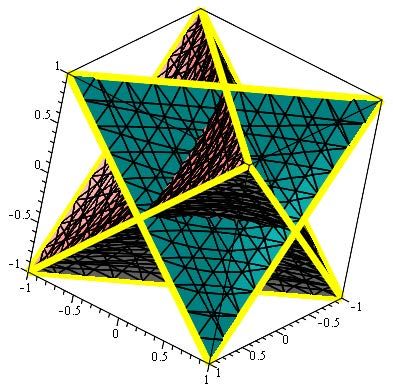
directed lengths of the four links. These eight bilinear factors can be viewed as the eight plane faces of a
regular stellated octahedron in the three-dimensional projective space implied by the four design parameter
directed lengths which may be interpreted as the four homogeneous coordinates of the space. The location of
a point in this parameter space relative to the octahedron predicts the mobility of the linkage. The numerical
values of the eight bilinear factors of the algebraic IO equation imply a complete classification scheme for
the relative mobility characteristics of the four links of these planar four-bar mechanisms.
This version of the paper is more comprehensive than the conference version, and intended for use as a
reference for the Project in MAAE 3004, Dynamics of Machinery. This version of the paper also includes
detailed notes on: exact kinematic synthesis of planar function generators using the algebraic IO equation;
the three species of double points of algebraic curves and their implications for the relative mobility of the
4R links; the projective extension of the Euclidean plane of the mechanism motion; interpretation of the
IO curves of mechanisms; angular velocity and acceleration level IO equation, and finally; determining 4R
mechanism coupler point curves. All other information, kinematics and kinetics, required to successfully
complete the tasks demanded by the project will be presented in the online course lectures and may also be
found in the MAAE 3004 required textbook: Theory of Machines and Mechanisms, 5th edition by Uicker,
Pennock, and Shigley.
Keywords: planar 4R linkages; kinematic synthesis; double points of planar algebraic equations; design
parameter space; link relative mobility classification; coupler point curves.
1 Thisterminology refers to a mechanical system comprising four rigid links connected to each other with four sequential revolute
joints (R-pairs) forming a closed 4R kinematic chain.
2021 CCToMM Mechanisms, Machines, and Mechatronics (M3 ) Symposium 11. INTRODUCTION
As James T. Kirk, Captain of the Starship Enterprise, may one day say many thousands of years from
now in a galaxy far, far away: “In the firmament of mechanical design the four-bar linkage burns as it’s
brightest star [1].” Indeed, four-bar linkages are ubiquitous. They can be identified in mechanical systems we
encounter every day: mechanical pencils; fold-out table-tops in class room chairs; bicycle lock mechanisms;
etc.. Ever since humans had the ability to formulate abstract thoughts, for countless thousands of years, four-
bar linkages, in their many forms, have been used to perform a large variety of tasks everywhere there have
been human beings [2]. However, only in the last 3000 years have the engineering sciences been applied,
in ever increasingly more sophisticated ways, to the synthesis and analysis of linkages for achieving desired
outputs for given inputs [3]. The science of mechanisms has evolved such that now nearly every article of
clothing you wear, the vehicles you are transported by, the household devices you use, even the streets you
walk on have all been touched by at least one, or two, if not many thousands, of four-bar linkages. These
mechanical systems can be designed to generate general displacements and motions in 3D space, on the
surface of a sphere, and in 2D space which we will call the Euclidean plane.
The term kinematic pair indicates a joint between two links, hence the use of the word pair. Joints
are mechanical constraints imposed on the links. Those involving surface contact are called lower pairs.
Those normally involving point, line, or curve contact are higher pairs. Lower pairs enjoy innate practical
advantages over higher pairs: applied loads are spread continuously over the contacting surfaces; they can,
in general, be more easily and accurately manufactured. There are six types of lower pair (see Figure 1)
classified in the following way [4].
1. R-Pair. The revolute R-pair is made up of two congruent mating surfaces of revolution. It has one
rotational degree-of-freedom (DOF) about its axis.
2. P-Pair. The prismatic P-pair comprises two congruent non-circular cylinders, or prisms. It has one
translational DOF. It’s axis is a line at infinity orthogonal to the direction of translation.
3. H-Pair. The helical H-pair, or screw, consists of two congruent helicoidal surfaces whose elements
are a convex screw and a concave nut. For an angle θ of relative rotation about the screw axis there
is a coupled translation of distance S in a direction parallel to the screw axis. The sense of translation
depends on the hand of the screw threads and on the sense of rotation. The distance S is the thread
pitch for a rotation of θ = 360◦ . When S = 0 it becomes an R-pair; when S = ∞ it becomes a P-pair.
The H-pair has one DOF specified as a translation or a rotation, coupled by the pitch S.
4. C-Pair. The cylindrical C-pair consists of mating convex and concave circular cylinders. They can
rotate relative to each other about their common axis, and translate relative to each other in a direction
parallel to the axis. Hence the C-pair has two DOF: one rotational, the other translational.
5. S-Pair. The spherical S-pair, also called ball-joints, consists of a solid sphere which exactly conforms
with a spherical shell. S-pairs permit three rotational DOF about intersecting orthogonal axes.
6. E-Pair. The planar E-pair (for the German word “ebene”, meaning “plane”) is a special S-pair com-
prising two concentric spheres of infinite radius. They permit two orthogonal translations and one
rotational DOF about an axis orthogonal to the plane of translation. They provide three DOF in total.
In one class of applications, the four-bar mechanism is driven by a human actuator. Examples of this
class are numerous, and sometimes taken for granted, e.g., when cutting a paper sheet with scissors, when
pedalling a bicycle, etc.. In the case of scissors, the two blades of this tool form a two-link open chain
coupled by an R-pair. When held by a user, this chain is coupled to a second, similar chain formed by the
2021 CCToMM Mechanisms, Machines, and Mechatronics (M3 ) Symposium 2Fig. 1. The six lower pairs: (a) revolute or pin; (b) prismatic; (c) helical; (d) cylindrical; (e) spherical; (f) planar.
Table 1. Summary of the lower pairs and their respective DOF.
Pair type Symbol DOF
Revolute R 1
Prismatic P 1
Helical H 1
Cylindrical C 2
Spherical S 3
Planar E 3
proximal phalanx of the thumb and the intermediate phalanx of the index finger, thereby forming a four-bar
linkage. Likewise, in the case of a bicycle, the frame and one of the two pedals form an open chain, which
couples with a second, similar chain, formed by the calf and the thigh of a human user, coupled by the R-pair
of the knee, thereby forming, again, a four-bar linkage.
In the context of planar mechanism kinematics, a dyad is a single rigid body link coupled to two other
rigid bodies with two kinematic pairs. The two other rigid bodies are a relatively non-moving ground link,
while the other is the coupler, which is connected to another dyad thereby forming a closed-loop four-bar
mechanism. The coupler is the link that joins, or couples, the two dyads. For planar displacements there are
only two types of lower pair that can be used to generate a motion in the plane: R- and P-pairs. This means
there are only four practical planar dyads
RR, PR, RP, and PP.
These 3-link serially connected open kinematic chains of rigid bodies are the building blocks of every planar
mechanism. They are designated according to the type of joints connecting the rigid links, and listed in series
starting with the joint connected to ground, each illustrated in Figure 2.
When a pair of dyads are coupled to each other, a four-bar linkage is obtained. However, the designation
2021 CCToMM Mechanisms, Machines, and Mechatronics (M3 ) Symposium 3y0
x0
Fig. 2. Types of dyads.
of the output dyad may change. For example, consider a planar four-bar linkage composed of an RR-dyad
on the left-hand side of the mechanism, and a PR-dyad on the right-hand side, where the input link is the
grounded link in the RR-dyad and the output link is the slider of the PR-dyad, see Figure 3.
coupler
Fig. 3. A four-bar linkage with RR-dyad on the left-hand side and PR-dyad on the right-hand side coupled via link l2
creates an RRRP mechanism.
Suppose revolute joint R1 is actuated by some form of torque supplied by an electric rotary motor trans-
ferred by a transmission, in turn driving the input link, l1 . The linkage is designated by listing the joints in
sequence from the ground fixed actuated joint, starting with the input link listing the joints in order. Thus,
the mechanism composed of a driving RR-dyad, and an output PR-dyad is called an RRRP linkage, where
the order of PR is switched to RP. If the output were an RP-dyad, the mechanism would be an RRPR linkage.
If the input were an RP-dyad while the output was an RR-dyad, the resulting mechanism would be an RPRR
linkage, with no noticeable alteration in the designation.
Because a four-bar mechanism possesses only a single DOF then only a single actuated input joint will
cause the three movable links to move. Two of the links are connected to the fixed base link of the mechanism
by either R- or P-pairs. Let us suppose that one of the joints connected to the fixed non-moving link is the
actuated joint. Now the other ground fixed link can be caused to move by a change in input of the actuated
joint, and the middle link couples the motion of the actuated input link to the non-actuated base fixed
2021 CCToMM Mechanisms, Machines, and Mechatronics (M3 ) Symposium 4moving link. Hence, the three relatively moving links in a four-bar mechanism are called the input, coupler, and output links respectively. If the mechanism links are joined by two R-pairs and two P-pairs then the coupler can move with general plane motion. That is, a coordinate system painted onto the coupler can both translate and rotate. If the linkage contains more than two P-pairs then the coupler coordinate system can only have curvilinear or linear displacements. For this reason, we will not discuss four-bar mechanisms containing more than two P-pairs. 2. INPUTS REQUIRED TO GENERATE DESIRED OUTPUTS We will presently briefly discuss the standard output motion generation problems associated with planar, spherical, and spatial four-bar mechanisms. While the input-output (IO) design problems listed next can be applied to mechanical systems of any kind, our focus will be mostly on planar 4R and RRRP mechanisms. The three most common design problems are termed function generation, motion generation, and path generation, which will now be discussed in that order. 2.1. Function Generation A function generating four-bar mechanism converts a change in input to a change in output correlated by a mathematical function. That is, the output is a desired function of the input. The classical problem of function generation was first formulated trigonometrically by Ferdinand Freudenstein in a seminal paper that has been recognized as the origin of modern kinematics [5]. For a four-bar 4R mechanism the design task becomes identifying the link lengths, which we abstractly define as the design parameters, in terms of the constant distances between sequential R-pair centres required to correlate the output link angle, over a prescribed range, as a desired mathematical function of the input angle. In an RRRP linkage the input is still an angle, but the output is a displacement along a line. Function generating mechanisms are found in sewing machines, washing machines, windshield wiper mechanisms, automotive suspensions, aircraft aileron mechanical systems, etc.. 2.2. Motion Generation The design task for motion generation, or rigid body guidance, involves identifying the design parameters of a four-bar mechanism that will guide the coupler through a desired motion. The coupler motion can be defined as the motion of any line on the coupler. Without loss in generality we may consider this as the motion of any coordinate system rigidly attached to the coupler. The motion of the coupler coordinate system consists of the translation of the origin of the coordinate system combined with its change in orienta- tion. Rigid body guidance is also known as the Burmester problem, since Ludwig Burmester published the very first recorded work in 1888 outlining a general solution [6]. Motion generating four-bar mechanisms are typically found in aircraft landing gear mechanisms, pick-and-place mechanical systems on automated assembly and packaging conveyors, camera pointing devices, etc.. 2.3. Path Generation Guiding a point along a desired path (curve) is, perhaps, the oldest four-bar linkage problem and was investigated by Archimedes more than two thousand years ago [3] and very likely by many others far earlier. In those times the mechanical devices that generated the desired curve were powered by humans, working animals, or water wheels. This design problem involves identifying the design parameters that will enable a point on the coupler to be guided along a desired curve over a desired range of motion. This point, known as the coupler point, is guided along the coupler point curve by the motion of the input link and the constraints imposed by the mechanism link lengths. The coupler point can be anywhere on the coupler, and is rarely on the line connecting the centres of the two R-pairs connecting the coupler to the input and output links. 2021 CCToMM Mechanisms, Machines, and Mechatronics (M3 ) Symposium 5
Coupler curves are quite complicated and subtle so we won’t dwell on them here. However, it is simple
to remember that coupler curves are of degree 6 (sextic) for 4R mechanisms, degree 4 (quartic) for RRRP
linkages, and degree 2 (quadratic) for PRRP linkages.
   The steam age spawned the Industrial Revolution in the 1700s. Coal was needed to boil water to generate
the steam that powered the revolution. The need to pump water out of coal mines in England led James Watt
to devise a straight line linkage that could transfer the oscillating input of a steam power driven piston to a
rotating link connected to the piston by a coupler. The concept of the mechanism was patented in 1784 [7].
The coupler was also connected, via an R-pair, to a pumping piston. Thus the power generated by the steam
driven piston was transferred to the pumping mechanism which, by design, only needed to do work along
the straight line portion of the coupler curve. The Watt linkage, illustrated in Figure 4a, is designed to move
point C, located at the midpoint of the coupler, approximately along a straight line over a portion of the
curve on which it is constrained to move. This linkage it is still widely used in a large variety of automotive
and locomotive suspension systems.

                          (a) Watt straight line linkage.                                (b) Watt coupler curve.

             Fig. 4. Watt straight-line linkage and coupler point curve where a1 = a3 = 10 and a2 = 2.

  The link length conditions for an arbitrary Watt mechanism are as follows. The input and output links
have the same length, a1 = a3 . The coupler point C is located at a2 /2 along the longitudinal centre line
of the coupler. The distance between the centres of the two ground-fixed R-pairs can be expressed by
the coordinates
     q          in the x0 − y0 coordinate system as (2a1 , a2 ), and the distance between the two centres is
a4 = (2a1 )2 + a22 . The longest link is always a4 . The coupler point curve for the Watt linkage illustrated
in Figure 4a is plotted in Figure 4b.
   The mobility constraints on the input and output links are determined by the numerical values of the linear
coefficient factors A1 , C1 , and D1 of Equation (1) are [1]:
                                            A1 = a1 − a2 − a3 + a4 ,
                                            C1 = a1 − a2 + a3 − a4 ,
                                            D1 = a1 + a2 − a3 − a4 .
Because a1 = a3 and a4 always represents the longest link length in a Watt mechanism then A1 is always a
positive non-zero number while D1 is always a negative non-zero number. Moreover, C1 is always a negative

2021 CCToMM Mechanisms, Machines, and Mechatronics (M3 ) Symposium                                                 6
non-zero number as well since 2a1 < a2 + a4 . Therefore, a Watt straight line mechanism is always a non-
Grashof 0-rocker-π-rocker, according to the planar 4R input-output link mobility classification found in [1],
and reproduced here as Table 2.
# A1 C1 D1 Input a1 Output a3 # A1 C1 D1 Input a1 Output a3
1 + + + 0-rocker 0-rocker 15 0 0 - crank π-rocker
2 + + 0 0-rocker 0-rocker 16 0 - + π-rocker crank
3 + + - rocker rocker 17 0 - 0 crank crank
4 + 0 + 0-rocker crank 18 0 - - crank π-rocker
5 + 0 0 0-rocker crank 19 - + + crank crank
6 + 0 - 0-rocker π-rocker 20 - + 0 crank crank
7 + - + rocker crank 21 - + - π-rocker π-rocker
8 + - 0 0-rocker crank 22 - 0 + crank crank
9 + - - 0-rocker π-rocker 23 - 0 0 crank crank
10 0 + + crank crank 24 - 0 - crank π-rocker
11 0 + 0 crank crank 25 - - + π-rocker 0-rocker
12 0 + - π-rocker π-rocker 26 - - 0 crank 0-rocker
13 0 0 + crank crank 27 - - - crank rocker
14 0 0 0 crank crank
Table 2. Classification of all possible planar 4R linkages. Shaded cells satisfy the Grashof condition.
Path generating linkages are now very common in automated manufacturing and assembly operations.
Consider an automobile assembly station where windshields are attached to the vehicle body. A uniform
bead of adhesive must be applied to the windshield just before a robotic arm picks it up and places it in the
precise location on the gasket in the windshield opening on the body. This adhesive is typically applied by
a four-bar linkage where the point on the coupler that follows the required adhesive bead path is generated
by the input link rotating with constant angular velocity. However, in this case the adhesive bead must be
uniform. This means that the coupler point, the nozzle of the adhesive applicator, must also have a constant
velocity as it moves along the coupler point curve. Therefore the designer must simultaneously address the
position level and velocity level kinematics.
3. PLANAR 4R LINKAGES
The planar 4R four-bar linkage, colloquially known as a crank-rocker, drag-link (also known as a double-
crank), or double-rocker depending on the link lengths, has been a workhorse in the realm of mechanical and
aerospace engineering for centuries, if not millennia [3]. While trigonometric analytical methods to study
the relationship between the motions of the input and output links, based on the distances between the R-pair
centres have existed for at least 150 years [8], purely algebraic methods have not. This means that the theory
of algebraic differential geometry [9, 10] cannot be used to identify the structure of the relationship between
the input and output parameters. Still, trigonometric methods are highly accessible and largely intuitive. The
trigonometric input-output (IO) equations for planar 4R linkages that have become the backbone of analysis
and synthesis were first introduced by Ferdinand Freudenstein in the 1950s [5, 11]. The same trigonometric
approach has been used for planar RRRP linkages as well as for those containing as many as two P-pairs [2].
The algebraic IO equation for a planar 4R linkage is an algebraic polynomial that relates the tangent half-
angle parameter of the input joint angle to the tangent half-angle parameter of the output joint angle in terms
2021 CCToMM Mechanisms, Machines, and Mechatronics (M3 ) Symposium 7of the link lengths [12, 13]. A polynomial is algebraic if the coefficients are rational numbers2 . This IO
equation can be derived algorithmically [14] without explicit reference to trigonometry using the Denavit-
Hartenberg (DH) parametrisation of the linkage kinematic geometry [15], Study’s kinematic mapping [16],
and Gröbner bases [17, 18]. Algebraic IO equations for any closed RRRP and PRRP kinematic chain can
be similarly derived from the kinematic geometry but, as it turns out, this is unnecessary. Recent work by
Rotzoll et al. [14, 19] has yielded the remarkable result that the algebraic IO equations for planar four-bar
linkages that contain one, two, three, or even four P-pairs are embedded in the general planar 4R algebraic
IO equation. That is, one need only collect the planar 4R algebraic IO equation in terms of the variable
input and output parameters. Regardless, these algebraic IO equations can be derived from the kinematic
geometry. The interested reader is referred to [20] for details.
Fig. 5. Planar 4R closed kinematic chain.
Consider the planar 4R closed kinematic chain illustrated in Figure 5. The basis vector directions of the
non-moving coordinate reference system are x0 -y0 . The coordinate system origin is located at the rotation
centre of the input link ground-fixed R-pair, while the x0 -axis points towards the rotation centre of that of the
output link. The algebraic IO equation of an arbitrary planar 4R linkage illustrated in Figure 5 is represented
as
Av21 v24 + Bv21 +Cv24 − 8a1 a3 v1 v4 + D = 0, (1)
where
A = (a1 − a2 − a3 + a4 )(a1 + a2 − a3 + a4 ) = A1 A2 ;
B = (a1 − a2 + a3 + a4 )(a1 + a2 + a3 + a4 ) = B1 B2 ;
C = (a1 − a2 + a3 − a4 )(a1 + a2 + a3 − a4 ) = C1C2 ;
D = (a1 + a2 − a3 − a4 )(a1 − a2 − a3 − a4 ) = D1 D2 ;
θ1 θ4
v1 = tan ; v4 = tan .
2 2
The joint angle parameters v1 and v4 represent the tangent half-angles of linkage input and output angles, θ1
and θ4 . The eight bilinear factors of the coefficients A, B, C, and D in Equation (1) depend on the numerical
values of the four ai link lengths. In this formulation the input link, a1 , is always positive but the remaining
three ai directed distances are the unique eight permutations of positive and negative signs in each factor.
Hence, the eight bilinear factors represent eight distinct planes. Note that these permutations in sign only
2A rational number can be expressed exactly as the ratio√of two integers. The number 3.333 · · · is rational because it can be
expressed exactly by the ratio 1/3, whereas the number 2 is irrational because it cannot be expressed exactly by such a ratio.
2021 CCToMM Mechanisms, Machines, and Mechatronics (M3 ) Symposium 8applies to the arithmetic operations of addition and subtraction, they do not represent the sign of the numeric
value of the directed length. Treating the four ai as homogeneous coordinates with a4 as the homogenising
coordinate one can uniformly scale the numerical values of the four ai by dividing by a4 , which is always an
arbitrary nonzero number for any real 4R linkage, without affecting the functional relationship v4 = f (v1 ).
Treating the ai as mutually orthogonal basis directions in the hyperplane a4 = 1, the eight planes intersect in
the only uniform polyhedral compound [21], called the stellated octahedron, which has order 48 octahedral
symmetry: a regular double tetrahedron that intersects itself in a regular octahedron [22]. The location of
a point in this space completely determines the relative mobility of all four links and hence it is termed the
design parameter space of planar 4R linkages.
There has always existed an almost innate understanding that as the radius of a sphere tends towards
infinity it can be considered as the plane at infinity. Projective geometry has, of course, shown that this is
indeed the case mathematically [23]. The axes of a spherical 4R linkage intersect at the centre of the sphere,
see the spherical 4R illustrated in Figure 6b, while those of a planar 4R are mutually parallel but intersect in
a unique point on the line at infinity in the projective extension of the Euclidean plane of the 4R mechanism.
Therefore, there arose the notion in the 1800’s that planar 4R mechanisms are special cases of spherical 4R
linkages on the surface of a sphere of infinite radius. This notion was proved to be true in [24] and more
recently in [14] where the proof is relatively straightforward using the algebraic form of the IO equation.
a3, a3
a1 a2, a2 a1, a1
(a) (a) Twelve lines common to the spherical and pla-
nar 4R design parameter spaces. (b) A spherical 4R mechanism.
Fig. 6. Design parameter space intersections and a planar RRRP linkage.
The design parameters of a spherical 4R are four nonzero arc length angle parameters, which are the
tangent half-angle parameters, αi , of the arc length angles, τi , such that αi = tan (τi /2). The algebraic IO
equation of a spherical 4R contains eight bicubic factors in the αi . These eight cubic factors are singular
cubic surfaces [21] in the sense that they all contain only 12 and not the maximum number of 27 lines [25].
Each cubic surface contains three real finite lines which intersect in an equilateral triangle and different pairs
of the eight cubic surfaces have a different line in common. Treating the four αi as mutually orthogonal
basis directions and projecting into the hyperplane α4 = 1 reveals the design parameter space of spherical
4R linkages. Each distinct point in this space is a unique spherical 4R and the mobility of the input and
output links is completely determined by its location in this space. It turns out that the eight cubic surfaces
in the spherical 4R design parameter space intersect the planar 4R design parameter space in the 12 edges of
the double tetrahedra, see Figure 6a. The vertices of the tetrahedra are the vertices of the equilateral triangles
on each cubic surface while the edges are the lines themselves.
2021 CCToMM Mechanisms, Machines, and Mechatronics (M3 ) Symposium 93.1. Planar 4R Algebraic IO Equations
a2
'2 3
a1
y0 2 a3
4
1
x0
a4
Fig. 7. Planar 4R Joint Angles.
Consider the planar 4R linkage illustrated in Figure 7. The standard variables are the a1 and a3 joint
angles θ1 and θ4 . But we can choose any pair of links to act as “input” and as “output” meaning that there
are five additional IO pairings, in addition to Equation (1), reprinted here as Equation (2) for convenience.
The six possible algebraic IO equations are [26]:
Av21 v24 + Bv21 +Cv24 − 8a1 a3 v1 v4 + D = 0, (2)
where
A = A1 A2 = (a1 − a2 − a3 + a4 )(a1 + a2 − a3 + a4 ),
B = B1 B2 = (a1 − a2 + a3 + a4 )(a1 + a2 + a3 + a4 ),
C = C1C2 = (a1 − a2 + a3 − a4 )(a1 + a2 + a3 − a4 ),
D = D1 D2 = (a1 + a2 − a3 − a4 )(a1 − a2 − a3 − a4 ),
v1 = tan θ21 ,
v4 = tan θ24 ;
the five other algebraic IO equations are
A1 B1 v21 v22 +A2 B2 v21 +C1 D2 v22 +8a2 a4 v1 v2 +C2 D1 = 0; (3)
A2 B1 v21 v23 + A1 B2 v21 +C1 D1 v23 +C2 D2 = 0; (4)
B1C1 v22 v23 +A1 D2 v22 +A2 D1 v23 −8a1 a3 v2 v3 +B2C2 = 0; (5)
A1C1 v22 v24 + B1 D2 v22 + A2C2 v24 + B2 D1 = 0; (6)
A2C1 v23 v24 +B1 D1 v23 +A1C2 v24 +8a2 a4 v3 v4+B2 D2 =0. (7)
3.1.1. vi -v j Input-output Curves
Consider a planar 4R linkage where a1 = 2, a2 = 6, a3 = 8, a4 = 5 in generic units of length. Substituting
these link lengths into Equation (2) yields:
−35v21 v24 + 189v21 − 128v1 v4 − 11v24 + 85 = 0.
2021 CCToMM Mechanisms, Machines, and Mechatronics (M3 ) Symposium 10Making an implicit plot in Maple reveals the v1-v4 curve over a specified range of bounding values for the
two numbers defined by tan (θi /2) illustrates the curves in each assembly mode. The implicit plot command
works by evaluating a number of points on the curve that you can specify, then solving the equation for v4
for each incremental value of v1 . However, the v1 -v4 IO curves illustrated in Figure 8 were created with
GeoGebra to show both the coupler point and IO curves. Substituting the link lengths into the remaining
five vi -v j IO equations (3) through (7) reveal the functional correlation between the specified pair of joint
angle parameters in Figures 9 through 11.
(a) v1 -v4 IO and coupler curves, upper assembly (b) v1 -v4 IO and coupler curves, both assembly
mode. modes.
Fig. 8. Planar 4R v1 -v4 IO and coupler curves for a1 = 2, a2 = 6, a3 = 8, and a4 = 5.
Fig. 9. Planar 4R v1 -v2 and v1 -v3 IO curves for a1 = 2, a2 = 6, a3 = 8, and a4 = 5.
Examining the figures, we can immediately deduce the relative angular displacement ranges between the
associated joint angle parameter pairs. Figure 8 indicates that Link a1 is a crank and a3 is a rocker, both
relative to a4 . Figures 9 indicate that a1 is a crank relative to a4 while a2 is also a crank relative to a1 for
the v1 -v2 IO curve and a1 is a crank relative to a4 while a3 is a rocker relative to a1 for the v1 -v3 IO curve.
2021 CCToMM Mechanisms, Machines, and Mechatronics (M3 ) Symposium 11Fig. 10. Planar 4R v2 -v3 and v2 -v4 IO curves for a1 = 2, a2 = 6, a3 = 8, and a4 = 5.
Fig. 11. Planar 4R v3 -v4 IO curve for a1 = 2, a2 = 6, a3 = 8, and a4 = 5.
Figures 10 indicate that a2 is a crank relative to a1 while a3 is rocker relative to a2 for the v2 -v3 IO curve
and a2 is a crank relative to a1 while a4 is a rocker relative to a3 for the v2 -v4 IO curve. Lastly, Figure 11
reveals that a3 is a rocker relative to a4 while a4 is rocker relative to a3 for the v3 -v4 IO curve.
3.2. Mobility Classification
The double points at infinity belonging to each of the four distinct vi coordinate axes together with the type
of points at vi = 0 completely define the mobility limits, if they exist, between each vi -v j angle parameter
pair. Physically speaking, these two points correspond to the two extreme orientations implied by the vi
where the two links can align. Hence, the examination of these two points is sufficient to determine whether
a particular joint enables a crank, a rocker, a π-rocker, or a 0-rocker link motion [1]. This may help clarify
some of the terms found in Table 2.
2021 CCToMM Mechanisms, Machines, and Mechatronics (M3 ) Symposium 123.2.1. Double Points
Before examining the classification, double points require some discussion. Each point of each distinct
branch of an algebraic curve possesses at least one distinct tangent. What happens if the curve does not
possess distinct branches or if the curve self-intersects? If a curve intersects itself then there must be more
than one tangent to the curve at the self-intersection location. How can a point of the curve that possesses
two, or more, tangents be classified? In the study of the kinematic geometry of mechanisms [27], and
of algebraic differential geometry in general [9, 10], these special locations have important meanings for
linkage velocities, accelerations, and jerks. These locations are usually called multiple points because there
are multiple tangents at that point. They are also called singular points because the point is uniquely defined
at that location, and hence singular. However, work with planar four-bar linkages requires only knowledge
of double points, locations where a curve intersects itself a single time. A comprehensive account of multiple
points can be found in [28] for the interested reader.
There are three species of double point that arise when the tangents to the curve at the double point are
either a pair of distinct real lines, a pair of complex conjugate lines, or a pair of real but coincident lines.
Methods to analytically identify the presence of double points of an algebraic curve and to determine the
class of the double point are discussed next. The type of double point can be used to classify the mobility
capability of input link.
To illustrate the different nature of the three types of double point consider the following cubic equation
y2 = (x − a)(x − b)(x − c) (8)
where the constant coefficients have rational positive magnitudes such that a < b < c. This curve, illustrated
in Figure 12a, is symmetric with respect to the x-axis since every value of x gives equal and opposite values
of y. The curve intersects the x-axis at the three points x = a, x = b, and x = c. When x < a the value of y2 is
negative, and y is imaginary. When a < x < b then y2 is positive, and there are two real, equal and opposite
values for y. For values of b < x < c the value for y2 is again negative, and finally positive again for all
values x > c. The curve therefore consists of a closed oval between a and b and an open branch beginning at
c and extending infinitely in two directions beyond it. The curve illustrated in Figure 12a has a = 2, b = 4,
and c = 5. These values will now be manipulated to yield examples of the three types of double point.
b=c
a b c a
(a) Cubic with two real branches and no double points. (b) A regular double point, or crunode.
Fig. 12. Species of double points: regular.
Expanding Equation (8) and collecting the terms in descending powers of x and y leads to a polynomial
equation, f (x, y) = 0:
f (x, y) := x3 − (a + b + c)x2 + (ab + ac + bc)x − y2 − abc = 0. (9)
2021 CCToMM Mechanisms, Machines, and Mechatronics (M3 ) Symposium 13Let b vary in magnitude between the range a ≤ b ≤ c. As b increases in value the oval circuit increases
in size maintaining it’s location at a but growing towards c until b = c and the curve crosses itself. In this
example a = 2 and b = c = 5. Inspecting the curve illustrated in Figure 12b we see that at the double point,
or node, the two branches of the curve meet, and each branch has it’s own real, distinct tangent. Such a point
is called a regular double point, or a crunode. There is only one common zero of Equation (9) and it’s partial
derivatives with respect to x and y: (x, y) = (5, 0). The discriminant of Equation (9) given by Equation (14)
is
∆ = 12x − 48. (10)
Evaluating Equation (10) at the double point (x, y) = (5, 0) leads to
∆ = 12 > 0,
which is a positive non-zero number, as it must be, since the multiple point is a regular double point, or
crunode.
As b moves in the opposite direction towards a, the original oval circuit in Figure 12a now shrinks in size
until b = a, giving for a = b = 2 and c = 5
x3 − 9x2 + 24x − y2 − 20 = 0. (11)
as illustrated in Figure 13a. The cubic now possesses an isolated double point at x = a = b = 2. Isolated
double points, also known as acnodes or hermit points, satisfy the equation of the cubic but do not appear to
lie on the curve. The tangents to the curve at an isolated double point are a pair of complex conjugate lines.
No real line through the isolated double point intersects the curve in more than two real points, confirming
the necessary condition that a general real line cuts a cubic in three points. The reader should confirm that
the common solution to Equation (11) and it’s partial derivatives with respect to x and y is (x, y) = (2, 0),
and that the discriminant of Equation (11) evaluated at the double point is
∆ = −12 < 0.
The result is a number less than zero, as it must be, since this is an isolated double point, or acnode.
a=b c a=b=c
(a) An isolated double point, or acnode, or hermit point. (b) A stationary double point, or spinode , or cusp.
Fig. 13. Species of double points: isolated and stationary.
The third species of double point occurs if the equation of the tangent to the curve at a point becomes a
perfect square. In this case the tangents at the self-intersection point, called a stationary double point are
2021 CCToMM Mechanisms, Machines, and Mechatronics (M3 ) Symposium 14two real, but coincident lines. In the case of the cubic in Equation (8), if we allow both coefficients b and
c to approach a then the two distinct branches of the curve merge into a single branch when a = b = c and
Equation (8) becomes
y2 = (x − a)3 . (12)
When expanded and collected in terms of descending powers of x and y then Equation (12) can be expressed
as the polynomial equation for a = b = c = 2
x3 − 6x2 + 12x − y2 − 8 = 0. (13)
This situation is illustrated in Figure 13b. The stationary double point where x = a = b = c is also called a
cusp or a spinode. They are called stationary double points because if the curve is generated by the motion
of a point then at a cusp the motion of the point in one direction comes to a stop and changes direction
making the velocity of the point instantaneously zero at the stationary double point coordinates. The tangent
at the cusp meets the curve in three coincident points at (a, 0) in Figure 13b. The reader should confirm that
the common solution to Equation (13) and it’s partial derivatives with respect to x and y is (x, y) = (2, 0),
and that the discriminant of Equation (13) evaluated at the double point is
∆ = 0.
The differential geometry implied by the discriminant demands that it’s value, evaluated at the stationary
double point (x, y) = (2, 0), is identically equal to zero.
3.2.2. Homogeneous Coordinates
Let O be the origin of the Cartesian coordinate system, shown in Fig-
ure 14. Let S be a distinct point in the plane. The ray passing through
O and S is described by the coordinate pair (x, y). Another distinct
point Q ̸= O, on ray OS is described by the pair (µx, µy), where
µ ∈ R (ie., a real number). As µ → ±∞ the seemingly meaningless
pair (∞, ∞) is obtained [29].
To remedy this representational problem, the point pairs may be
represented by two ratios, given by ordered triples (x0 , x1 , x2 ). If x0 ̸=
0, then the point S can be uniquely described as:
x1 x2
x= , y= . Fig. 14. Cartesian coordinates in E2 .
x0 x0
Then any triple of the form (λ x0 , λ x1 , λ x2 ), for λ ̸= 0, describes exactly the same point S. In other words,
two real points are equal if the triples representing them are proportional. This is because
λ x1 x1 λ x2
= = x, and = y.
λ x0 x0 λ x0
The corresponding coordinates (x0 : x1 : x2 ) are called homogeneous coordinates, but are really three ratios.
This is indicated with the symbol : in the set of homogeneous coordinates. When x0 = 1 the Cartesian
coordinate pair (x, y) is recovered.
2021 CCToMM Mechanisms, Machines, and Mechatronics (M3 ) Symposium 153.2.3. Mobility Classification Conditions
One possibility to determine the type of double point, i.e., whether it is a crunode, acnode, or cusp, is to
evaluate whether the double point has a pair of real, or complex conjugate tangents. If the double point has
two real distinct tangents, it is a crunode; if it has two real coincident tangents, it is a cusp; and if the tangents
are both complex conjugates, the double point is an acnode [9, 30]. Thus, after homogenising each vi -v j
angle pair IO equation using the homogenising coordinate v0 , leading to IOh , the following discriminant
yields information on the double point at infinity on the v j axis:
2 > 0 ⇒ crunode;
∂ 2 IOh ∂ 2 IOh ∂ 2 IOh
∆= − = 0 ⇒ cusp; (14)
∂ vi ∂ v0 ∂ v2i ∂ v20 < 0 ⇒ acnode.
To obtain, for example, the homogeneous v1 -v4 IO equation of an arbitrary planar 4R linkage we must
redefine the (v1 , v4 ) coordinates as three homogeneous ratios. The discriminant of the point at infinity
(v0 : v1 : v4 ) = (0 : 1 : 0) on the v1 -axis is obtained by setting i = 4 in the discriminant equation, i.e. ∂ v4 ,
while the discriminant of the other point at infinity (v0 : v1 : v4 ) = (0 : 0 : 1) on the v4 -axis is obtained by
setting i = 1 in the discriminant equation, i.e. ∂ v1 .
Proceeding with the double point analysis of all six vi -v j equations at infinity on both axes results in 12
discriminants. However, as the vi -v j equations are all dependent on each other, from the 12 discriminants
we are left with only four distinct ones describing the nature of the double points at infinity of each vi for
i ∈ {1...4}. The complete derivation can be found in [26], but in that paper different coordinate systems are
used meaning that the coefficients have different definition from those defined in this tutorial in Equation (2).
Using the coordinate system definitions observed in Figure 5 it can be shown that the conditions on the
angular mobility of one of the four links, relative to the link with respect to which the angle is measured, are
listed in Tables 3-6, where the eight bilinear factors A1 -D2 are defined in Equation (2). This approach to the
angular mobility classification of the individual links provides an arguably more general set of conditions
than those found in Table 2.
Table 3. Mobility limits of a1 . Table 4. Mobility of a2 .
C1C2 D1 D2 A1 A2 B1 B2 mobility of a1 A1 B1C1 D2 A2 B2C2 D1 mobility of a2
≤0 ≤0 crank ≤0 ≤0 crank
≤0 >0 π-rocker ≤0 >0 π-rocker
>0 ≤0 0-rocker >0 ≤0 0-rocker
>0 >0 rocker >0 >0 rocker
Table 5. Mobility of a3 . Table 6. Mobility of a4 .
A2 B1C1 D1 A1 B2C2 D2 mobility of a3 A1 A2C1C2 B1 B2 D1 D2 mobility of a4
≤0 ≤0 crank ≤0 ≤0 crank
≤0 >0 π-rocker ≤0 >0 π-rocker
>0 ≤0 0-rocker >0 ≤0 0-rocker
>0 >0 rocker >0 >0 rocker
3.2.4. Computing Critical Input Angles to Determine Output Angle Extreme Values
If the mobility classification reveals that angular displacement limits exist for a link in a planar 4R mech-
anism, how can the numerical values of the limits be computed? This task is efficiently accomplished using
differential calculus. Consider the mobility limits for the 4R linkage IO curve illustrated in Figure 8b where
2021 CCToMM Mechanisms, Machines, and Mechatronics (M3 ) Symposium 16a1 = 2, a2 = 6, a3 = 8, and a4 = 5. The v1 -v4 algebraic IO equation for these link lengths is reproduced here
for convenience:
−35v21 v24 + 189v21 − 128v1 v4 − 11v24 + 85 = 0. (15)
To determine the angle parameter limits between which the output link a3 rocks in each assembly mode
requires the critical values v1crit at which the limiting values of v4 occur. First solve Equation (15) for v4 :
q
−64v1 ± 615v41 + 9150v21 + 935
v4 = . (16)
35v21 + 11
Each solution in Equation (16) represents the value of v4 for a specified value of v1 in each assembly mode.
To determine the two values of v1crit in each assembly mode, the derivative of Equation (16) must be taken
with respect to v1 . Solve the resulting derivatives for v1crit that satisfy
dv4
= 0. (17)
dv1
In this example, we find for one assembly mode that
√ √
231 197
v1crit = and, − , (18)
21 21
while for the other assembly mode we find
√ √
231 197
v1crit = − and, . (19)
21 21
Substituting each value for v1crit into Equation (16) reveals the corresponding extreme values for v4 , listed
in Table 7. The angle equivalents for θ1crit and θ4min/max are listed in Table 8. Figures 15 and 16 illustrate the
linkage in its extreme configurations in each assembly mode.
Table 7. v4min/max .
v4 Assembly Mode 1 Assembly Mode 2
v4min 1.381698560 -1.381698560
v4max 4.675162334 -4.675162334
Table 8. θ1crit and θ4min/max .
Assembly Mode 1 Assembly Mode 2 Assembly Mode 1 Assembly Mode 2
71.79004310◦ 54.90036778◦ 108.2099569◦ -155.85315208◦
θ1crit θ4min/max
-54.90036778◦ -71.79004310◦ 155.85315208◦ -108.2099569◦
2021 CCToMM Mechanisms, Machines, and Mechatronics (M3 ) Symposium 17(a) Configuration for θ4min . (b) Configuration for θ4max
Fig. 15. Assembly Mode 1 θ1crit and θ4min/max .
(a) Configuration for θ4min . (b) Configuration for θ4max
Fig. 16. Assembly Mode 2 θ1crit and θ4min/max .
3.3. Planar 4R Algebraic Angular Velocity IO Equations
The equation relating the time rates of change of the joint angle parameters v1 and v4 can be determined
as the first time derivative of Equation (2):
(Av24 +B)v1 −4a1 a3 v4 v̇1 + (Av21 +C)v4 −4a1 a3 v1 v̇4 .
(20)
Because Equation (20) equates to zero, the velocity parameter ratio can be expressed as
v̇4 (Av24 + B)v1 − 4a1 a3 v4
= − , (21)
v̇1 (Av21 +C)v4 − 4a1 a3 v1
2021 CCToMM Mechanisms, Machines, and Mechatronics (M3 ) Symposium 18which can also be directly obtained as the implicit derivatives of Equation (2) with respect to v1 and v4 . It is
important to note that for the ith link, v̇i ̸= θ̇i since vi = tan (θi /2). But it is a simple matter to show that
θ̇i (1 + v2i )
v̇i = , (22)
2
and that
2v̇i
θ̇i = . (23)
(1 + v2i )
Hence, the reciprocal of the mechanical advantage is
θ̇4 ((Av24 + B)v1 − 4a1 a3 v4 )(1 + v21 )
= − . (24)
θ̇1 ((Av21 +C)v4 − 4a1 a3 v1 )(1 + v24 )
The remaining angular velocity equations are expressed as the following ratios
θ̇2 ((A1 B1 v22 + A2 B2 )v1 + 4a2 a4 v2 )(1 + v21 )
= − , (25)
θ̇1 ((A1 B1 v21 +C1 D2 )v2 + 4a2 a4 v1 )(1 + v22 )
θ̇3 ((A2 B1 v23 + A1 B2 )v1 )(1 + v21 )
= − , (26)
θ̇1 ((A2 B1 v21 +C1 D1 )v3 )(1 + v23 )
θ̇3 ((B1C1 v23 + A1 D2 )v2 − 4a2 a4 v3 )(1 + v22 )
= − , (27)
θ̇2 ((B1C1 v22 + A2 D1 )v3 − 4a2 a4 v2 )(1 + v23 )
θ̇4 ((A1C1 v24 + B1 D2 )v2 )(1 + v22 )
= − , (28)
θ̇2 ((A1C1 v22 + A2C2 )v4 )(1 + v24 )
θ̇4 ((A2C1 v24 + B1 D1 )v3 − 4a2 a4 v4 )(1 + v23 )
= − , (29)
θ̇3 ((A2C1 v23 + A1C2 )v4 − 4a2 a4 v3 )(1 + v24 )
P24
P23
a2
a3
a1 P12
y0
x0 a4
P13 P14 P34
Fig. 17. The six instantaneous centres of velocity.
2021 CCToMM Mechanisms, Machines, and Mechatronics (M3 ) Symposium 193.4. Generalisation of Freudenstein’s Theorem 1
Consider the planar 4R linkage illustrated in Figure 17. It is well known that as the 4R linkage moves
it has four primary instantaneous centres of velocity (ICV), one at the centre of each R-pair. Two of the
primary ICVs, P12 and P23 , move on centrodes defined by the link lengths, while P14 and P34 are stationary.
The two secondary ICVs are P13 and P24 , which also move on centrodes. By virtue of the Aronhold-Kennedy
theorem, P13 , P14 , and P34 remain collinear as the motion evolves over time meaning that the centrode for
P13 is the line joining the two ground-fixed R-pairs, the x0 -axis, and is located at the point of intersection of
the x0 -axis and the extension of the centreline of the coupler, a2 . Freudenstein’s Theorem 1 [31, 32] states
that the value of the ratio of the output angular velocity and the input angular velocity, θ̇4 and θ̇1 , can be
expressed by the ratio of the values of the relative directed distances between the three ICVs located on the
x0 -axis in the following way:
θ̇4 dP13 P14
= , (30)
θ̇1 dP13 P14 + dP14 P34
where the directed distances dP14 P34 and dP13 P14 can be positive or negative depending on their relative direc-
tions.
It is a straightforward computation to express the value of the location of P13 as the point of intersection
of the longitudinal centreline of the coupler and the line containing the x0 -axis in terms of the link directed
lengths and the joint angle parameters v1 and v4 as
!
a1 (a3 v21 v4 −a3 v1 v24 +a4 v1 v24 +a3 v1 −a3 v4 +a4 v1)
a1 v1 v24 − a3 v21 v4 + a1 v1 − a3 v4
!. (31)
a1 (a3 v21 v4 −a3 v1 v24 +a4 v1 v24 +a3 v1 −a3 v4 +a4 v1)
+a4
a1 v1 v24 − a3 v21 v4 + a1 v1 − a3 v4
Selecting a configuration of a viable planar 4R and substituting the appropriate values it is a simple matter
to show that the values of Equations (24), (30), and (31) are equivalent. For example, substituting the ai
values of a1 = 7, a2 = 13, a3 = 8, a4 = 16, v1 = tan (60/2) and v4 = tan (87.4498/2) into the three equations
leads to the identical result
v̇4 (1 + v21 )
= 0.6974. (32)
v̇1 (1 + v24 )
However, Freudenstein’s first theorem also applies to the ICVs on each of the three other Aronhold-Kennedy
lines of three collinear ICVs with respect to a number line coincident with the line of three ICVs having its
Table 9. Configuration parameters for a closed 4R chain.
Parameter Dimension Parameter Dimension
a1 5 dP13 P14 -32.4571
a2 6 dP13 P12 -29.1205
a3 8 dP24 P12 6.6954
a4 2 dP24 P23 11.4161
θ1 45◦ θ3 207.5141◦
θ2 308.0304◦ θ4 20.5445◦
2021 CCToMM Mechanisms, Machines, and Mechatronics (M3 ) Symposium 20origin on the central ICV. It seems that, to the best of the authors collective knowledge, this fact has never
been discussed in the literature. The six ICVs are known as velocity poles and the curves they move along
are described as polodes, see [2, 4, 33, 34] for example. However, it seems that the following three velocity
ratios expressed as ratios of the absolute values of the relative locations of the three ICVs on the three other
Aronhold-Kennedy lines, see Figure 17, have never been stated explicitly as:
θ̇1 dP24 P12
= ; (33)
θ̇2 dP24 P12 + dP12 P14
θ̇3 dP13 P12
= ; (34)
θ̇2 dP13 P12 + dP12 P23
θ̇4 dP24 P23
= . (35)
θ̇3 dP24 P23 + dP23 P34
Additionally, Equations (25) and (28) are angular velocity ratios in terms of distance and configuration.
These results yield a measure of all six angular velocity ratios with the six additional Equations (24)-(29).
3.5. Example: Velocity Ratio
In this section we shall illustrate the validity of our generalised Freudenstein theorem ratios of relative
distances between ICVs on the four Aronhold-Kennedy lines and explicitly computed angular velocity ra-
tios. For this example the linkage and configuration illustrated in Figure 17 is used with the lengths (generic
units) and angles (degrees) listed in Table 9.
Using these parameters, the four Aronhold-Kennedy lines, and the extended Freudenstein theorem yields:
dP13 P14 θ̇4
= 1.0657 = ;
dP13 P14 + dP14 P34
θ̇1
dP24 P12 θ̇1
= −3.9492 = ;
dP24 P12 + dP14 P12
θ̇2
(36)
dP13 P12 θ̇3
= −1.2595 = ;
dP13 P12 + dP12 P23 θ̇2
dP24 P23 θ̇4
= 3.3419 = .
dP24 P23 + dP23 P34 θ̇3
The negative or positive sign multiplying the ratio indicates whether or not the two angular velocities have
the same sense. Compared to the angular velocities obtained with the six angular velocity ratios computed
with suitable variants of Equation (24), we obtain four identical ratios in addition to two, which are not
possible to compute directly as ratios of ICVs:
θ̇4 θ̇3
= 1.0657; = −1.2595;
θ̇1 θ̇2
θ̇1 θ̇4
= −3.9492; = −4.2085; (37)
θ̇2 θ̇2
θ̇3 θ̇4
= 0.3189; = 3.3419.
θ̇1 θ̇3
2021 CCToMM Mechanisms, Machines, and Mechatronics (M3 ) Symposium 21P24
xis
n A P23
tio a2
n ea
lli
Co
a3
a1 P12 .
y0 . 4
1
x0 a4
P13 P14 P34
Fig. 18. The collineation axis.
3.6. Corollary to Freudenstein’s Theorem 2
Freudenstein’s second theorem [31, 32] states that at an extreme value of the velocity ratio in a four-bar
linkage, the collineation axis is perpendicular to the longitudinal centreline of the coupler. The collineation
axis is defined to be the line containing the two secondary ICVs, P13 and P24 , see Figure 18.
We propose the following corollary to Freudenstein’s Theorem 2: the velocity ratio becomes unity in a
four-bar linkage when the collineation axis and the coupler centre line are parallel to the x0 -axis. Fig-
ures 19a and 19b illustrate instances of Theorem 2, and it’s corollary being true. To prove the corollary it
suffices to consider a drag-link (double crank) planar 4R with a4 being the shortest link. In this Grasshof
inversion case, the coupler can rotate freely through 2π radians and the coupler must therefore align with
the x0 -axis direction in two configurations in each of two assembly modes. Figure 19b illustrates one such
configuration placing P13 at infinity. If the link lengths can form a convex quadrangle in one of these con-
figurations, in the other, of the same assembly mode, it forms a complex quadrangle where a1 and a3 cross
each other. A configuration illustrating a complex quadrangle appears in Figure 20b.
(b) The collineation axis and coupler are parallel to the x0 -axis, the link-
(a) The collineation axis is perpendicular to the coupler. age is a convex quadrangle.
Fig. 19. Assembly Mode 1 collineation axes.
2021 CCToMM Mechanisms, Machines, and Mechatronics (M3 ) Symposium 22(a) The collineation axis is again perpendicular to the (b) The collineation axis and coupler are again parallel to the x0 -axis, the
coupler. linkage is a complex quadrangle.
Fig. 20. Assembly Mode 2 collineation axes.
To identify the locations of the positions of P13 where it is instantaneously at rest and changing directions
on the x0 -axis, we require the longitudinal centreline equation of the coupler to determine its point of in-
tersection with the x0 -axis. Using the point-slope form of the planar line equation it is a simple matter to
compute the location of P13 given any value v1 and the corresponding value of v4 revealing
a1(a3 v21 v4 +(a4 − a3 )v1 v24 + (a3 + a4 )v1 − a3 v4 )
P13 = . (38)
a1 v1 v24 − a3 v21 v4 + a1 v1 − a3 v1
We now solve Equation (2) for v4 and substitute the results back into Equation (38) yielding two equations
for P13 in terms of v1 , one corresponding to each assembly mode. Next, we identify the critical values of
v1 revealing the extreme locations of P13 . These critical values are obtained by setting the derivative of the
equation with respect to v1 equal to 0 and computing v1crit as:
dP13
= 0. (39)
dv1
Equation (39) is of degree 6 in v1 meaning that there are six values for v1crit . It turns out that two of these
critical angle parameters are those for which the collineation axis is perpendicular to the centreline of the
coupler while four are two pairs of complex conjugates, which do not place P13 at infinity, given the way
Equation (38) is derived.
To identify the joint angle parameters that locate P13 where the coupler centreline, the collineation axis,
and the x0 -axis all intersect in a point at infinity we must adopt a different strategy: in this case P13 has a
non-zero y0 -coordinate. Both configurations where the collineation axis, coupler, and x0 -axis are all parallel
impose two useful conditions on the joint angle parameters.
The first condition requires that
θ1 + θ2 = 2π. (40)
2021 CCToMM Mechanisms, Machines, and Mechatronics (M3 ) Symposium 23Converting this condition to its algebraic form leads to the very convenient result
Condition 1 : v1 + v2 = 0. (41)
We can use Equation (3), the v1 -v2 IO equation, to identify two values of v1crit . To do this, we solve Equa-
tion (3) for v2 :
q
−4a2 a4 v1± (A1 B1 v21 +C2 D2 )(A2 B1 v21 +A1C1 )
v2 = . (42)
A1 B1 v21 +C1 D2
Substitute each result into Equation (41) in order to obtain two quadratic equations in v1 , one pair for each
assembly mode.
As previously mentioned, for the drag-link mechanism there is one configuration where the coupler,
collineation axis, and the x0 -axis are all parallel that requires links a1 and a3 to cross each other. Figure 21
illustrates a drag-link mechanism in both the upper convex and lower complex quadrangle configurations.
In order for Condition 1 to be true in both configurations, we must measure θ2 with respect to the negative
a2 direction when links a1 and a3 cross.
2
a2
a1
a3
y0
1
'
1
x0
a3 a1
Direction of - a 2
a2 '
2
Fig. 21. The collineation axis and coupler are parallel to the x0 -axis in each of two assembly modes.
The second condition requires the coupler-connected ends of links a1 and a3 to have the same y0 -
coordinate values. This means that
a1 sin θ1 − a3 sin θ4 = 0 (43)
which becomes
2v1 2v4
Condition 2 : a1 2
− a3 = 0 (44)
1 + v1 1 + v24
using the tangent half-angle equivalents. Solving Equation (44) for v4 yields
q
a3 (1 + v21 )± a23 (v41 + 2v21 + 1) − 4a1 v21
v4 = . (45)
2a1 v1
2021 CCToMM Mechanisms, Machines, and Mechatronics (M3 ) Symposium 24Having first obtained v1 from Equations (41) and (42), it is a simple matter to determine the corresponding
v4 with Equation (45).
These two conditions, unique to the two configurations where the collineation and x0 -axes along with the
coupler are all parallel, can be used to identify the required values for θ1 and θ4 , and are summarised in
Table 10.
Table 10. Conditions for coupler being parallel to x0 -axis.
Condition 1 v1 + v2 = 0
2
√2 4
a3 (1+v1 )± a3 (v1 +2v21 +1)−4a1 v21
Condition 2 v4 = 2a1 v1
Table 11. Results for Extrema Example.
-154.3136◦
θ1crit1 P131 -4.6987 θ̇4 /θ̇1 1
0.7014
-11.7026◦
θ1crit2 P132 4.6987 θ̇4 /θ̇1 2
1.7411
54.9004◦
θ1crit3 P133 ∞ θ̇4 /θ̇1 3
1
-71.7900◦
θ1crit4 P134 ∞ θ̇4 /θ̇1 4
1
We will now consider an example of locating the extreme values of P13 for a drag-link where P13 has
four extreme values, two finite and two at infinity. However, the two at infinity do not, in general, represent
extreme velocity ratios, rather they represent configurations where the input and output links instantaneously
possess the same angular velocity magnitudes.
3.7. Example: Extreme Locations of P13
Using the link lengths already listed in Table 9 and applying the critical values for v1 in Equation (39) we
obtain the extreme finite values for P13 . Then to identify the critical values for v1 that place P13 at infinity
where the coupler as well as the collineation and x0 -axes intersect, we use Equations (41) and (42). It is a
simple matter to compute the corresponding joint angles. The results are listed in Table 11. These are the
same results as illustrated in Figures 19a-20b.
3.8. Acceleration Level Kinematics
The acceleration level IO equations express the angular acceleration parameter generated by joint angle
parameter v j in terms of vi . The v̈1 -v̈4 IO equation expresses v̈4 in terms of v̈1 at any instant in time as a
function of the configuration at that time. That is, if a set of numerical values for four constant link lengths
a1 -a4 are given in a feasible state of numerical values for v1 , v4 , v̇1 , v̇4 , and v̈1 , then v̈4 is determined. This
in turn means that if the mass centres and distributions are known, the extreme values for v̈1 , and v̈4 can be
used to identify the extreme values of the bearing reaction forces generated by the motion.
2021 CCToMM Mechanisms, Machines, and Mechatronics (M3 ) Symposium 25You can also read