Poverty Mapping in the Dian-Gui-Qian Contiguous Extremely Poor Area of Southwest China Based on Multi-Source Geospatial Data
←
→
Page content transcription
If your browser does not render page correctly, please read the page content below
sustainability

Article
Poverty Mapping in the Dian-Gui-Qian Contiguous Extremely
Poor Area of Southwest China Based on Multi-Source
Geospatial Data
Yongming Xu * , Yaping Mo and Shanyou Zhu

                                          School of Remote Sensing & Geomatics Engineering, Nanjing University of Information Science & Technology,
                                          Nanjing 210044, China; myp1211027@nuist.edu.cn (Y.M.); zsyzgx@nuist.edu.cn (S.Z.)
                                          * Correspondence: xym30@nuist.edu.cn

                                          Abstract: Accurate information on the spatial distribution of poverty is of great significance to the
                                          formulation and implementation of the government’s targeted poverty alleviation policy. Traditional
                                          poverty mapping is mainly based on household survey data and statistical data, which cannot
                                          describe the spatial distribution of poverty well. This paper presents a study of mapping the
                                          integrated poverty index (IPI) in the Dian-Gui-Qian contiguous extremely poor area of southwest
                                          China. Based on multiple independent spatial variables extracted from NPP/VIIRS nighttime light
                                          (NTL) remote sensing data, digital elevation model (DEM), land cover information, open street map,
                                          and city accessibility data, eight algorithms were employed and compared to determine the optimal
                                          model for IPI estimation. Among these machine learning algorithms, traditional multiple linear
                                          regression had the lowest accuracy compared with the other seven machine learning algorithms and
                                          XGBoost showed the best performance. Feature selection was performed to reduce overfitting and

                                   five variables were finally selected. The final developed XGBoost model achieved an MAE of 0.0454
Citation: Xu, Y.; Mo, Y.; Zhu, S.         and an R2 of 0.68. The IPI map derived from the developed XGBoost model characterized the spatial
Poverty Mapping in the Dian-Gui-          pattern of poverty in the Dian-Gui-Qian contiguous extremely poor area well, which provided a
Qian Contiguous Extremely Poor            good reference for the poverty alleviation work and public resources allocation in the study area.
Area of Southwest China Based on          This study can also serve as a template for poverty mapping in other areas using remote sensing data.
Multi-Source Geospatial Data.
Sustainability 2021, 13, 8717.            Keywords: poverty mapping; remote sensing; contiguous extremely poor area; integrated poverty
https://doi.org/10.3390/su13168717        index

Academic Editor: Fausto Cavallaro

Received: 9 June 2021                     1. Introduction
Accepted: 2 August 2021
                                                 Poverty is a long-term concern of human society and leads to social instability and con-
Published: 4 August 2021
                                          flict [1]. Eradicating poverty is one of the largest social problems faced by humankind and
                                          is a significant challenge and indispensable requirement for sustainable development [2].
Publisher’s Note: MDPI stays neutral
                                          Since the reform and opening up of China, poverty alleviation work has achieved remark-
with regard to jurisdictional claims in
                                          able results. The number of poor people in China has been drastically reduced, but there
published maps and institutional affil-
iations.
                                          were still 16.6 million poor people in 2018 [3]. Poverty-stricken areas in China are scattered
                                          with characteristics of large dispersion and small concentration and are mainly concen-
                                          trated in remote mountainous areas, ethnic minority areas, and interprovincial border
                                          areas [4]. Constrained by natural conditions, regional transport, development history, and
                                          other factors, these areas have high poverty levels and large coverage areas [5]. To promote
Copyright: © 2021 by the authors.
                                          the development of these poor areas, the Chinese government launched a major project of
Licensee MDPI, Basel, Switzerland.
                                          poverty alleviation in 2011, known as the “National Program for Rural Poverty Alleviation
This article is an open access article
                                          (2011–2020)”, which defines 14 contiguous extremely poor areas and points out that these
distributed under the terms and
conditions of the Creative Commons
                                          areas are the frontlines for poverty alleviation in the future.
Attribution (CC BY) license (https://
                                                 Due to the differences in the natural environment and socioeconomic conditions, the
creativecommons.org/licenses/by/          contiguous extremely poor areas show significant spatial differences of poverty. Therefore,
4.0/).                                    it is necessary to accurately reveal the spatial details of poverty. Poverty identification is an

Sustainability 2021, 13, 8717. https://doi.org/10.3390/su13168717                                    https://www.mdpi.com/journal/sustainability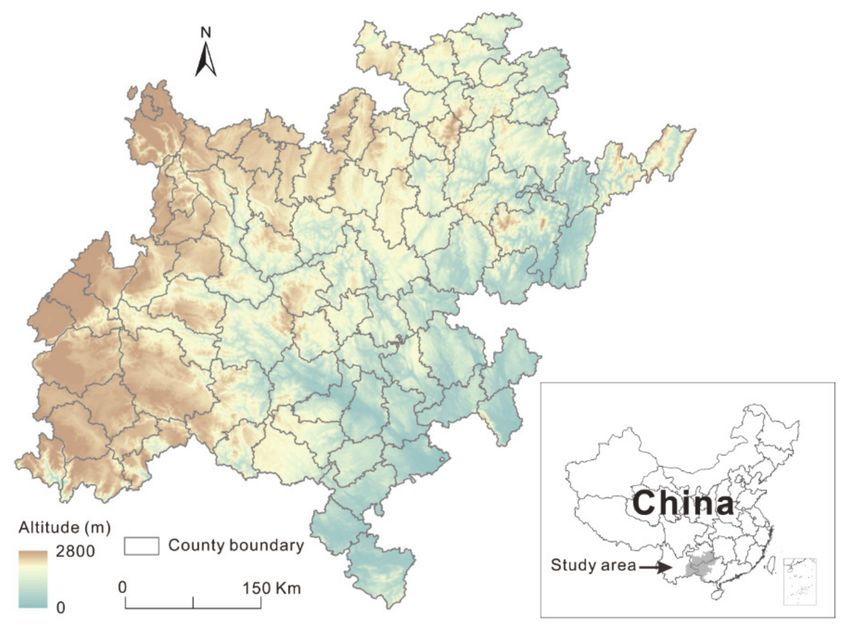
Sustainability 2021, 13, 8717                                                                                           2 of 14

                                important component of poverty studies, and the basis for scientifically formulating poverty
                                alleviation strategies [6]. Traditional poverty identification studies mainly rely on field
                                survey data or officially released statistical data to measure poverty [7–9]. Field survey is
                                time-consuming and labor-intensive and is also difficult to conduct at a large scale. Limited
                                numbers of surveying samples leads to large uncertainties [10]. The official statistical data
                                are generally collected by administrative districts and cannot accurately reflect the spatial
                                differences within administrative units. Satellite remote sensing, especially night-time light
                                (NTL) remote sensing, provides a new way for large-scale socioeconomic spatial monitoring
                                and evaluation [11]. The Defense Meteorological Satellite Program (DMSP)/Operational
                                Linescan System (OLS) data are the earliest NTL satellite data and have been widely used
                                for socioeconomic activity monitoring. However, DMSP/OLS has the shortcomings of
                                relatively coarse spatial resolution, low radiation resolution, lack of on-board calibration,
                                and signal saturation in urban centers [12]. The new generation NTL satellite data, Suomi
                                National Polar-orbiting Partnership (NPP)/Visible Infrared Imaging Radiometer Suite
                                (VIIRS), was put into use in 2012. Compared with DMSP/OLS, NPP/VIIRS has significantly
                                improved spatial resolution, quantization, dynamic range, and calibration [13]. Studies
                                have shown that there is a close relationship between NTL satellite data and regional
                                economic development [14,15]. NTL satellite data has been widely used in studies on
                                urban expansion [16–18], economic evaluation [19,20], population estimation [21–23], and
                                power consumption [24,25].
                                      The NTL satellite data also has potential in poverty assessment. However, there are
                                relatively few studies on poverty monitoring by NTL data. Ebener et al. [26] estimated
                                the distribution of income per capita as the proxy for wealth at the country and sub-
                                national level based on DMSP/OLS NTL data and population data, and analyzed its
                                relationship with health indicators. Noor et al. [27] calculated the asset-based poverty
                                index of 338 level-1 administrative districts in 37 African countries based on household
                                survey data and analyzed their relationship with DMSP/OLS data, indicating that NTL is
                                an effective alternative for the poverty survey data. Elvidge et al. [28] produced a global
                                poverty map using a poverty index by dividing LandScan population count by the average
                                values of DMSP/OLS NTL data, and also estimated the percentage of the population
                                living in poverty using a univariate linear model. Wang et al. [29] calculated an integrated
                                poverty index (IPI) at the provincial scale in China based on 17 socioeconomic indicators
                                using principal component analysis and then used regression analysis to explore the
                                relationship between IPI and the average light index (ALI) of DMPS/OLS data, achieving
                                an R2 of 0.854. Yu et al. [30] combined 10 socioeconomic indicators to calculate the IPI
                                of the 38 counties of Chongqing, China, and verified the relationship between IPI and
                                ALI using linear regression. The validation result showed an R2 of 0.86, suggesting good
                                correlation between them. Njuguna and McSharry [31] estimated the multi-dimensional
                                poverty index (MPI) at the sector level in Rwanda based on VIIRS NTL data, Landscan
                                population data, and detailed call records using multivariate regression, achieving a cross-
                                validated correlation coefficient of 0.88. Pan et al. [32] developed a linear regression model
                                to estimate MPI from NPP/VIIRS ALI in Chongqing Municipality, China, and tested the
                                developed model in Shaanxi Province, showing an average relative error of 11.12%. The
                                developed model was applied to map poverty in China at the county scale. The above
                                studies mainly used correlation and univariate linear regression analysis to establish the
                                quantitative relationship between poverty and NTL. However, due to the complexity and
                                diversity of the causes and manifestations of poverty, the relatively simple one-factor
                                linear model is insufficient to fit the relationship between poverty and light intensity. Li
                                et al. [33] classified high-poverty counties in China based on the features extracted from
                                DMSP/OLS NTL data using seven machine learning approaches (Gaussian process with
                                radial basis function kernel, stochastic gradient boosting, partial least squares regression
                                for generalized linear models, random forest, rotation forest, support vector machine,
                                and neural network with feature extraction). The overall accuracies of all models were
                                higher than 82%, suggesting that machine learning algorithms can effectively identify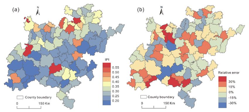
Sustainability 2021, 13, 8717                                                                                         3 of 14

                                high-poverty counties. Zhao et al. [34] used the random forest method to estimate the
                                household wealth index (HWI) of Bangladesh based on the spatial features extracted
                                from NPP/VIIRS NTL data, Google satellite images, land cover, road maps, and division
                                headquarter location data. The validation results showed an R2 of 0.70 in Bangladesh and
                                an R2 of 0.61 in Nepal. Shi et al. [35] developed a comprehensive poverty index (CPI) in
                                Chongqing, China by combining NPP/VIIRS NTL data, DEM, the normalized differential
                                vegetation index (NDVI) and point of interest (POI) data. The developed CPI was validated
                                by visual comparisons with Google Earth images and poverty-stricken villages, showing
                                good fitness between CPI and them. CPI values were also compared with MPI values at
                                the county level, achieving an R2 of 0.931. Li et al. [36] calculated a farmer sustainable
                                livelihood index (FSLI) from socioeconomic indicators to measure county-level poverty in
                                Hubei province. First-order and second-order linear regression were performed to estimate
                                FSLI from Luojia 1-01 ALI, achieving an R2 of 0.85 and 0.88, respectively. Yin et al. [37]
                                classified poverty areas in Guizhou, China based on the spatial features extracted from
                                NPP/VIIRS NTL and geographical data using random forest, support vector machine,
                                and artificial neural networks. Random forest outperformed the other two methods with
                                an overall accuracy of 0.94. Niu et al. [38] estimated the multi-source data poverty index
                                (MDPI) in Guangzhou, China based on the spatial variables derived from NPP/VIIRS NTL,
                                Landsat8 image, POI, and housing rent data using the random forest algorithm, yielding
                                a correlation coefficient of 0.954. The recent poverty studies based on remote sensing
                                introduced more spatial variables and employed machine learning technology, showing
                                better performances than the traditional univariate linear regression methods. However,
                                various machine learning algorithms were mostly used for classifying poverty areas. For
                                quantitatively identifying poverty index, only random forest algorithm was used, while
                                other machine learning methods were still rarely used. In addition, relatively few studies
                                were conducted in contiguous extremely poor areas, the most important regions for poverty
                                alleviation in China.
                                      In this study, we aim to map poverty in the Dian-Gui-Qian contiguous extremely poor
                                area in southwest China based on multi-source spatial datasets using several machine
                                learning algorithms. The Dian-Gui-Qian contiguous extremely poor area is one of the most
                                important extremely contiguous poor areas in China and is characterized by complicated
                                social and natural conditions, making it a key area for poverty identification. The IPI
                                values were calculated at the county scale by integrating 13 socioeconomic indicators as the
                                dependent variables and various spatial features derived from multi-source geospatial data
                                were used as independent variables. To develop the best model for poverty identification,
                                eight machine learning algorithms were employed and compared using cross validation.
                                The model with best performance was applied to spatial input variables to map poverty
                                in the study area. The remotely sensed poverty map measures poverty on a fine spatial
                                scale and provides a reference for the formulation and implementation of the strategies for
                                targeted poverty alleviation in the study area, and the study provides a practical way for
                                identifying and evaluating the spatial pattern of poverty.

                                2. Study area and data
                                2.1. Study Area
                                     The Dian-Gui-Qian contiguous extremely poor area is located in southwest China
                                (Figure 1). It covers a total area of 227,544 km2 and has a permanent population of
                                29.15 million. There are 91 county-level administrative districts in this region, including
                                six municipal districts, five county-level cities, 66 counties, and 14 minority autonomous
                                counties. In China, administrative districts are divided into four levels: provincial (mu-
                                nicipality, province, autonomous region, and special administrative region), prefectural
                                (prefecture-level city, autonomous prefecture, prefecture, and league), county (district,
                                county-level city, county, autonomous county, banner, autonomous banner, special district,
                                forest district), and township (subdistrict, town, township, ethnic township, sum, ethnic
                                sum, and county-controlled district).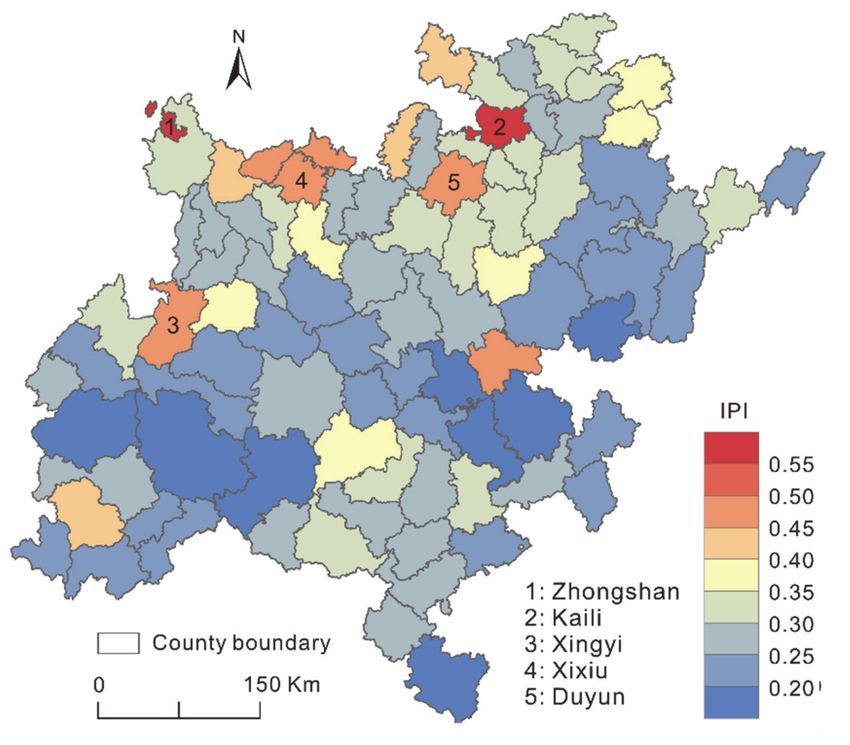
Sustainability 2021, 13, 8717                                                                                           4 of 14

                                Figure 1. Map of the study area and its location.

                                     The Dian-Gui-Qian contiguous extremely poor area is one of the most typical karst
                                areas in the world, whose landforms are mainly plateaus and mountains. Due to the
                                remote geographical location, harsh natural conditions, frequent natural disasters, and
                                weak infrastructure, the poverty problem in this region is serious. Among the 14 extremely
                                contiguous poor areas in China, this region has the largest number of counties, the most
                                poverty alleviation targets, and the largest ethnic minority population, making it a key area
                                of poverty alleviation.

                                2.2. Data
                                      The data used in this study mainly include county-level socioeconomic statistical data
                                and remote sensing data.
                                      The county-level socioeconomic statistical data was mainly collected from the China
                                County Statistical Yearbook of 2017, which provides socioeconomic statistical data in 2016.
                                The supplemented socioeconomic statistical material included the statistical yearbooks of
                                the cities and the statistical bulletins on national economic and social development in the
                                study area.
                                      The remote sensing data include NPP/VIIRS NTL data, SRTM DEM data, Finer
                                Resolution Observation and Monitoring Global land cover (FROM-GLC) data, open street
                                map (OSM) data, accessibility to cities, and natural disaster data.
                                      NPP/VIIRS NTL data were the NPP/VIIRS DNB annual cloud-free composite data in
                                2016 provided by the National Oceanic and Atmospheric Administration (NOAA) Earth
                                Observation Group. This data provides annual average radiance by excluding the influence
                                of stray light, lightning, lunar illumination, cloud-cover and temporal lights, with a spatial
                                resolution of 15 arc-seconds (~500 m).
                                      The FROM-GLC land cover data in 2015 were provided by the Department of Earth
                                Sciences at Tsinghua University. FROM-GLC is a 30 m resolution global land cover prod-
                                uct developed by a random forest-based mapping framework based on Landsat remote
                                sensing data. The classification scheme contains 11 land cover categories: cropland, forest,
                                grassland, shrubland, wetland, water, tundra, impervious surface, bareland, snow/ice,
                                and cloud.
                                      OSM is a free editable map amended by volunteers from all over the world, providing
                                geospatial information such as roads, buildings, and water bodies. The road network in
                                the study area was extracted from OSM database.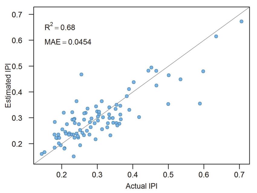
Sustainability 2021, 13, 8717                                                                                             5 of 14

                                     The DEM data used in this study were the SRTM DEM data provided by the United
                                States Geological Survey (USGS) with a spatial resolution of 1 arc-second (~30 m).
                                     Accessibility to cities data, provided by the Malaria Atlas Project, is a global map
                                of travel time to cities in 2015. It quantifies travel time to cities at a spatial resolution of
                                30 arc-seconds (~1 km) by integrating spatial variables that affect human movement rates
                                such as roads, railways, land covers, topographical conditions and national borders [39].
                                     Natural disaster data was derived from the global estimated risk index provided by
                                the Global Risk Data Platform. The index at a spatial resolution of 5 arc-minutes (~10 km)
                                was estimated from multiple hazards including tropical cyclone, flood, and landslide
                                induced by precipitations, with the index value ranges from 1 (low) to 5 (extreme).

                                3. Methods
                                3.1. IPI Calculation from Census Data
                                     Poverty is a comprehensive social phenomenon that is not only related to income and
                                assets but is also closely related to factors such as health and education. Simply using a
                                single indicator cannot fully reflect the poverty situation. Some studies have proposed to
                                quantify poverty by combing a collection of socioeconomic indicators. In this study, IPI
                                was used to indicate poverty conditions. According to previous research, IPI was calcu-
                                lated from multiple socioeconomic indicators, which cover economic development, living
                                conditions, health, and education. In total, 13 socioeconomic indicators were employed to
                                calculate IPI (Table 1).

                                Table 1. Measurement indicators of IPI.

                                      Dimension                           Indicator                   Attribute    Weight
                                                                    Per capita GDP                    Positive      0.0645
                                      Economic
                                                             Per capita fiscal expenditure            Positive      0.0457
                                     development
                                                                  Per capita savings                  Positive      0.0881
                                                                  Per capita income                   Positive      0.0627
                                                                Per capita fixed assets               Positive      0.1727
                                   Living conditions
                                                           Endowment insurance coverage               Positive      0.0361
                                                              Per capita telephone ratio              Positive      0.1006
                                                               Per capita beds in health              Positive      0.1151
                                        Health                    Per capita doctors                  Positive      0.0481
                                                             Medical insurance coverage               Positive      0.0135
                                                            Per capita students present in
                                                                                                      Positive      0.1220
                                                              primary and high schools
                                       Education
                                                          Per capita teachers at primary and
                                                                                                      Positive      0.0589
                                                                      high schools
                                                          Per capita education expenditure            Positive      0.0722

                                    To eliminate the dimension differences of different indicators, each indicator was
                                min–max normalized:
                                                                      xij − min( xi )
                                                             Xij =                                                  (1)
                                                                    max( xi ) − min( xi )
                                where Xij is the normalized value of the jth sample of indicator i, xij is the original value
                                of the jth sample of indicator i, and min(xi ) and max(xi ) are the minimum and maximum
                                values of the ith indicator, respectively.
                                     The weight of each indicator was determined using the entropy weight method to
                                avoid the bias caused by subjective factors. For an indicator, higher information entropy
                                indicates greater role of this indicator in the comprehensive evaluation.
                                     The entropy of indicator i (ei ) was calculated as follows:
                                                                                       n
                                                                ei = − ln(n)−1 · ∑ Pij · ln Pij

                                                                                                                             (2)
                                                                                      i =1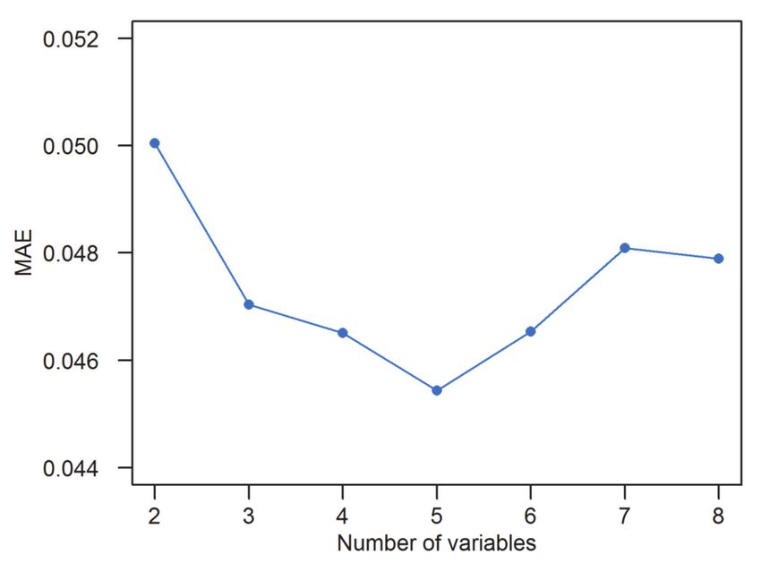
Sustainability 2021, 13, 8717                                                                                            6 of 14

                                where n is the number of samples, and:

                                                                                       Xij
                                                                            Pij =    n                                      (3)
                                                                                    ∑ j=1 Xij

                                     The deviation degree of indicator i (di ) was calculated as follows:

                                                                             d i = 1 − ei                                   (4)

                                     The weight of indicator i (wi ) was calculated as follows:

                                                                                       di
                                                                            wi =                                            (5)
                                                                                    ∑im=1 di

                                where m is the number of predictors.
                                    The calculated weights of the indicators are shown in Table 1. Then, the IPI of each
                                county-level administrative district was calculated as follows:
                                                                                     m
                                                                        IPIj =      ∑ Xij ·wi                               (6)
                                                                                    i =1

                                where IPIj is the IPI value of the jth sample. A high IPI value indicates a low level of
                                poverty, while a low IPI value refers to a high level of poverty.

                                3.2. IPI Identification from Spatial Data
                                      Poverty is a complex phenomenon, which should be understood from multi-source
                                data to improve the accuracy of poverty mapping [40]. In this study, a number of spatial
                                independent variables were extracted from multi-source geospatial data for the spatial
                                identification of poverty. The average NTL was extracted from the NPP/VIIRS data, the
                                traffic accessibility (TA) was extracted from the city accessibility data, the altitude (H) was
                                extracted from the SRTM/DEM data, the flat area (slope < 5◦ ) coverage (FAC) was derived
                                from the SRTM/DEM data, the impervious surface coverage (ISC) and cropland coverage
                                (CC) were calculated from the FROM-GLC data, the road density (RD) was calculated
                                based on the OSM road network data, and the risk index (RI) was extracted from the
                                globally estimated risk index data. A total of eight independent variables are used for the
                                spatial identification of poverty: NTL, H, FAC, ISC, CC, TA, RD, and RI.
                                      Considering the different natural and socioeconomic conditions in different regions
                                and the complex relationships between various factors, the relationships between the
                                poverty level and independent spatial variables in different regions may be different. In
                                addition to the traditional multiple linear regression (MLR), machine learning methods
                                such as the bidirectional recurrent neural network (BRNN), generalized additive model
                                (GAM), support vector machine (SVM), MARS, random forest (RF), XGBoost, and Cubist,
                                were also employed to estimate the IPI from independent spatial variables. Compared
                                with the MLR, machine learning models have the advantage of being able to fit complex,
                                high-dimensional nonlinear relationships [41].
                                      Ten-fold cross-validation (CV) was used to verify model performance. The whole
                                dataset was randomly divided into ten folds, one of which was used as the test dataset
                                and the other nine folds were used as the training dataset. This process was repeated
                                10 times so that all samples were used once as validation samples. In the CV process, the
                                parameters of each model are tested to optimize the model, and the parameters that obtain
                                the minimum error are used to fit the final model. The mean absolute error (MAE) and
                                coefficient of determination (R2 ) are calculated and used as accuracy evaluation indicators.
                                The method with the highest accuracy is used to establish the final IPI estimation model.
                                      To reduce the overfitting problem of machine learning models, feature selection was
                                performed to control the complexity of the model. The eight variables were screened to
                                determine the optimal variable combination. First, all the combinations of two variables
Sustainability 2021, 13, 8717                                                                                                    7 of 14

                                were tested to determine the combination with the highest accuracy. Then, a new inde-
                                pendent variable was added to fit the model. The new independent variable with the
                                best performance was retained. By analyzing the influence of adding new variables to the
                                model performance, the optimal robust combination of variables was determined.
                                      When the final model was developed, the importance of each variable was quantified
                                to evaluate the contributions of each independent variable to the IPI estimation. For each
                                variable, the percentage increase in MAE (% IncMAE) was calculated as the measure
                                of its importance when the variable was randomly permuted and the other variables
                                remained unchanged.

                                4. Results
                                4.1. Relationship between IPI and NTL
                                     Based on the values and corresponding weights of the 13 socioeconomic indicators
                                of the 91 county-level administrative districts in the study area, the IPI values of these
                                administrative districts were calculated. The Luocheng Mulao Autonomous County has
                                the lowest IPI of 0.1436, and the Kaili County-level City has the highest IPI of 0.7057. For
                                all administrative districts, the average IPI is 0.3045, the median IPI is 0.2792, and the
                                skewness is 1.357. The majority of administrative districts show lower IPI values than the
                                average value.
                                     Previous studies have shown that NTL data is an effective spatial indicator of poverty.
                                Figure 2 shows the scatterplots between the NTL and IPI values of the 91 county-level
                                administrative districts. A correlation coefficient (R) of 0.63 indicates that there was a
                                positive but not strong correlation between them. The NTL values of most administrative
                                districts were relatively low (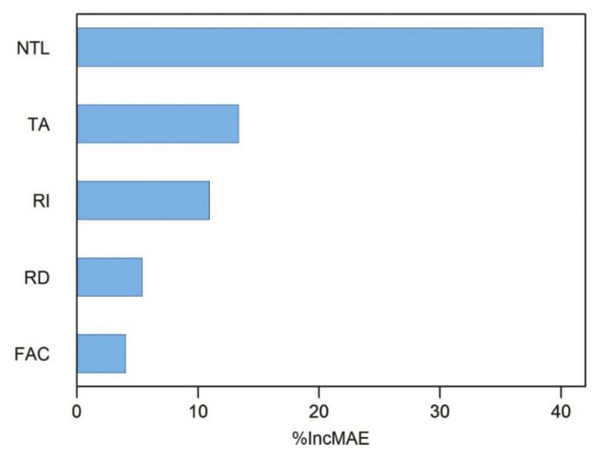
Sustainability 2021, 13, 8717                                                                                         8 of 14

                                relationship between the IPI and independent variables very well. The XGBoost model
                                had the highest accuracy (MAE = 0.0479, R2 = 0.61) and therefore was selected as the final
                                model to map IPI from spatial variables.

                                Table 2. Accuracies of the nine models.

                                             Model                          MAE                            R2
                                              MLR                          0.0767                         0.23
                                             BRNN                          0.0593                         0.47
                                             GAM                           0.0498                         0.59
                                              SVM                          0.0583                         0.49
                                             MARS                          0.0581                         0.46
                                               RF                          0.0527                         0.57
                                            XGBoost                        0.0479                         0.61
                                             Cubist                         0.054                         0.53

                                     Forward feature selection was applied in the XGBoost modelling to develop a simple
                                model with fewer variables to reduce overfitting. Figure 3 shows the variations of minimum
                                MAE with the number of variables. As the number of variables increased from 1 to 5, the
                                model error significantly decreased. Then, as the number of variables continued to increase,
                                the error tended to increase. Therefore, the combination of five variables (NTL, TA, RI, RD,
                                and FAC) was used to develop the XGBoost model for IPI estimation.

                                Figure 3. Variation of minimum MAE with the number of variables.

                                     Figure 4 shows the scatterplot between the actual IPI and the IPI estimated by the
                                XGBoost model, which is constructed based on the selected five variables. The MAE is
                                0.0454, and R2 is 0.68. Most samples were clustered near the 1:1 line, indicating that the
                                predicted IPI values were in good agreement with the actual IPI values. Wealthy county-
                                level administrative districts (IPI > 0.5) were slightly underestimated, and other samples
                                were not obviously overestimated or underestimated. In addition, the fitting error did not
                                vary with the IPI value, indicating no heteroscedasticity problem.
Sustainability 2021, 13, 8717 9 of 14
Figure 4. Scatterplot between the actual and estimated IPI values of county-level administrative districts.
Figure 5 shows the influence of the five variables on the XGBoost model. NTL had the
highest importance (% IncMAE = 38.51%), indicating that NTL was the most important
variable for capturing the spatial variance in poverty. NTL can effectively reflect the
intensity of human activities and is closely related to the social economy, thus resulting in a
very high importance index. The importance of TA (% IncMAE = 13.33%) was secondary to
that of NTL, suggesting that the connection to cities in the study area restricted the economic
development to a great extent. RI also had a high importance (% IncMAE = 10.03%),
indicating that natural disasters in this region were also an important factor restricting
residential poverty levels. The % IncRMSE values of RD and FAC were 5.38% and 4.01%,
respectively, indicating that local traffic and terrain conditions had a certain influence on
the level of poverty, but such influence was less than that of the other three variables.
Figure 5. Importance of the input variables in the XGBoost model.
4.3. Spatial Distribution of IPI
The validation results suggested that the XGBoost model developed based on five
variables (NTL, TA, RI, RD, and FAC) was the best model for poverty mapping in the
Dian-Gui-Qian contiguous extremely poor area. Figure 6 shows the spatial distribution
of the estimated county-level IPI derived from the XGBoost model. Generally, the overall
IPI values of northern parts were obviously higher than those of southern regions. The
wealthy regions with high IPI values were mainly prefectural districts and county-level
cities, such as Zhongshan District, Kaili County-level City, Xingyi County-level City, Xixiu
District, and Duyun County-level City (labeled in the figure). These regions had relativelySustainability 2021, 13, 8717 10 of 14
good socioeconomic foundations, decent infrastructure, and well developed industry and
commerce, making the poverty level relatively low in these county-level districts. The
poor regions with low IPI values were mainly located in the southwest and east of the
study area. These regions had poor transportation, ethnic minority settlements, irrational
industrial structures, and weak social and economic foundations, leading to deep poverty.
Figure 6. Spatial distribution of the remotely sensed county-level IPI derived from the XGBoost
model. The typical county-level administrative units are labeled with numbers.
To assess the reliability of the spatial distribution of the remotely sensed county-level
IPI map, it was compared with the actual county-level IPI map (Figure 7a). Similar to
Figure 6, the actual IPI map also shows a high pattern in the north and low pattern in the
south, suggesting good spatial prediction of the remotely sensed poverty. The relative
errors of all county-level districts were also calculated (Figure 7b). Most of the county-level
districts showed relative errors within ±15%, and only a few county-level districts had
relative errors higher than 30% or lower than −30%. The spatial assessment indicates that
the remotely sensed IPI map can effectively characterize the spatial distribution of poverty.
It was also noted that the county-level districts with high IPI values generally showed
negative relative errors, suggesting that the remotely sensed IPI values were less than the
actual IPI values. This phenomenon indicated the slight underestimation of the wealthy
regions in the remotely sensed result, as pointed out in the aforementioned analysis.
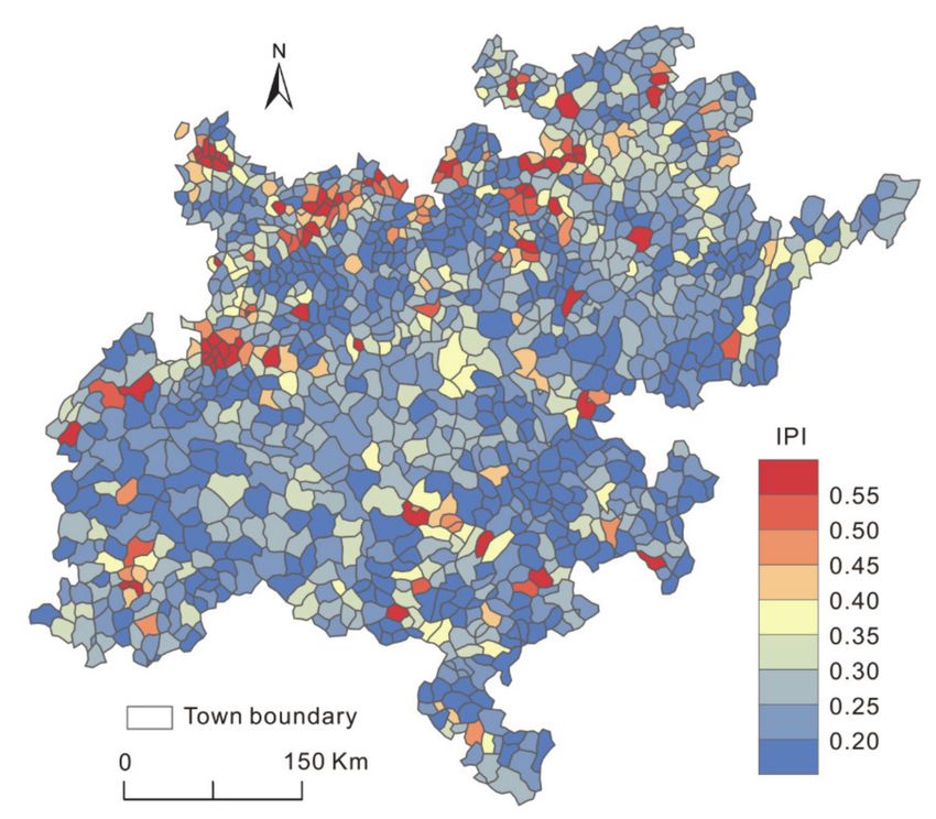
Based on the developed XGBoost model and the spatial variables, the distribution
of IPI at town level in the study area was also mapped (Figure 8). Because of lacking
town-level socioeconomic statistical data, the remotely sensed town-level IPI map cannot
be quantitatively validated, but can be compared with the county-level IPI map to assess
the spatial consistency between them. Compared to the county-level IPI map, the town-
level IPI map showed a similar overall distribution pattern that most wealthy units were
located in the northern part. However, the township-level IPI map reflected more detailed
spatial differences. In the northern part of the study area, there were many wealthy town-
level administrative districts (IPI > 0.45), but there were also some very poor town-level
districts (IPI < 0.25), indicating strong inequality in this area. The town-level administrative
districts in the southern part generally showed low IPI values, and the gap in wealth was
relatively small. These detailed spatial patterns cannot be reflected by the county-level IPI
map but can be well identified by the town-level IPI map. The developed remote sensing
model for IPI estimation can also be applied at a finer scale, such as the village-levelSustainability 2021, 13, 8717 11 of 14
administrative districts or pixels, to reveal more detailed information about the spatial
distribution of poverty.
Figure 7. Spatial distribution of the actual county-level IPI (a) and relative error (b) in the Dian-Gui-
Qian contiguous poor area.
Figure 8. Spatial distribution of the remotely sensed town-level IPI in the Dian-Gui-Qian contiguous
poor area.
5. Discussion
Compared with previous studies, the correlation coefficient between poverty and NTL
in the Dian-Gui-Qian contiguous extremely poor area is quite low (R = 0.63) in this study.
This may be attributed to the complex terrain in the study area and the large differences
between the natural and economic conditions of the administrative districts. Due to the low
correlation between IPI and NTL, it is difficult to achieve ideal results by simple regression
models with NTL as the only independent variable. Therefore, auxiliary spatial variables
shall be introduced to improve the accuracy. Under this consideration, terrain, land
cover, traffic, and raster variables were also included. Given the complicated relationships
between poverty and these spatial variables, several machine learning algorithms were
employed to fit the relationships between poverty and spatial variables. Considering that
linear regression was widely used in previous studies, a MLR model was also developed
as a comparison. The validation results indicated that machine learning models, especiallySustainability 2021, 13, 8717 12 of 14
the ensemble learning models such as XGBoost, achieved much higher accuracies than the
MLR model. This study indicates that machine learning algorithms based on multi-source
spatial data can effectively identify the spatial distribution of poverty, providing a reliable
way to map poverty in regions with complex natural and socioeconomic conditions. All
the spatial datasets used in this study can be timely and freely obtained. Therefore, the
proposed method can be conveniently applied in other areas for poverty mapping without
being constrained by data acquisition.
Although the method in this study shows efficiency for poverty mapping, there are
still some limitations. Poverty is a complicated issue related to various socioeconomic
conditions. This paper introduced multi-source spatial variables to identify poverty. How-
ever, most of the spatial variables are environmental indicators that can just indirectly
reflect poverty. In addition, it should be noted that with the development of information
technology, new economic forms such as the internet economy have broken through the
limitation of geographic space. The associated factors of wealth have become increasingly
complex and diverse, and their spatial identifications are therefore facing greater challenges.
Nighttime light remote sensing data provide a unique way to monitor human activities
from space at night, making it a useful indicator to identify poverty. In this study, NTL
derived from NPP/VIIRS showed the highest importance for poverty mapping. However,
the spatial resolution of NPP/VIIRS is not very high, which may not effectively reflect
spatial details of human activity patterns. Moreover, due to the lack of household survey
data, further validation cannot be performed at a finer scale in this study. If sufficient
household survey data can be collected, the method proposed in this paper will be more
comprehensively validated on a small scale.
6. Conclusions
The capability of machine learning technology on poverty mapping from multiple
remote sensing data has been evaluated in this paper. The IPI was calculated from the
socioeconomic indicators of county-level administrative districts in the Dian-Gui-Qian
contiguous extremely poor area of southwest China. Then, multiple spatial indicators
were extracted from NTL, DEM, land cover, OSM, city accessibility, and natural disaster
data as the spatial variables for poverty mapping. Several machine learning algorithms
were employed and compared to develop models for estimating county-level IPI over the
study area. Cross validation results suggested that XGBoost outperformed other methods
and exhibited the best performance. By feature selection, the final XGBoost model was
developed, which achieved an MAE of 0.0454 and an R2 of 0.68.
The spatial pattern of the remotely sensed county-level IPI map is similar to that of the
actual IPI map, indicating that it can effectively characterize the spatial pattern of poverty.
By applying the developed model to spatially independent variables, an IPI map at a
finer resolution could be produced, such as town-level or even pixel-level. The remotely
sensed IPI provides a valuable reference for a more detailed understanding of the poverty
situation in the Dian-Gui-Qian contiguous poor area, which is helpful for the formulation
and implementation of the government’s targeted poverty alleviation strategy.
In the future, some efforts could be considered to improve the spatial identification of
poverty: Additional spatial datasets, especially the datasets that have direct relationships
with poverty should be employed to quantify poverty from a more comprehensive perspec-
tive, including POI, location-based social media data, and mobile signaling data; nighttime
light remote sensing data with higher spatial resolution, such as Luojia 1-01, can be used to
provide more details of human activities for poverty mapping. Deep learning technology
is expected to extract detailed building information from high resolution satellite images,
which is an important and complementary spatial variable for poverty identification.
Author Contributions: Conceptualization, Y.X.; methodology, Y.X.; software, Y.X. and Y.M.; formal
analysis, Y.M.; resources, Y.X. and S.Z.; writing—original draft preparation, Y.X.; writing—review
and editing, Y.M., Y.M., and S.Z.; project administration, Y.X., funding acquisition, Y.X. and S.Z. All
authors have read and agreed to the published version of the manuscript.Sustainability 2021, 13, 8717 13 of 14
Funding: This research was funded by the Humanities and Social Sciences Foundation of the Ministry
of Education of China (17YJCZH205) and the Qing Lan Project of Jiangsu Province (R2019Q03).
Institutional Review Board Statement: Not applicable.
Informed Consent Statement: Not applicable.
Acknowledgments: The authors would like to thank the National Bureau of Statistics of China for
providing statistical data, the National Oceanic and Atmospheric Administration (NOAA) Earth
Observation Group (EOG) for providing NPP/VIIRS nighttime data, the US Geological Survey
(USGS) for providing SRTM/DEM data, the Department of Earth Sciences at Tsinghua University
for providing FROM-GLC data, OpenStreetMap for providing geospatial information data, the
Malaria Atlas Project for providing Accessibility to cities data, and the Global Risk Data Platform for
providing the global estimated risk index data.
Conflicts of Interest: The authors declare no conflict of interest.
References
1. Braithwaite, A.; Dasandi, N.; Hudson, D. Does Poverty Cause Conflict? Isolating the Causal Origins of the Conflict Trap. Confl.
Manag. Peace Sci. 2016, 33, 45–66. [CrossRef]
2. Cf, O. Transforming Our World: The 2030 Agenda for Sustainable Development; United Nations: New York, NY, USA, 2015.
3. Office of Household Survey, National Bureau of Statistics of China. Report on Rural Poverty in China 2018; China Statistics Press:
Beijing, China, 2018. (In Chinese)
4. Liu, H. Study on Implementation of Targeted Poverty Alleviation and Regional Coordinated Development. Bull. Chin. Acad. Sci.
2016, 31, 320–327. (In Chinese)
5. Ding, J. Comparative Analysis on Poverty Degree of China’s 11 Contiguous Destitute Areas: With View of Comprehensive
Development Index. Sci. Geogr. Sin. 2014, 34, 1418–1427. (In Chinese)
6. Sachs, J.D.; Mellinger, A.D.; Gallup, J.L. The Geography of Poverty and Wealth. Sci. Am. 2001, 284, 70–75. [CrossRef]
7. Elbers, C.; Lanjouw, J.O.; Lanjouw, P. Micro-Level Estimation of Poverty and Inequality. Econometrica 2003, 71, 355–364. [CrossRef]
8. Hentschel, J.; Lanjouw, J.O.; Lanjouw, P.; Poggi, J. Combining Census and Survey Data to Trace the Spatial Dimensions of Poverty:
A Case Study of Ecuador. World Bank Econ. Rev. 2000, 14, 147–165. [CrossRef]
9. Lanjouw, P.; Marra, M.; Nguyen, C. Vietnam’s Evolving Poverty Index Map: Patterns and Implications for Policy. Soc. Indic. Res.
2017, 133, 93–118. [CrossRef]
10. Jean, N.; Burke, M.; Xie, M.; Davis, W.M.; Lobell, D.B.; Ermon, S. Combining Satellite Imagery and Machine Learning to Predict
Poverty. Science 2016, 353, 790–794. [CrossRef] [PubMed]
11. Ghosh, T.; Anderson, S.J.; Elvidge, C.D.; Sutton, P.C. Using Nighttime Satellite Imagery as a Proxy Measure of Human Well-Being.
Sustainability 2013, 5, 4988–5019. [CrossRef]
12. Elvidge, C.D.; Cinzano, P.; Pettit, D.R.; Arvesen, J.; Sutton, P.; Small, C.; Nemani, R.; Longcore, T.; Rich, C.; Safran, J. The Nightsat
Mission Concept. Int. J. Remote Sens. 2007, 28, 2645–2670. [CrossRef]
13. Elvidge, C.D.; Baugh, K.E.; Zhizhin, M.; Hsu, F.-C. Why VIIRS Data Are Superior to DMSP for Mapping Nighttime Lights. Proc.
Asia-Pac. Adv. Netw. 2013, 35, 62. [CrossRef]
14. Elvidge, C.D.; Baugh, K.E.; Kihn, E.A.; Kroehl, H.W.; Davis, E.R.; Davis, C.W. Relation between Satellite Observed Visible-near
Infrared Emissions, Population, Economic Activity and Electric Power Consumption. Int. J. Remote Sens. 1997, 18, 1373–1379.
[CrossRef]
15. Li, D.; Zhao, X.; Li, X. Remote Sensing of Human Beings—A Perspective from Nighttime Light. Geo-Spat. Inf. Sci. 2016, 19, 69–79.
[CrossRef]
16. Ma, T.; Zhou, Y.; Zhou, C.; Haynie, S.; Pei, T.; Xu, T. Night-Time Light Derived Estimation of Spatio-Temporal Characteristics of
Urbanization Dynamics Using DMSP/OLS Satellite Data. Remote Sens. Environ. 2015, 158, 453–464. [CrossRef]
17. Zhou, Y.; Li, X.; Asrar, G.R.; Smith, S.J.; Imhoff, M. A Global Record of Annual Urban Dynamics (1992–2013) from Nighttime
Lights. Remote Sens. Environ. 2018, 219, 206–220. [CrossRef]
18. Alahmadi, M.; Atkinson, P.M. Three-Fold Urban Expansion in Saudi Arabia from 1992 to 2013 Observed Using Calibrated
DMSP-OLS Night-Time Lights Imagery. Remote Sens. 2019, 11, 2266. [CrossRef]
19. Sutton, P.; Roberts, D.; Elvidge, C.; Baugh, K. Census from Heaven: An Estimate of the Global Human Population Using
Night-Time Satellite Imagery. Int. J. Remote Sens. 2001, 22, 3061–3076. [CrossRef]
20. Doll, C.N.; Muller, J.-P.; Morley, J.G. Mapping Regional Economic Activity from Night-Time Light Satellite Imagery. Ecol. Econ.
2006, 57, 75–92. [CrossRef]
21. Briggs, D.J.; Gulliver, J.; Fecht, D.; Vienneau, D.M. Dasymetric Modelling of Small-Area Population Distribution Using Land
Cover and Light Emissions Data. Remote Sens. Environ. 2007, 108, 451–466. [CrossRef]
22. Sun, W.; Zhang, X.; Wang, N.; Cen, Y. Estimating Population Density Using DMSP-OLS Night-Time Imagery and Land Cover
Data. IEEE J. Sel. Top. Appl. Earth Obs. Remote Sens. 2017, 10, 2674–2684. [CrossRef]Sustainability 2021, 13, 8717 14 of 14
23. Tan, M.; Li, X.; Li, S.; Xin, L.; Wang, X.; Li, Q.; Li, W.; Li, Y.; Xiang, W. Modeling Population Density Based on Nighttime Light
Images and Land Use Data in China. Appl. Geogr. 2018, 90, 239–247. [CrossRef]
24. Chand, T.K.; Badarinath, K.V.S.; Elvidge, C.D.; Tuttle, B.T. Spatial Characterization of Electrical Power Consumption Patterns
over India Using Temporal DMSP-OLS Night-Time Satellite Data. Int. J. Remote Sens. 2009, 30, 647–661. [CrossRef]
25. Shi, K.; Yu, B.; Huang, C.; Wu, J.; Sun, X. Exploring Spatiotemporal Patterns of Electric Power Consumption in Countries along
the Belt and Road. Energy 2018, 150, 847–859. [CrossRef]
26. Ebener, S.; Murray, C.; Tandon, A.; Elvidge, C.C. From Wealth to Health: Modelling the Distribution of Income per Capita at the
Sub-National Level Using Night-Time Light Imagery. Int. J. Health Geogr. 2005, 4, 5. [CrossRef] [PubMed]
27. Noor, A.M.; Alegana, V.A.; Gething, P.W.; Tatem, A.J.; Snow, R.W. Using Remotely Sensed Night-Time Light as a Proxy for
Poverty in Africa. Popul. Health Metr. 2008, 6, 5. [CrossRef]
28. Elvidge, C.D.; Sutton, P.C.; Ghosh, T.; Tuttle, B.T.; Baugh, K.E.; Bhaduri, B.; Bright, E. A Global Poverty Map Derived from Satellite
Data. Comput. Geosci. 2009, 35, 1652–1660. [CrossRef]
29. Wang, W.; Cheng, H.; Zhang, L. Poverty Assessment Using DMSP/OLS Night-Time Light Satellite Imagery at a Provincial Scale
in China. Adv. Space Res. 2012, 49, 1253–1264. [CrossRef]
30. Yu, B.; Shi, K.; Hu, Y.; Huang, C.; Chen, Z.; Wu, J. Poverty Evaluation Using NPP-VIIRS Nighttime Light Composite Data at the
County Level in China. IEEE J. Sel. Top. Appl. Earth Obs. Remote Sens. 2015, 8, 1217–1229. [CrossRef]
31. Njuguna, C.; McSharry, P. Constructing Spatiotemporal Poverty Indices from Big Data. J. Bus. Res. 2017, 70, 318–327. [CrossRef]
32. Pan, J.; Hu, Y. Spatial Identification of Multi-Dimensional Poverty in Rural China: A Perspective of Nighttime-Light Remote
Sensing Data. J. Indian Soc. Remote Sens. 2018, 46, 1093–1111. [CrossRef]
33. Li, G.; Cai, Z.; Liu, X.; Liu, J.; Su, S. A Comparison of Machine Learning Approaches for Identifying High-Poverty Counties:
Robust Features of DMSP/OLS Night-Time Light Imagery. Int. J. Remote Sens. 2019, 40, 5716–5736. [CrossRef]
34. Zhao, X.; Yu, B.; Liu, Y.; Chen, Z.; Li, Q.; Wang, C.; Wu, J. Estimation of Poverty Using Random Forest Regression with
Multi-Source Data: A Case Study in Bangladesh. Remote Sens. 2019, 11, 375. [CrossRef]
35. Shi, K.; Chang, Z.; Chen, Z.; Wu, J.; Yu, B. Identifying and evaluating poverty using multisource remote sensing and point of
interest (POI) data: A case study of Chongqing, China. J. Clean. Prod. 2020, 255, 120245. [CrossRef]
36. Li, C.; Yang, W.; Tang, Q.; Tang, X.; Lei, J.; Wu, M.; Qiu, S. Detection of Multidimensional Poverty Using Luojia 1-01 Nighttime
Light Imagery. J. Indian Soc. Remote Sens. 2020, 48, 963–977. [CrossRef]
37. Yin, J.; Qiu, Y.; Zhang, B. Identification of Poverty Areas by Remote Sensing and Machine Learning: A Case Study in Guizhou,
Southwest China. Int. J. Geo-Inf. 2021, 10, 11. [CrossRef]
38. Niu, T.; Chen, Y.; Yuan, Y. Measuring urban poverty using multi-source data and a random forest algorithm: A case study in
Guangzhou. Sustain. Cities Soc. 2020, 54, 102014. [CrossRef]
39. Weiss, D.J.; Nelson, A.; Gibson, H.S.; Temperley, W.; Peedell, S.; Lieber, A.; Hancher, M.; Poyart, E.; Belchior, S.; Fullman, N. A
Global Map of Travel Time to Cities to Assess Inequalities in Accessibility in 2015. Nature 2018, 553, 333–336. [CrossRef] [PubMed]
40. Pokhriyal, N.; Jacques, D.C. Combining Disparate Data Sources for Improved Poverty Prediction and Mapping. Proc. Natl. Acad.
Sci. USA 2017, 114, E9783–E9792. [CrossRef]
41. Ngufor, C.; Murphree, D.; Upadhyaya, S.; Madde, N.; Kor, D.; Pathak, J. Effects of Plasma Transfusion on Perioperative Bleeding
Complications: A Machine Learning Approach. Stud. Health Technol. Inform. 2015, 216, 721. [PubMed]You can also read