Probabilistic Embeddings for Cross-Modal Retrieval - arXiv.org
←
→
Page content transcription
If your browser does not render page correctly, please read the page content below
Probabilistic Embeddings for Cross-Modal Retrieval
Sanghyuk Chun1 Seong Joon Oh1 Rafael Sampaio de Rezende2 Yannis Kalantidis2 Diane Larlus2
1 2
NAVER AI LAB NAVER LABS Europe
arXiv:2101.05068v1 [cs.CV] 13 Jan 2021
Abstract
Cross-modal retrieval methods build a common repre-
sentation space for samples from multiple modalities, typ-
ically from the vision and the language domains. For im-
ages and their captions, the multiplicity of the correspon-
dences makes the task particularly challenging. Given an
image (respectively a caption), there are multiple captions
(respectively images) that equally make sense. In this pa-
per, we argue that deterministic functions are not suffi-
ciently powerful to capture such one-to-many correspon-
dences. Instead, we propose to use Probabilistic Cross-
Modal Embedding (PCME), where samples from the differ-
ent modalities are represented as probabilistic distributions
in the common embedding space. Since common bench-
marks such as COCO suffer from non-exhaustive annota-
tions for cross-modal matches, we propose to additionally
evaluate retrieval on the CUB dataset, a smaller yet clean Figure 1. We propose to use probabilistic embeddings to rep-
database where all possible image-caption pairs are anno- resent images and their captions as probability distributions in a
tated. We extensively ablate PCME and demonstrate that common embedding space suited for cross-modal retrieval. These
it not only improves the retrieval performance over its de- distributions successfully model the uncertainty which results
terministic counterpart, but also provides uncertainty esti- from the multiplicity of concepts appearing in a visual scene and
mates that render the embeddings more interpretable. implicitly perform many-to-many matching between those con-
cepts.
1. Introduction
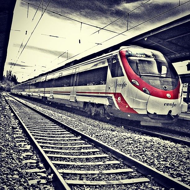
two of the choices from the COCO [6] annotators. Thus,
Given a query and a database from different modalities, the common representation has to deal with the fact that an
cross-modal retrieval is the task of retrieving the database image potentially matches with a number of different cap-
items which are most relevant to the query. Most research tions. Conversely, given a caption, there may be multiple
on this topic has focused on the image and text modali- manifestations of the caption in visual forms. The multiplic-
ties [6, 10, 27, 58]. Typically, methods estimate embedding ity of correspondences across image-text pairs stems in part
functions that map visual and textual inputs into a common from the different natures of the modalities. All the different
embedding space, such that the cross-modal retrieval task components of a visual scene are thoroughly and passively
boils down to the familiar nearest neighbour retrieval task captured in a photograph, while language descriptions are
in a Euclidean space [10, 52]. the product of conscious choices of the key relevant con-
Building a common representation space for multiple cepts to report from a given scene. All in all, a common
modalities is challenging. Consider an image with a group representation for image and text modalities is required to
of people on a platform preparing to board a train (Figure 1). model the one-to-many mappings in both directions.
There are more than one possible caption describing this Standard approaches which rely on vanilla functions do
image. “People waiting to board a train in a train platform” not meet this necessary condition: they can only quantify
and “The metro train has pulled into a large station” were one-to-one relationships [10, 52]. There have been attempts
1
to introduce multiplicity. For example, Song & Soley-                training on uni-modal triplets to preserve the structure in-
mani [47] have introduced the Polysemous Visual-Semantic             herent for each modality in the joint space. Faghri et al. [10]
Embeddings (PVSE) by letting an embedding function pro-              propose to learn such space with a triplet loss, and only sam-
pose K candidate representations for a given input. PVSE             ple the hardest negative from a training batch with respect
has been shown to successfully capture the multiplicity in           to a query-positive pair.
the task and improve over the baseline built upon one-to-one             One of the drawbacks of relying on a single global
functions. Others [27] have computed region embeddings               representation is its inability to represent the diversity of
obtained with a pretrained object detector, such as Faster R-        semantic concepts present in an image or in a caption.
CNN [42], establishing multiple region-word matches. This            Prior work [17, 55] observed a split between one-to-one
strategy has led to significant performance gains at the ex-         and many-to-many matching in visual-semantic embedding
pense of a significant increase in computational cost.               spaces characterized by the use of one or several embed-
    In this work, we propose Probabilistic Cross-Modal               ding representations per image or caption. Song & Soley-
Embedding (PCME). We argue that a probabilistic map-                 mani [47] build many global representations for each image
ping is an effective representation tool that does not re-           or sentence by using a multi-head self-attention on local de-
quire an explicit many-to-many representation as is done by          scriptors to produce distinct attention maps. Other meth-
detection-based approaches, and further offers a number of           ods use region-level and word-level descriptors to build a
advantages. First, PCME yields uncertainty estimates that            global image-to-text similarity from many-to-many match-
lead to useful applications like estimating the difficulty or        ing. Li et al. [27] employ a Graphical Convolutional Net-
chance of failure for each query. Second, the probabilistic          work (GCN) [24] for semantic reasoning of region propos-
representation leads to a richer embedding space where set           als obtained from a Faster-RCNN [42].
algebras make sense, whereas deterministic ones can only                 Recently, the most successful way of addressing many-
represent similarity relations. Third, PCME is complemen-            to-many image-to-sentence matching is through joint visual
tary to the deterministic retrieval systems.                         and textual reasoning modules appended on top of separate
    As harmful the assumption of one-to-one correspon-               region-level encoders [26, 30, 32, 33, 36, 54, 55, 60]. Most
dence is for the method, the same assumption have intro-             such methods involve cross-modal attention networks and
duced confusion in the evaluation benchmarks. For exam-              report state-of-the-art results on cross-modal retrieval. This,
ple, MS COCO [6] suffers from non-exhaustive annotations             however, comes with a large increase in computational cost
for cross-modal matches. The best solution would be to ex-           at test time: pairs formed by the query and every database
plicitly and manually annotate all image-caption pairs in a          entry need to go through the reasoning module. Focusing
cross-modal dataset for evaluation. Unfortunately this pro-          on the scalability, we choose to build on top of approaches
cess does not scale, especially for a large-scale dataset like       that directly utilize the joint embedding space and are com-
COCO. Instead, we propose a smaller yet cleaner cross-               patible with large-scale indexing.
modal retrieval benchmark based on CUB [56], as well as
more sensible evaluation metrics.                                    Probabilistic embedding. Probabilistic representations of
    Our contributions are as follows. (1) We propose Proba-          data have a long history in machine learning [34]; they
bilistic Cross-Modal Embedding (PCME) to properly rep-               were introduced in 2014 for word embeddings [51], as they
resent the one-to-many relationships in joint embedding              gracefully handle the inherent hierarchies in language, and,
spaces for cross-modal retrieval. (2) We identify shortcom-          since then, a line of research has explored different distri-
ings with existing cross-modal retrieval benchmarks and              bution families for word representations [28, 37, 38]. Re-
propose alternative solutions. (3) We analyse the joint em-          cently, probabilistic embeddings have been introduced for
bedding space using the uncertainty estimates provided by            computer vision tasks. Oh et al. [39] proposed the Hedged
PCME and show how intuitive properties arise.                        Instance Embedding (HIB) to handle the one-to-many cor-
                                                                     respondences for metric learning, while other works apply
2. Related work                                                      probabilistic embeddings to face understanding [45, 4], 2D-
                                                                     to-3D pose estimation [48], speaker diarization [46], and
Cross-modal retrieval. In this work, we are interested               prototype embeddings [44]. Our work extends HIB to joint
in image-to-text and text-to-image cross-modal retrieval.            cross-modal embeddings between images and captions, in
Much research is dedicated to learn a metric space that              order to represent the different levels of granularities in
jointly embeds images and sentences [9, 10, 11, 20, 27, 47,          the two domains and implicitly capture the resulting one-
49]. Early works [12, 25] relied on Canonical Correlation            to-many associations. Recently Schönnfeld et al. [43] uti-
Analysis (CCA) [14] to build embedding spaces as linear              lized Variational Autoencoders [23] for zero-shot recogni-
projections between the two representation spaces. Frome             tion. Their latent space is conceptually similar to ours, but
et al. [11] use a hinge rank loss for triplets built from both       is learned and used in very different ways: they simply use
modalities. Wang et al. [52] expand on this idea by also             a 2-Wasserstein distance as their distribution alignment loss

                                                                 2
`                            ˘
and learn classifiers on top, while PCME uses a probabilis-           given by: v k “ LN hV pzv q ` spw1 attkV pzv qzv q , where
tic contrastive loss that enables us to use the latent features       w1 P Rdv ˆD are the weights of fully connected layers,
directly for retrieval. To our knowledge, PCME is the first           s is the sigmoid function and LN is the LayerNorm [1].
work that uses probabilistic embeddings for multi-modal re-           attkV denotes the k-th attention head of the visual self-
trieval.                                                              attention attV . Textual embeddings tk for k P t1, . . . , Ku
                                                                      are `given symmetrically by the multi-head
                                                                                                      ˘          attention: tk “
                                                                                         2     k
3. Method                                                             LN hT pzt q ` spw attC pzt qzt q . PVSE learns the visual
                                                                      and textual encoders with the multiple instance learning
   In this section, we present our Probabilistic Cross-               (MIL) objective, where only the best best pair among the
Modal Embedding (PCME) framework and discuss its                      K 2 possible visual-textual embedding pairs is supervised.
conceptual workings and advantages.
   We first define the cross-modal retrieval task. Let D “
pC, Iq denote a vision and language dataset, where I is a             3.1.2   Probabilistic embeddings for single modality
set of images and C a set of captions. The two sets are
connected via ground-truth matches. For a caption c P C               Our PCME models each sample as a distribution. It builds
(respectively an image i P I), the set of corresponding im-           on the Hedged Instance Embeddings (HIB) [39], a single-
ages (respectively captions) is given by τ pcq Ď I (respec-           modality methodology developed for representing instances
tively τ piq Ď C). Note that for every query q, there may be          as a distribution. HIB is the probabilistic analogue of the
multiple cross-modal matches (|τ pqq| ą 1). Handling this             contrastive loss [13]. HIB trains a probabilistic mapping
multiplicity will be the central focus of our study.                  pθ pz|xq that not only preserves the pairwise semantic simi-
   Cross-modal retrieval methods typically learn an embed-            larities but also represents the inherent uncertainty in data.
ding space RD such that we can quantify the subjective no-            We describe the key components of HIB here.
tion of “similarity” into the distance between two vectors.           Soft contrastive loss. To train pθ pz|xq to capture pairwise
For this, two embedding functions fV , fT are learned to              similarities, HIB formulates a soft version of the contrastive
map image and text samples into the common space RD .                 loss [13] widely used for training deep metric embeddings.
                                                                      For a pair of samples pxα , xβ q, the loss is defined as:
3.1. Building blocks for PCME
                                                                                  #
   We introduce two key ingredients for PCME: joint                                 ´ log pθ pm|xα , xβ q        if α, β is a match
visual-textual embeddings and probabilistic embedding.                Lαβ pθq “
                                                                                    ´ log p1 ´ pθ pm|xα , xβ qq otherwise
                                                                                                                                 (1)
3.1.1   Joint visual-textual embeddings                               where pθ pm|xα , xβ q is the match probability.
We describe how we learn visual and textual encoders. We              Factorizing match probability.          [39] has factorized
then present a previous attempt at addressing the multiplic-          pθ pm|xα , xβ q into the match probability based on the em-
ity of cross-modal associations.                                      beddings ppm|zα , zβ q and the encoders pθ pz|xq. This is
Visual encoder fV . We use the ResNet image encoder [15].             done via Monte-Carlo estimation:
Let zv “ gV piq : I Ñ Rhˆwˆdv denote the output before                                                 J J
the global average pooling (GAP) layer. Visual embedding                                            1 ÿÿ                1
                                                                               pθ pm|xα , xβ q «     2
                                                                                                           ppm|zαj , zβj q      (2)
is computed via v “ hV pzv q P RD where in the simplest                                            J j j1
case hV is the GAP followed by a linear layer. We modify
hV to let it predict a distribution, rather than a point.             where z j are samples from the embedding distribution
Textual encoder fT . Given a caption c, we build the array            pθ pz|xq. For the gradient to flow, the embedding distribu-
of word-level descriptors zt “ gT pcq P RLpcqˆdt , where              tion should be reparametrization-trick-friendly [22].
Lpcq is the number of words in c. We use the pre-trained              Match probability from Euclidean distances. We com-
GloVe [40]. The sentence-level feature t is given by a bidi-          pute the sample-wise match probability as follows:
rectional GRU [7]: t “ hT pzt q on top of the GloVe features.
Losses used in prior work. The joint embeddings are often                         ppm|zα , zβ q “ sp´a}zα ´ zβ }2 ` bq          (3)
learned with a contrastive or triplet loss [10, 11].
Polysemous visual-semantic embeddings (PVSE) [47]
                                                                      where pa, bq are learnable scalars and sp¨q is sigmoid.
are designed to model one-to-many matches for cross-
modal retrieval. PVSE adopts a multi-head attention block             3.2. Probabilistic cross-modal embedding (PCME)
on top of the visual and textual features to encode K
possible embeddings per modality. For the visual case,                   We describe how we learn a joint embedding space that
each visual embedding v k P RD for k P t1, . . . , Ku is              allows for probabilistic representation with PCME.

                                                                  3
vµ tµ
gV gT a
hV D D hT
p(t|c) squirrel
ResNet GloVe
collecting
7
2048 vσ tσ nuts
7 p(v|i) 300
D D
Image Feature map Embedding space Feature sequence Caption
Figure 2. Method overview. The visual and textual encoders for Probabilistic Cross-Modal Embedding (PCME) are shown. Each modality
outputs mean and variance vectors in RD , which represent a normal distribution in RD .
caption encoders. See Figure 3 for the specifics. The local
GAP & FC Bi-GRU attention branch consists of a self-attention based aggrega-
7 tion of spatial features, followed by a linear layer with a
2048
Self-attention Self-attention sigmoid activation function. We will show with ablative
7
300
studies that the additional branch helps aggregating spatial
Feature map Feature sequence features more effectively, leading to improved performance.
Modality-specific module Module for µ versus σ. Figure 3 shows the head modules
hµ and hσ , respectively. For hµV and hµT , we apply sigmoid
LN L2
vµ
Modality-specific in the local attention branch and add the residual output. In
module D D D tµ
turn, LayerNorm (LN) [1] and L2 projection operations are
s(·) Local attention applied [47, 50]. For hσV and hσT , we observe that the sig-
D D branch moid and LN operations overly restrict the representation,
Mean computation resulting in poor uncertainty estimations (discussed in §D).
vσ We thus do not use sigmoid, LN, and L2 projection for the
Modality-specific no LN, no L2
module D D tσ uncertainty modules.
Soft cross-modal contrastive loss. Learning the joint prob-
Local attention abilistic embedding is to learn the parameters for the map-
branch
D
pings ppv|iq “ pθv pv|iq and ppt|cq “ pθt pt|cq. We adopt
Variance computation the probabilistic embedding loss in Equation (1), where
Figure 3. Head modules. The visual and textual heads (hV , hT ) the match probabilities are now based on the cross-modal
share the same structure, except for the modality-specific modules. pairs pi, cq: Lemb pθv , θt ; i, cq, where θ “ pθv , θt q are pa-
The mean and variance computations differ: variance module does rameters for visual and textual encoders, respectively. The
not involve sigmoid sp¨q, LayerNorm (LN), and L2 projection. match probability is now defined řJ upon
řJ the visual and 1
tex-
tual features: pθ pm|i, cq « J12 j j 1 sp´a}v j ´tj }2 `bq
1
3.2.1 Model architecture where v j and tj follow the distribution in Equation (4).
Additional regularization techniques. We consider two
An overview of PCME is shown in Figure 2. PCME rep- additional loss functions to regularize the learned uncer-
resents an image i and caption c as normal distributions, tainty. Following [39], we prevent the learned variances
ppv|iq and ppt|cq respectively, over the same embedding from collapsing to zero by introducing the KL divergence
space RD . We parametrize the normal distributions with loss between the learned distributions and the standard nor-
mean vectors and diagonal covariance matrices in RD : mal N p0, Iq. We also employ the uniformity loss that was
recently introduced in [53], computed between all embed-
ppv|iq „ N phµV pzv q, diagphσV pzv qq dings in the minibatch. See §A.1 for more details.
(4)
ppt|cq „ N phµT pzt q, diagphσT pzt qq Sampling SGD mini-batch. We start by sampling B
ground-truth image-caption matching pairs pi, cq P G.
where zv “ gV piq is the feature map and zt “ gT pcq is Within the sampled subset, we consider every positive and
the feature sequence (§3.1.1). For each modality, two head negative pair dictated by the ground truth matches. This
modules, hµ and hσ , compute the mean and variance vec- would amount to B matching pairs and BpB ´ 1q non-
tors, respectively. They are described soon. matching pairs in our mini-batch.
Local attention branch. Inspired by the PVSE architec- Measuring instance-wise uncertainty. The covariance
ture (§3.1.1, [47]), we consider appending a local attention matrix predicted for each input represents the inherent un-
branch in the head modules (hµ , hσ ) both for image and certainty for the data. For a scalar uncertainty measure, we
4
take the determinant of the covariance matrix, or equiva-
lently the geometric mean of the σ’s. Intuitively, this mea-
sures the volume of the distribution.
                                                                                                       A                              B
3.2.2   How does our loss handle multiplicity, really?
We perform a gradient analysis to study how our loss in
Equation (1) handles multiplicity in cross-modal matches
and learn uncertainties in data. In §A.2, we further make                                              C                              D
connections with the MIL loss used by PVSE (§3.1.1, [47]).
                                                            1
    We first define the distance logit: ljj 1 :“ ´a}v j ´tj }2 `            a) A baseball player swinging a bat at a ball.
                                                                            b) A baseball player is getting ready to hit a ball.
b and compare the amount of supervision with different
                                                                            c) A baseball player standing next to home plate holding a bat.
pj, j 1 q values. To see this, take the gradient on ljj 1 .                 d) A group of baseball players at the pitch.
              #
 BLemb          wjj 1 ¨ p1 ´ spljj 1 qq for positive match                Figure 4. Can you match the captions to the images? In the COCO
           “                                                  (5)         annotations, each of the four captions corresponds to (only) one of
  Bljj 1        ´wjj 1 ¨ spljj 1 q      for negative match                                          A:b, B:c, C:a, D:d
                                                                          the four images (Answer:                     ).
                 e˘ljj1
   wjj 1 :“ ř                   where ˘ is the positivity of match.
                αα1 e
                      ˘lαα1
                                                                          variants. One can simply use the distances based on µ to
We first observe that if w “ 1, then Equation (5) is ex-
                              jj 1                                        approximate match probabilities. In this case, both time and
actly the supervision from the soft contrastive loss (Equa-               space complexities become Op1q. We ablate this variant (“µ
tion (1)). Thus, it is the term wjj 1 that let the model learn            only”) in experiments, as it is directly comparable to deter-
multiplicity and represent associated uncertainty.                        ministic approaches. We also may use any distributional
   To study the behavior of wjj 1 , first assume that pv, tq is           distance measures with closed-form expressions for Gaus-
a positive pair. Then, wjj 1 is the softmax over the pairwise             sian distributions. Examples include the 2-Wasserstein dis-
                                                            1
logits ljj 1 . Thus, pairs with smaller distances }v j ´ tj }2            tance, Jensen Shanon (JS) divergence, and Expected Likeli-
have greater weights wjj 1 than distant ones. Similarly, if               hood Kernel (ELK). We ablate them as well. The details of
pv, tq is negative pair, then wjj 1 assigns greater weights on            each probabilistic distance can be found in §B.
distant pairs than close ones. In other words, wjj 1 gives
more weights on pair samples that correctly predicts the dis-             4. Experiments
tance relationships on the embedding space. This results in
                                                                             We present experimental results for PCME. We start with
the reward structure where wrong similarity predictions do
                                                                          the experimental protocol and a discussion on the problems
not get penalized significantly, as long as there are at least
                                                                          with current cross-modal retrieval benchmarks and evalua-
one correct similarity prediction. Such a reward encourages
                                                                          tion metrics, followed by alternative solutions (§4.1). We
the embeddings to produce more diverse samples and hedge
                                                                          then report experimental results on the CUB cross-modal
the bets through non-zero values of σ predictions.
                                                                          retrieval task (§4.2) and COCO (§4.3). We present an anal-
                                                                          ysis on the embedding space in §4.4.
3.2.3   Test-time variants
                                                                          4.1. Experimental protocol
Unlike methods that employ cross-modal reasoning mod-
ules [26, 30, 32, 33, 36, 54, 55, 60], computing match prob-                  We use an ImageNet-pretrained ResNet [15] and the pre-
abilities at test time for PCME reduces to computing a func-              trained GloVe with 2.2M vocabulary [40] for initializing
tion over pairwise Euclidean distances. This means that the               the visual and textual encoders. Training proceeds in two
probabilistic embeddings of PCME can be used with vari-                   phases: a warm-up phase where only the head modules are
ous ways for computing the match probabilities at test time,              trained, followed by end-to-end fine-tuning of all param-
with different variants having different computational com-               eters. We use a ResNet-152 (resp. ResNet-50) backbone
plexities. The options are split into two groups. (i) Sam-                with embedding dimension D “ 1024 (resp. D “ 512)
pling-based variants. Similar to training, one can use                    for MS-COCO (resp. CUB). For both datasets, models are
Monte-Carlo sampling (Equation (2)) to approximate match                  always trained with Cutout [8] and random caption drop-
probabilities. Assuming J samples, this requires OpJ 2 q dis-             ping [3] augmentation strategies with 0.2 and 0.1 erasing
tance computations per match, as well as OpJ 2 q space for                ratios, respectively. We use the AdamP optimizer [16] with
every database entry. This implies that J plays an important              the cosine learning rate scheduler [31] for a stable training.
role in terms of test time complexity. (ii) Non-sampling                  More implementation details are provided in §C.2. Hyper-

                                                                      5
parameter details and ablations are presented in §D.                       illustration. While all 4 ˆ 4 possible pairs are plausible pos-
                                                                           itive pairs, 12 of them are assigned negative labels during
4.1.1   Metrics for cross-modal retrieval                                  training and evaluation. This results in a noisy training and,
                                                                           more seriously, unreliable evaluation results.
Researchers have long been aware of many potentially pos-                      We re-purpose the CUB 200-2011 [56] as a more reli-
itive matches in the cross-modal retrieval evaluation sets.                able surrogate for evaluating cross-modal retrieval models.
Currently used metrics in part reflect such consideration.                 We utilize the caption annotations by Reed et al. [41]; they
    Many works report the Recall@k (R@k) metrics with                      consist of ten captions per image on CUB images (11,788
varying numbers for k. This evaluation policy, with larger                 images of 200 fine-grained bird categories). False positives
values of k, becomes more lenient to plausible wrong pre-                  are suppressed by the fact that the captions and images are
dictions prevalent in COCO. However, it achieves leniency                  largely homogeneous within a class. False negatives are un-
at the cost of failing to penalize obviously wrong retrieved               likely to happen because the images contain different types
samples. The lack of penalties for wrongly retrieved top-k                 of birds across classes and the captions are generated un-
samples may be complemented by the precision metrics.                      der the instruction that the annotators should focus on class-
    Musgrave et al. [35] proposed the R-Precision (R-P)                    distinguishing characteristics [41].
metric as an alternative; for every query q, we compute the                    We follow the class splits proposed by Xian et al. [57],
ratio of positive items in the top-r retrieved items, where                where 150 classes are used for training and validation, and
r “ |τ pqq| is the number of ground-truth matches. This pre-               the remaining 50 classes are used for the test. The hyperpa-
cision metric has a desirable property that a retrieval model              rameters are validated on the 150 training classes. We refer
achieves the perfect R-Precision score if and only if it re-               to this benchmark as CUB Captions.
trieves all the positive items before the negatives.
    For R-Precision to make sense, all the existing positive               4.2. Results on CUB
pairs in a dataset must be annotated. Hence, we expand
                                                                           Similarity measures for retrieval at test time. We have
the existing ground truth matches by seeking further plausi-
                                                                           discussed alternative similarity metrics that PCME may
ble positive matches in a database through extra information
                                                                           adopt at test time (§ 3.2.3). The “Mean only” metric only
(e.g. class labels for COCO). More concretely, a pair pi, cq
                                                                           uses the hµ features, as in deterministic retrieval scenarios.
is declared positive if the binary label vectors for the two
                                                                           It only requires OpN q space to store the database features.
instances, y i , y c P t0, 1udlabel , differ at most at ζ positions.
                                                                           Probabilistic distance measures like ELK, JS-divergence,
In practice, we consider multiple criteria ζ P t0, 1, 2u and
                                                                           and 2-Wasserstein, require the storage for µ and σ features,
average the results with those ζ values. We refer to metrics
                                                                           resulting in the doubled storage requirement. Sampling-
based on such class-based similarity as Plausible Match
                                                                           based distance computations, such as the average L2 dis-
(PM) because we incentivize models to retrieve plausible
                                                                           tance and match probability, need J 2 times the storage re-
items. We refer to the R-Precision metric based on the Plau-
                                                                           quired by the Mean-only baseline.
sible Match policy as PMRP. More details in §C.1.
                                                                               We compare the above variants in Table 1 and §E.1. First
                                                                           of all, we observe that PCME, with any test-time similar-
4.1.2   Cross-modal retrieval benchmarks                                   ity measure, mostly beats the determistically trained PCME
COCO Captions [6] is a widely-used dataset for cross-                      (µ-only training). Even if the test-time similarity is com-
modal retrieval models. It consists of 123,287 images from                 puted as if the embeddings are deterministic (Mean only),
MS-COCO [29] with 5 human-annotated captions per im-                       PCME training improves the retrieval performances (24.7%
age. We present experimental results on COCO. We fol-                      to 26.1% for i2t and 25.6% to 26.7% for t2i). Other cheaper
low the evaluation protocol of [19] where the COCO vali-                   variants of probabilistic distances, such as 2-Wasserstein,
dation set is added to the training pool (referred to as rV or             also result in reasonable performances (26.2% and 26.7%
rVal in [9, 10]). Our training and validation splits contain               i2t and t2i performances, respectively), while introducing
113,287 and 5,000 images, respectively. We report results                  only two times the original space consumption. The best
on both 5K and (the average over 5-fold) 1K test sets.                     performance is indeed attained by the similarity measure
   The problem with COCO as a cross-modal retrieval                        using the match probability, with 26.3% and 26.8% i2t and
benchmark is the binary relevance assignment of image-                     t2i performances, respectively. There exists a trade off be-
caption pairs pi, cq. As a result, the number of matching                  tween computational cost and performance and the deter-
captions τ piq for an image i is always 5. Conversely, the                 ministic test-time similarity measures. We use the match
number of matching images τ pcq for a caption c is always                  probability measure at test time for the rest of the paper.
1. All other pairs are considered non-matching, indepen-
dent of semantic similarity. This is far from representing                 Comparison against other methods. We compare
the semantic richness of the dataset. See Figure 4 for an                  PCME against VSE0 [10] and PVSE [47] in Table 2. As

                                                                       6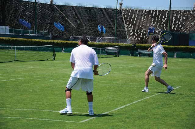
PCME                Test-time        Space           i2t    t2i                              1K Test Images                    5K Test Images
 variant Sampling Similarity Metric complexity        R-P    R-P                              i2t              t2i              i2t             t2i
                                                                         Method
 µ only       7      Mean only           OpN q      24.70 25.64                           PMRP R@1 PMRP R@1 PMRP R@1 PMRP R@1

                                                                         VSE++ [10]         -       64.6     -       52.0     -       41.3     -      30.3
              7      Mean only           OpN q      26.14   26.67
                                                                         PVSE K=1 [47]    40.3˚     66.7   41.8˚     53.5   29.3˚     41.7   30.1˚    30.6
              7      ELK                Op2N q      25.33   25.87        PVSE K=2 [47]    42.8˚     69.2   43.6˚     55.2   31.8˚     45.2   32.0˚    32.4
              7      JS-divergence      Op2N q      25.06   25.55        VSRN [27]        41.2˚     76.2   42.4˚     62.8   29.7˚     53.0   29.9˚    40.5
 PCME
              7      2-Wasserstein      Op2N q      26.16   26.69        VSRN + AOQ [5]   44.7˚     77.5   45.6˚     63.5   33.0˚     55.1   33.5˚    41.1
              3      Average L2         OpJ 2 N q   26.11   26.64
                                                                         PCMEµ only       45.0* 68.0 45.9* 54.6 34.0* 43.5 34.3* 31.7
              3      Match prob         OpJ 2 N q   26.28   26.77        PCME             45.0* 68.8 46.0* 54.6 34.1* 44.2 34.4* 31.9

Table 1. Pairwise distances for distributions. There are many op-       Table 3. Comparison on MS-COCO. PMRP stands for the Plau-
tions for computing the distance between two distributions. What        sible Match R-Precision and R@1 for Recall@1. “˚” denotes re-
are the space complexity and retrieval performances for each op-        sults produced by the published models.
tion? R-P stands for the R-Precision.

                             Image-to-text     Text-to-image            that captures the model performances more accurately than
 Method            HNM
                             R-P     R@1       R-P       R@1            the widely-used R@k metrics. Table 3 shows the results
 VSE0                7       22.4     44.2     22.6         32.7        with state-of-the-art COCO retrieval methods. We observe
 PVSE K=1            3       22.3     40.9     20.5         31.7
                                                                        that the stochastic version of PCME performs better than the
 PVSE K=2            3       19.7     47.3     21.2         28.0        deterministic variant (µ only) across the board. In terms of
 PVSE K=4            3       18.4     47.8     19.9         34.4        the R@1 metric, PVSE K=2 [47], VSRN [27] and AOQ [5]
                                                                        work better than PCME (e.g. 45.2%, 53.0%, 55.1% versus
 PCME µ only         7       24.7     46.4     25.6         35.5
                                                                        44.2% for the 5K, i2t task). However, on the more accu-
 PCME                7       26.3     46.9     26.8         35.2
                                                                        rate PMRP metric, PCME outperforms previous methods
Table 2. Comparison on CUB Caption test split. R-P and R@1              with some margin (e.g. 31.8%, 29.7%, 33.0% versus 34.1%
stand for R-Precision and Recall@1, respectively. The usage of          for the 5K, i2t task). The results on two metric imply that
hardest negative mining (HNM) is indicated.                             PCME retrieves the plausible matches much better than pre-
                                                                        vious methods do. The full results can be found in §E.
an important ingredient for PVSE, we consider the use of                4.4. Understanding the learned uncertainty
the hardest negative mining (HNM). We first observe that
                                                                            Having verified the retrieval performance of PCME, we
PVSE with HNM tends to obtain better performances than
                                                                        now study the benefits of using probabilistic distributions
VSE0 under the R@1 metric, with 47.8% for K=4, com-
                                                                        for representing data. We show that the learned embeddings
pared to 44.2% for VSE0. However, under the R-Precision
                                                                        not only represent the inherent uncertainty of data, but also
metric, we all PVSE models with HNM are worse than
                                                                        enable set algebras among samples that roughly correspond
VSE0 (R-Precision drops from 22.4% for VSE0 to 18.4%
                                                                        to their semantic meanings.
for PVSE K=4). It seems that PVSE with HNM tends to
                                                                        Measuring uncertainty with σ. In an automated decision
retrieve items based on diversity, rather than precision. We
                                                                        process, it benefits a lot to be able to represent uncertainty.
conjecture that the HNM is designed to optimize the R@1
                                                                        For example, the algorithm may refrain from making a de-
performances; more details in §E.2. Comparing PVSE with
                                                                        cision based on the uncertainty estimates. We show that
different values of K, we note that increasing K does not al-
                                                                        the learned cross-modal embeddings capture the inherent
ways bring about performance gains under the R-Precision
                                                                        uncertainty in the instance. We measure the instance-wise
metric (20.5%, 21.2% and 19.9% for K=1,2,4, respectively,
                                                                        uncertainty for all query instances by taking the geometric
for t2i), while the improvement is more pronounced under
                                                                        mean of over the σ P RD entries (§3.2.1). We then com-
the R@1 metric. Finally, PCME provides the best perfor-
                                                                        pute the average R@1 performances in each of the 10 un-
mances on both R-Precision and R@1 metrics, except for
                                                                        certainty bins. Figure 6 plots the correlation between the
the R@1 score for i2t. PCME also improves upon its deter-
                                                                        uncertainty and R@1 on COCO test set. We observe per-
ministic version, PCME µ-only, with some margin: +1.6 pp
                                                                        formance drops with increasing uncertainty. In §F.2, we
and +1.2 pp on i2t and t2i R-Precision scores, respectively.
                                                                        visualize which word affects more to uncertainty. Example
4.3. Results on COCO                                                    uncertain instances and their retrieval results are in §F.3.
                                                                        2D visualization of PCME. To visually analyze the behav-
   As we have identified potential problems with measuring              ior of PCME, we conduct a 2D toy experiment by using
performance on COCO (§4.1.2), we report the results with                9 classes of the CUB Captions (details in §C.3). Figure 5
our Plausible-Match R-Precision (PMRP) metrics (§4.1.1)                 visualizes the learned image and caption embeddings. We

                                                                    7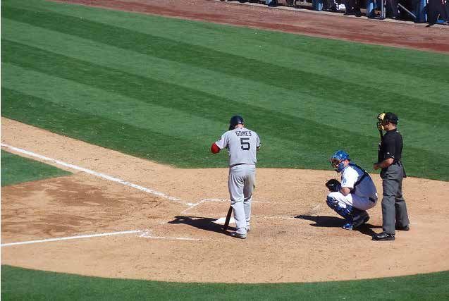
a medium sized bird with a long neck with a white a beautiful small bird with a sharp beak is red
throat, it has a medium sized narrow pointy bill, and red eyes. all over except its back, wings and tail that are brown.
this bird is white with black
and has a long, pointy beak.
this little fellow has a white belly
and breast with stripes of black
on its crown and superciliary.
a larger bird with a bright red head and a colorful black bird with white side and black wings
black and white body, and a long, straight bill. with beige wing bars. bright orange spot on it's side.
99% confidence interval for a beautiful small bird with a sharp beak is red
this bird has . all over except its back, wings and tail that are brown.
Figure 5. Visualization of the probabilistic embedding. The learned image (left) and caption (right) embeddings on 9 subclass of CUB
Captions. Classes are color-coded. Each ellipse shows the 50% confidence region for each embedding. The red ellipse corresponds to the
generic CUB caption, “this bird has ăunką ¨ ¨ ¨ ăunką” with 99% confidence region.
Pied billed Grebe
COCO 1k image sigma vs. Recall@1 COCO 1k caption sigma vs. Recall@1 σx σy = 3.48
σx σy = 3.51
80
58
σx σy = 2.15
70
56
Recall@1
Recall@1
60 54
Red bellied
Woodpecker
σx σy = 0.75
50 52
image-to-text Recall@1 text-to-image Recall@1 Original embedding
0 1 2 3 4 5 6 7 8 9 0 1 2 3 4 5 6 7 8 9 Transformed embedding
Uncertainty bins Uncertainty bins
σx σy Uncetainty level of
each embedding
σx σy = 1.02
Figure 6. σ versus performance. Performance of PCME at dif-
σx σy = 0.76
ferent per-query uncertainty levels in COCO 1k test set. (a) Intersection (mixed) (b) Inclusion (occluded)
Figure 8. Set algebras. For two images, we visualize the em-
CUB 2D image occlusion vs. uncertainty CUB 2D text masking vs. uncertainty beddings for either erased or mixed samples. Mixing (left) and
0.36 0.8
erasing (right) operations roughly translate to the intersection and
0.38 0.6
inclusion relations between the corresponding embeddings.
Average log
Average log
0.40
0.4
0.42
0.2
0.44
0.0
0.46 Image uncertainty Text uncertainty ing an inclusion relationship. We quantitatively verify that
0 22 44 67 89 112134156 179201 0 5 10 15
Occlusion hole size Number of removal tokens the sigma values positively correlate with the ratio of erased
pixels in Figure 7. In COCO, we observe a similar behavior
Figure 7. σ captures ambiguity. Average σ values at different
ratios of erased pixels (for images) and words (for captions).
(shown in §F.1). We discover another positive correlation
between the caption ambiguity induced by erasing words
and the embedding uncertainty.
also plot the embedding for the most generic caption for the
CUB Captions dataset, “this bird has ăunką ăunką . . . ”, 5. Conclusion
where ăunką is a special token denoting the absence of a
word. This generic caption covers most of caption varia- We introduce Probabilistic Cross-Modal Embedding
tions in the embedding space (red ellipses). (PCME) that learns probabilistic representations of multi-
Set algebras. To understand the relationship among distri- modal data in the embedding space. The probabilis-
butions on the embedding space, we artificially introduce tic framework provides a powerful tool to model the
different types of uncertainties on the image data. In Fig- widespread one-to-many associations in the image-caption
ure 8, we start from two bird images and perform erasing pairs. To our knowledge, this is the first work that uses
and mixing transformations [59]. On the embedding space, probabilistic embeddings for a multi-modal task. We exten-
we find that the mixing operation on the images results in sively ablate our PCME and show that not only it improves
embeddings that cover the intersection of the original em- the retrieval performance over its deterministic counterpart,
beddings. Occluding a small region in input images, on the but also provides uncertainty estimates that render the em-
other hand, amounts to slightly wider distributions, indicat- beddings more interpretable.
8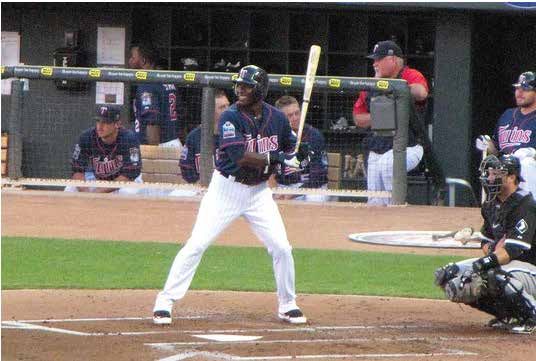
Acknowledgement                                                             [14] David R Hardoon, Sandor Szedmak, and John Shawe-Taylor.
                                                                                 Canonical correlation analysis: An overview with applica-
   We thank our NAVER AI LAB colleagues for valuable                             tion to learning methods. Neural computation, 16(12):2639–
discussions. All experiments were conducted on NAVER                             2664, 2004. 2
Smart Machine Learning (NSML) [21] platform.                                [15] Kaiming He, Xiangyu Zhang, Shaoqing Ren, and Jian Sun.
                                                                                 Deep residual learning for image recognition. In Proc.
References                                                                       CVPR, 2016. 3, 5, 12
                                                                            [16] Byeongho Heo, Sanghyuk Chun, Seong Joon Oh, Dongy-
 [1] Jimmy Lei Ba, Jamie Ryan Kiros, and Geoffrey E Hin-                         oon Han, Sangdoo Yun, Youngjung Uh, and Jung-Woo Ha.
     ton. Layer normalization. arXiv preprint arXiv:1607.06450,                  Slowing down the weight norm increase in momentum-based
     2016. 3, 4                                                                  optimizers. arXiv preprint arXiv:2006.08217, 2020. 5, 12
 [2] Anil Bhattacharyya. On a measure of divergence between                 [17] Yan Huang, Wei Wang, and Liang Wang. Instance-aware im-
     two statistical populations defined by their probability distri-            age and sentence matching with selective multimodal lstm.
     butions. Bull. Calcutta Math. Soc., 35:99–109, 1943. 11                     In Proceedings of the IEEE Conference on Computer Vision
 [3] Samuel R. Bowman, Luke Vilnis, Oriol Vinyals, Andrew                        and Pattern Recognition, pages 2310–2318, 2017. 2
     Dai, Rafal Jozefowicz, and Samy Bengio. Generating sen-                [18] Tony Jebara, Risi Kondor, and Andrew Howard. Probabil-
     tences from a continuous space. In Proceedings of The 20th                  ity product kernels. Journal of Machine Learning Research,
     SIGNLL Conference on Computational Natural Language                         5(Jul):819–844, 2004. 11
     Learning, pages 10–21, Berlin, Germany, Aug. 2016. As-                 [19] Andrej Karpathy and Li Fei-Fei. Deep visual-semantic align-
     sociation for Computational Linguistics. 5, 12                              ments for generating image descriptions. In Proc. CVPR,
 [4] Jie Chang, Zhonghao Lan, Changmao Cheng, and Yichen                         pages 3128–3137, 2015. 6, 12
     Wei. Data uncertainty learning in face recognition. In Proc.           [20] Andrej Karpathy, Armand Joulin, and Li F Fei-Fei. Deep
     CVPR, pages 5710–5719, 2020. 2                                              fragment embeddings for bidirectional image sentence map-
 [5] Tianlang Chen, Jiajun Deng, and Jiebo Luo. Adaptive offline                 ping. In Proc. NeurIPS, pages 1889–1897, 2014. 2
     quintuplet loss for image-text matching. In Proc. ECCV,                [21] Hanjoo Kim, Minkyu Kim, Dongjoo Seo, Jinwoong Kim,
     2020. 7, 15, 16                                                             Heungseok Park, Soeun Park, Hyunwoo Jo, KyungHyun
 [6] Xinlei Chen, Hao Fang, Tsung-Yi Lin, Ramakrishna Vedan-                     Kim, Youngil Yang, Youngkwan Kim, et al. NSML: Meet the
     tam, Saurabh Gupta, Piotr Dollár, and C Lawrence Zitnick.                  MLaaS platform with a real-world case study. arXiv preprint
     Microsoft coco captions: Data collection and evaluation                     arXiv:1810.09957, 2018. 9
     server. arXiv preprint arXiv:1504.00325, 2015. 1, 2, 6                 [22] Diederik P Kingma and Max Welling. Auto-encoding varia-
                                                                                 tional bayes. arXiv preprint arXiv:1312.6114, 2013. 3
 [7] Kyunghyun Cho, Bart Van Merriënboer, Dzmitry Bahdanau,
                                                                            [23] Diederik P. Kingma and Max Welling. Auto-Encoding Vari-
     and Yoshua Bengio. On the properties of neural machine
                                                                                 ational Bayes. In Proc. ICLR, 2014. 2
     translation: Encoder-decoder approaches. arXiv preprint
     arXiv:1409.1259, 2014. 3                                               [24] Thomas N Kipf and Max Welling. Semi-supervised classi-
                                                                                 fication with graph convolutional networks. arXiv preprint
 [8] Terrance DeVries and Graham W Taylor. Improved regular-
                                                                                 arXiv:1609.02907, 2016. 2
     ization of convolutional neural networks with cutout. arXiv
                                                                            [25] Benjamin Klein, Guy Lev, Gil Sadeh, and Lior Wolf. Fisher
     preprint arXiv:1708.04552, 2017. 5, 12
                                                                                 vectors derived from hybrid gaussian-laplacian mixture mod-
 [9] Martin Engilberge, Louis Chevallier, Patrick Pérez, and                    els for image annotation. arXiv preprint arXiv:1411.7399,
     Matthieu Cord. Finding beans in burgers: Deep semantic-                     2014. 2
     visual embedding with localization. In Proc. CVPR, 2018.               [26] Kuang-Huei Lee, Xi Chen, Gang Hua, Houdong Hu, and Xi-
     2, 6, 12                                                                    aodong He. Stacked cross attention for image-text matching.
[10] Fartash Faghri, David J Fleet, Jamie Ryan Kiros, and Sanja                  In Proc. ECCV, 2018. 2, 5
     Fidler. VSE++: Improving visual-semantic embeddings with               [27] Kunpeng Li, Yulun Zhang, Kai Li, Yuanyuan Li, and Yun
     hard negatives. In Proc. BMVC, 2018. 1, 2, 3, 6, 7, 12, 15,                 Fu. Visual semantic reasoning for image-text matching. In
     16                                                                          Proc. ICCV, pages 4654–4662, 2019. 1, 2, 7, 15, 16
[11] Andrea Frome, Greg S Corrado, Jon Shlens, Samy Bengio,                 [28] Xiang Li, Luke Vilnis, Dongxu Zhang, Michael Boratko, and
     Jeff Dean, Marc’Aurelio Ranzato, and Tomas Mikolov. De-                     Andrew McCallum. Smoothing the geometry of probabilistic
     vise: A deep visual-semantic embedding model. In Proc.                      box embeddings. In Proc. ICLR, 2019. 2
     NeurIPS, pages 2121–2129, 2013. 2, 3                                   [29] Tsung-Yi Lin, Michael Maire, Serge Belongie, James Hays,
[12] Yunchao Gong, Liwei Wang, Micah Hodosh, Julia Hocken-                       Pietro Perona, Deva Ramanan, Piotr Dollár, and C Lawrence
     maier, and Svetlana Lazebnik. Improving image-sentence                      Zitnick. Microsoft coco: Common objects in context. In
     embeddings using large weakly annotated photo collections.                  Proc. ECCV, 2014. 6
     In European Conference on Computer Vision, pages 529–                  [30] Chunxiao Liu, Zhendong Mao, An-An Liu, Tianzhu Zhang,
     545. Springer, 2014. 2                                                      Bin Wang, and Yongdong Zhang. Focus your attention: A
[13] Raia Hadsell, Sumit Chopra, and Yann LeCun. Dimension-                      bidirectional focal attention network for image-text match-
     ality reduction by learning an invariant mapping. In Proc.                  ing. In Proceedings of the 27th ACM International Confer-
     CVPR, 2006. 3                                                               ence on Multimedia, page 3–11, 2019. 2, 5

                                                                        9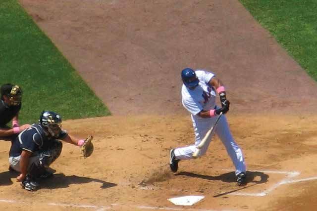
[31] Ilya Loshchilov and Frank Hutter.           Sgdr: Stochas-           [48] Jennifer J Sun, Jiaping Zhao, Liang-Chieh Chen, Florian
     tic gradient descent with warm restarts. arXiv preprint                   Schroff, Hartwig Adam, and Ting Liu. View-invariant prob-
     arXiv:1608.03983, 2016. 5, 12                                             abilistic embedding for human pose. In Proc. ECCV, 2020.
[32] Jiasen Lu, Dhruv Batra, Devi Parikh, and Stefan Lee. Vilbert:             2
     Pretraining task-agnostic visiolinguistic representations for        [49] Christopher Thomas and Adriana Kovashka. Preserving se-
     vision-and-language tasks. In Proc. NeurIPS, pages 13–23,                 mantic neighborhoods for robust cross-modal retrieval. In
     2019. 2, 5                                                                Proc. ECCV, 2020. 2
[33] Jiasen Lu, Vedanuj Goswami, Marcus Rohrbach, Devi                    [50] Ashish Vaswani, Noam Shazeer, Niki Parmar, Jakob Uszko-
     Parikh, and Stefan Lee. 12-in-1: Multi-task vision and                    reit, Llion Jones, Aidan N Gomez, Łukasz Kaiser, and Illia
     language representation learning. In Proceedings of the                   Polosukhin. Attention is all you need. In Advances in neural
     IEEE/CVF Conference on Computer Vision and Pattern                        information processing systems, pages 5998–6008, 2017. 4
     Recognition, pages 10437–10446, 2020. 2, 5                           [51] Luke Vilnis and Andrew McCallum. Word representations
[34] Kevin P Murphy. Machine learning: a probabilistic perspec-                via gaussian embedding. In Proc. ICLR, 2015. 2
     tive. MIT press, 2012. 2                                             [52] Liwei Wang, Yin Li, and Svetlana Lazebnik. Learning deep
[35] Kevin Musgrave, Serge Belongie, and Ser-Nam Lim. A met-                   structure-preserving image-text embeddings. In Proc. CVPR,
     ric learning reality check. In Proc. ECCV, 2020. 6, 13                    pages 5005–5013, 2016. 1, 2
[36] Hyeonseob Nam, Jung-Woo Ha, and Jeonghee Kim. Dual                   [53] Tongzhou Wang and Phillip Isola. Understanding contrastive
     attention networks for multimodal reasoning and matching.                 representation learning through alignment and uniformity on
     In Proceedings of the IEEE Conference on Computer Vision                  the hypersphere. In International Conference on Machine
     and Pattern Recognition, pages 299–307, 2017. 2, 5                        Learning, 2020. 4, 11
[37] Arvind Neelakantan, Jeevan Shankar, Alexandre Passos, and            [54] Zihao Wang, Xihui Liu, Hongsheng Li, Lu Sheng, Junjie
     Andrew McCallum. Efficient non-parametric estimation of                   Yan, Xiaogang Wang, and Jing Shao. CAMP: Cross-modal
     multiple embeddings per word in vector space. In Proc.                    adaptive message passing for text-image retrieval. In Proc.
     EMNLP, pages 1059–1069, 2014. 2                                           ICCV, 2019. 2, 5
[38] Dat Quoc Nguyen, Ashutosh Modi, Stefan Thater, Manfred
                                                                          [55] Xi Wei, Tianzhu Zhang, Yan Li, Yongdong Zhang, and Feng
     Pinkal, et al. A mixture model for learning multi-sense word
                                                                               Wu. Multi-modality cross attention network for image and
     embeddings. In Proceedings of the 6th Joint Conference on
                                                                               sentence matching. In Proc. CVPR, 2020. 2, 5
     Lexical and Computational Semantics (* SEM 2017), pages
                                                                          [56] P. Welinder, S. Branson, T. Mita, C. Wah, F. Schroff, S. Be-
     121–127, 2017. 2
                                                                               longie, and P. Perona. Caltech-UCSD Birds 200. Technical
[39] Seong Joon Oh, Kevin Murphy, Jiyan Pan, Joseph Roth, Flo-
                                                                               Report CNS-TR-2010-001, California Institute of Technol-
     rian Schroff, and Andrew Gallagher. Modeling uncertainty
                                                                               ogy, 2010. 2, 6
     with hedged instance embedding. In Proc. ICLR, 2019. 2, 3,
     4                                                                    [57] Yongqin Xian, Bernt Schiele, and Zeynep Akata. Zero-shot
[40] Jeffrey Pennington, Richard Socher, and Christopher D Man-                learning-the good, the bad and the ugly. In Proceedings of the
     ning. Glove: Global vectors for word representation. In Proc.             IEEE Conference on Computer Vision and Pattern Recogni-
     EMNLP, 2014. 3, 5, 12                                                     tion, pages 4582–4591, 2017. 6
[41] Scott Reed, Zeynep Akata, Honglak Lee, and Bernt Schiele.            [58] Peter Young, Alice Lai, Micah Hodosh, and Julia Hocken-
     Learning deep representations of fine-grained visual descrip-             maier. From image descriptions to visual denotations: New
     tions. In Proc. CVPR, pages 49–58, 2016. 6                                similarity metrics for semantic inference over event descrip-
[42] Shaoqing Ren, Kaiming He, Ross Girshick, and Jian Sun.                    tions. ACL, 2:67–78, 2014. 1
     Faster r-cnn: Towards real-time object detection with region         [59] Sangdoo Yun, Dongyoon Han, Seong Joon Oh, Sanghyuk
     proposal networks. In Proc. NeurIPS, pages 91–99, 2015. 2                 Chun, Junsuk Choe, and Youngjoon Yoo. Cutmix: Regu-
[43] Edgar Schonfeld, Sayna Ebrahimi, Samarth Sinha, Trevor                    larization strategy to train strong classifiers with localizable
     Darrell, and Zeynep Akata. Generalized zero-and few-                      features. In Proc. ICCV, 2019. 8
     shot learning via aligned variational autoencoders. In Proc.         [60] Qi Zhang, Zhen Lei, Zhaoxiang Zhang, and Stan Z. Li.
     CVPR, pages 8247–8255, 2019. 2                                            Context-aware attention network for image-text retrieval. In
[44] Tyler Scott, Karl Ridgeway, and Michael Mozer. Stochastic                 Proc. CVPR, 2020. 2, 5
     prototype embeddings. ICML Workshop on Uncertainty and
     Robustness in Deep Learning, 2019. 2
[45] Yichun Shi and Anil K Jain. Probabilistic face embeddings.
     In ICCV, 2019. 2
[46] Anna Silnova, Niko Brummer, Johan Rohdin, Themos Stafy-
     lakis, and Lukas Burget. Probabilistic embeddings for
     speaker diarization. In Proc. Odyssey 2020 The Speaker and
     Language Recognition Workshop, pages 24–31, 2020. 2
[47] Yale Song and Mohammad Soleymani. Polysemous visual-
     semantic embedding for cross-modal retrieval. In Proc.
     CVPR, pages 1979–1988, 2019. 2, 3, 4, 5, 6, 7, 11, 15, 16

                                                                     10
Supplementary Materials Kullback–Leibler (KL) divergence measures the dif-
ference between two distributions as follows:
We include additional materials in this document. We ż
describe additional details on PCME to complement the p
KLpp, qq “ log dp
main paper (§A). Various probabilistic distances are intro- q
(B.1)
σ22 σ12 pµ1 ´ µ2 q2
„
duced (§B). We provide the experimental protocol details 1
(§C), ablation studies (§D), and additional results (§E). Fi- “ log 2 ` 2 ` .
2 σ1 σ2 σ22
nally, more uncertainty analyses are shown (§F).
KL divergence is not a metric because it is asymmetric
A. More details for PCME (KLpp, qq ‰ KLpq, pq) and does not satisfy the triangu-
lar inequality. If q has very small variance, nearly zero,
In this section, we provide details for PCME. the KL divergence between p and q will be explored. In
A.1. The uniformity loss other words, if we have a very certain embedding, which
has nearly zero variance, in our gallery set, then the cer-
Recently, Wang et al. [53] propose the uniformity loss tain embedding will be hardly retrieved by KL divergence
which enforces the feature vectors to distribute uniformly measure. In the latter section, we will show that KL diver-
on the unit hypersphere. In Wang et al. [53], the uniformity gence leads to bad retrieval performances in the real-world
loss was shown to lead to better representations for L2 nor- scenario.
malized features. Since our µ vectors are projected to the Jensen-Shannon (JS) divergence is the average of for-
unit L2 hypersphere, we also employ the uniformity loss to ward (KLpp, qq) and reverse (KLpq, pq) KL divergences.
learn better representations. We apply the uniformity loss Unlike KL divergence, the square root of JS divergence is a
J J
on the joint embeddings Z “ tv11 , t11 , . . . , vB , tB u in the metric function.
mini-batch size of B as follows:
1
ÿ 1 2 JSpp, qq “ rKLpp, qq ` KLpq, pqs . (B.2)
LUnif “ e´2}z´z }2 . (A.1) 2
z,z 1 PZˆZ Like KL divergence, JS divergence still has division term
A.2. Connection of soft contrastive loss to the MIL by variances σ1 , σ2 , it can be numerically unstable when
objective of PVSE the variances are very small.
Probability product kernels [18] are generalized inner
In the main text we presented an analysis based on gradi- product for two distributions, that is:
ents to study how the loss function in Equation (1) handles ż
plurality in cross-modal matches and learns uncertainties in P P Kpp, qq “ ppzqρ qpzqρ dz. (B.3)
data. Here we make connections with the MIL loss used by
PVSE (§3.1.1, [47]); this section follows the corresponding When ρ “ 1, it is called the expected likelihood kernel
section in the main paper. (ELK), and when ρ “ 1{2, it is called Bhattacharyya’s
To build connections with PVSE, consider a one-hot affinity [2], or Bhattacharyya kernel.
weight array wjj 1 where, given that pv, tq is a positive pair, Expected likelihood kernel (ELK) is a special case of
the “one” value is taken only by the single pair pj, j 1 q whose PPK when ρ “ 1 in Equation (B.3). In practice, we take log
distance is smallest. Define wjj 1 for a negative pair pv, tq to compute ELK as follows:
conversely. Then, we recover the MIL loss used in PVSE,
1 pµ1 ´ µ2 q2
„
where only the best match among J 2 predictions are uti- 2 2
ELKpp, qq “ ` logpσ 1 ` σ2 q . (B.4)
lized. As we see in the experiments, our softmax weight 2 σ12 ` σ22
scheme provides a more interpretable and performant su-
pervision for the uncertainty than the argmax version used Bhattacharyya kernel (BK) is another special case of
by PVSE. PPK when ρ “ 1{2 in Equation (B.3). The log BK is de-
fined as the follows:
B. Probabilistic distances 1 pµ1 ´ µ2 q2
„
σ2 σ1
BKpp, qq “ ` 2 logp ` q . (B.5)
We introduce probabilistic distance variants to mea- 4 σ12 ` σ22 σ1 σ2
sure the distance between two normal distributions p “ Wasserstein distance is a metric function of two dis-
N pµ1 , σ12 q and q “ N pµ2 , σ22 q. All distance functions are tributions on a given metric space M . The Wasser-
non-negative, and become zero if and only if two distribu- stein distance between two normal distributions on R1 , 2-
tions are identical. Extension to multivariate Gaussian dis- Wasserstein distance, is defined as follows:
tributions with diagonal variance can be simply derived by
taking the summation over the dimension-wise distances. W pp, qq2 “ pµ1 ´ µ2 q2 ` σ1 ´ σ2 2 . (B.6)
11Number of categories in MS-COCO validation images in an end-to-end fashion. We use the ResNet-152 backbone
30 with embedding dimension D “ 1024 for MS-COCO and
ResNet-50 with D “ 512 for CUB. For all experiments, we
25 set the number of samples J “ 7 (the detailed study is in
Number of images
20 §E). We use AdamP optimizer [16] with the cosine learning
rate scheduler [31] for a stable training.
15
10 MS-COCO. We follow the evaluation protocol of [19]
where the validation set is added to the training pool (re-
5
ferred to as rV in [9, 10]). Our training and validation splits
0 contain 113,287 and 5,000 images, respectively. We report
1 2 3 4 5 6 7 8 9 10 results on both 5K and (the average over 5-fold) 1K test sets.
Number of distinct categories per image
Figure C.1. Number of distinct categories in MS-COCO valida- Hyperparameter search protocol. We validate the initial
tion set. Images which have more than 10 categories are omitted. learning rate, number of epochs for the warm-up and fine-
tuning, and other hyperparameters on the 150 CUB training
C. Experimental Protocol Details classes and the MS-COCO caption validation split. For MS-
COCO, we use the initial learning rate as 0.0002, 30 warm-
We introduce the cross-modal retrieval benchmarks con- up and 30 finetune epochs. Weights for regularizers LKL
sidered in this work. We discuss the issues with the current and LUnif are set to 0.00001 and 0, respectively. For CUB
practice for evaluation and introduce new alternatives. Caption, the initial learning rate is 0.0001, the number of
warm-up epochs 10 and fine-tuning epochs 50. Weights for
C.1. Plausible Match R-Precision (PMRP) details
regularizers LKL and LUnif are set to 0.001 and 10, respec-
In this work, we seek more reliable sources of pairwise tively. For both datasets, models are always trained with
similarity measurements through class and attribute labels Cutout [8] and random caption dropping [3] augmentation
on images. For example, on CUB caption dataset, we have strategies with 0.2 and 0.1 erasing ratios, respectively. The
established the positivity of pairs by the criterion that a pair initial values for a, b in Equation (3) are set to -15 and 15
pi, cq is positive if and only if both elements in the pair be- for COCO (-5 and 5 for CUB), respectively.
long to the same bird class. Similarly, on COCO caption
dataset, we judge the positivity through the multiple class C.3. CUB 2D toy experiment details
labels (80 classes total) attached per image: a pair pi, cq We select nine bird classes from CUB caption; three
is positive if and only if the binary class vectors for the swimming birds (“Western Grebe”, “Pied Billed Grebe”,
two instances, y i , y c P t0, 1u80 , differ at most at ζ posi- “Pacific Loon”), three small birds (“Vermilion Flycatcher”,
tions (Hamming Distance). Note that because we use R- “Black And White Warbler”, “American Redstart”), and
Precision, the ratio of positive items in top-r retrieved items three woodpeckers (“Red Headed Woodpecker”, “Red Bel-
where r is the number of the ground-truth matches, increas- lied Woodpecker”, “Downy Woodpecker”).
ing ζ will make r larger, and will penalize methods more, We slightly modify PCME to learn 2-dimensional em-
which retrieve irrelevant items. beddings. For the image encoder, we use the same structure
In Figure C.1, we visualize the number of distinct cate- as the other experiments, but omitting the attention modules
gories per image in MS-COCO validation set. In the figure, from the µ and σ modules. For the caption encoder, we train
we can observe that about the half of images have more 1024-dimensional bi-GRU on top of GloVe vectors, and ap-
than two categories. To avoid penalty caused by almost ne- ply two 2D projections to get the 1024 dimensional µ and
glectable objects (as shown in Figure C.2), we set ζ “ 2 for σ embedding. The other training details are the same as the
measuring PMRP score. For PMRP with different ζ rather other CUB caption experiments.
than 2, results can be found in §E.
C.2. Implementation details D. Ablation studies
Common. As in Faghri et al. [10], we use the ImageNet- We provide ablation studies on PCME for regularization
pretrained ResNet [15] and the pretrained GloVe with 2.2M terms, σ module architectures, number of samples J during
vocabulary [40] for initializing the visual and textual en- training, and embedding dimension D.
coders (fV , fT ). We first warm-up the models by training
the head modules for each modality, with frozen feature ex- Regularizing uncertainty. PCME predicts probabilistic
tractors. Afterwards, the whole parameters are fine-tuned outputs. We have considered uncertainty-specific regular-
12You can also read