The Shape of Art History in the Eyes of the Machine
←
→
Page content transcription
If your browser does not render page correctly, please read the page content below
The Shape of Art History in the Eyes of the Machine∗
                                           Ahmed Elgammal1†            Marian Mazzone2         Bingchen Liu1     Diana Kim1
                                                                           Mohamed Elhoseiny1
                                                               The Art and Artificial Intelligence Laboratory
                                                      1
                                                        Department of Computer Science, Rutgers University, NJ, USA
arXiv:1801.07729v2 [cs.AI] 12 Feb 2018

                                                        2
                                                          Department of Art History, College of Charleston, SC, USA

                                                                                               Abstract
                                                      How does the machine classify styles in art? And how does it relate to art historians’ meth-
                                                  ods for analyzing style? Several studies have shown the ability of the machine to learn and
                                                  predict style categories, such as Renaissance, Baroque, Impressionism, etc., from images of
                                                  paintings. This implies that the machine can learn an internal representation encoding discrim-
                                                  inative features through its visual analysis. However, such a representation is not necessarily
                                                  interpretable. We conducted a comprehensive study of several of the state-of-the-art convolu-
                                                  tional neural networks applied to the task of style classification on 77K images of paintings,
                                                  and analyzed the learned representation through correlation analysis with concepts derived
                                                  from art history. Surprisingly, the networks could place the works of art in a smooth temporal
                                                  arrangement mainly based on learning style labels, without any a priori knowledge of time
                                                  of creation, the historical time and context of styles, or relations between styles. The learned
                                                  representations showed that there are few underlying factors that explain the visual variations
                                                  of style in art. Some of these factors were found to correlate with style patterns suggested
                                                  by Heinrich Wölfflin (1846-1945). The learned representations also consistently highlighted
                                                  certain artists as the extreme distinctive representative of their styles, which quantitatively con-
                                                  firms art historian observations.

                                                Keywords: Artificial Intelligence — Computational Art History
                                            ∗
                                               This paper is an extended version of a paper that will be published on the 32nd AAAI conference on Artificial
                                         Intelligence, to be held in New Orleans, USA, February 2-7, 2018
                                             †
                                               Corresponding author: Ahmed Elgammal elgammal@cs.rutgers.edu

                                                                                                   1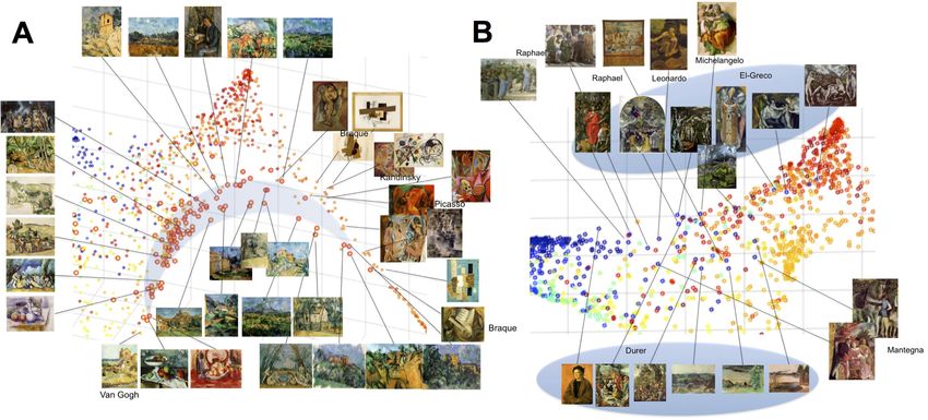
Art history could prove “to contain unexpected potentialities as a predictive science” – George
             Kubler, The Shape of Time: Remarks on the History of Things, 1962.

1    Introduction
Style is central to the discipline of art history. The word “style” is used to refer to the individual
way or manner that someone makes or does something, for example Rembrandt’s style of painting.
Style also refers to groups of works that have a similar typology of characteristics, such as the
Impressionist style, or High Renaissance style. Art historians identify, characterize, and define
styles based on the evidence of the physical work itself, in combination with an analysis of the
cultural and historical features of the time and place in which it was made. Although we see style,
and we all know that it exists, there is still no central, agreed upon theory of how style comes about,
or how and why it changes. Some of the best scholars of art history have written persuasively about
the importance of style to the discipline, and the concomitant difficulty of defining or explaining
what it is and why it changes [1, 2]. Up to now connoisseurship has proven to be one of the
most effective means to detect the styles of various artists, and differentiate style categories and
distinctions in larger movements and periods.
     Recent research in computer vision and machine learning have shown the ability of the ma-
chine to learn to discriminate between different style categories such as Renaissance, Baroque,
Impressionism, Cubism, etc., with reasonable accuracy, (e.g. [3, 4, 5, 6]). However, classifying
style by the machine is not what interests art historians. Instead, the important issues are what
machine learning may tell us about how the characteristics of style are identified, and the patterns
or sequence of style changes. The ability of the machine to classify styles implies that the ma-
chine has learned an internal representation that encodes discriminative features through its visual
analysis of the paintings. However, it is typical that the machine uses visual features that are not
interpretable by humans. This limits the ability to discover knowledge out of these results.
     Our study’s emphasis is on understanding how the machine achieves classification of style,
what internal representation it uses to achieve this task, and how that representation is related to art
history methodologies for identifying styles. To achieve such understanding, we utilized one of the
key formulations of style pattern and style change in art history, the theory of Heinrich Wölfflin
(1846-1945). Wölfflin’s comparative approach to formal analysis has become a standard method of
art history pedagogy. Wölfflin chose to separate form analysis from discussions of subject matter
and expression, focusing on the “visual schema” of the works, and how the “visible world crys-
tallized for the eye in certain forms” [7]. Wölfflin identified pairs of works of art to demonstrate
style differences through comparison and contrast exercises that focused on key principles or fea-
tures. Wölfflin used his method to differentiate the Renaissance from the Baroque style through
five key visual principles: linear/painterly, planar/recessional, closed form/open form, multiplic-
ity/unity, absolute clarity/relative clarity. Wölfflin posited that form change has some pattern of
differentiation, such that style types and changes can only come into being in certain sequences.
     With advances in computer vision and machine learning and the availability of comprehensive
datasets of images, we are now positioned to approach the history of art as a predictive science, and
relate its means of determining questions of style to machine results. Lev Manovich has argued
that the use of computational methods, while providing a radical shift in scale, in fact continues the
humanities’ traditional methodologies [8]. It was nearly impossible to apply and empirically test

                                                   2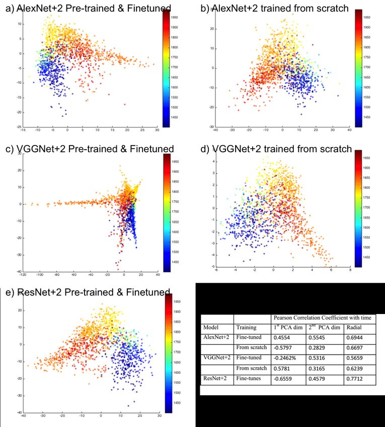
Wölfflin’s methods of style differentiation and analysis before developments in computer science.
No human being would assemble the number of examples needed to prove the value of his methods
for finding discriminative features. Nor could anyone amass the dataset necessary to demonstrate
the usefulness of his model for processing style description and sequencing beyond the immediate
examples of Renaissance and Baroque via his five pairs. We chose Wölfflin’s theory because of his
emphasis on formal, discriminative features and the compare/contrast logic of his system, qualities
that make it conducive to machine learning. Today, art historians use a wide variety of methods that
are not only solely focused on form, but for the type of analysis of this paper Wölfflin’s approach
is useful.

Methodology
Deep convolutional neural networks have recently played a transformative role in advancing arti-
ficial intelligence [9]. We evaluated a large number of state-of-the-art deep convolutional neural
network models, and variants of them, trained to classify styles. We focused on increasing the
interpretability of the learned presentation by forcing the machine to achieve classification with
a reduced number of variables without sacrificing classification accuracy. We then analyzed the
achieved representations through linear and nonlinear dimensionality reduction of the activation
space, visualization, and correlation analysis with time and with Wölfflin’s pairs. We used a col-
lection of 77K digitized paintings to train, validate and test the models. We utilized two sets of
digitized paintings for visualization and correlation analysis of the achieved representations. In
particular, we used variants of AlexNet [10], VGGNet [11], ResNet [12], which were originally
developed for the task of object categorization for the ImageNet challenge [13] and each of them
raised the state of the art in that task when they were introduced. We adapted these networks
for classifying 20 style classes. Our study included varying the training strategies (training from
scratch on art data vs. using pre-trained models and fine-tuning them on art data), varying the
network architecture, and data augmentation strategies.

Main Results
Trained to predict styles, based only on noisy discrete style labels, without being given any notion
of time, the machine encoded art history in a smooth chronology. The learned representation can
be explained based on a handful of factors. The first two modes of variations are aligned with the
concepts of linear vs. painterly and planer vs. recessional suggested by Heinrich Wölfflin (1846-
1945), and quantitatively explain most of the variance in art history, where temporal progression
correlates radially across these modes (See Figure 1). The importance of these results is that they
show that the selected art historian’s theories about style change can be quantifiably verified using
scientific methods. The results also show that style, which appears to be a subjective issue, can be
computationally modeled with objective means.

                                                 3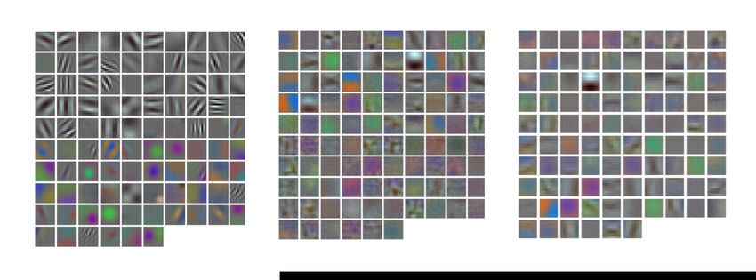
Marc
        A
                                                            Cézanne
                                    Monet       Sisley                Cézanne                               Picasso
              Renoir

                 Sisley
                                                                                                                                                                           Picasso

                                                                                                                                                                            Gris
         Manet

                                                                                                                                                                           Braque
                     Goya

          Rubens
                                                                                                                                                                       Malevich

                    Velázquez

       Rembrandt

                                                                                                                                                                           Warhol
        Rembrandt

                                                                                     Malevich                          Mondrian                          Rothko
                          Raphael    Van Eyck     Raphael       Da Vinci

        B                                                                   C
                                                                                    Wölfflin's)concepts)
                                                                                     Correla'on)with)

                                                                                                                                           2%

                                                                                                                                           1%

                                                                                                         !0.6% !0.5% !0.4% !0.3% !0.2% !0.1%    0%   0.1% 0.2% 0.3% 0.4%

                                                                                                                        1%                                2%
                                                                                Absolute%vs%Rela6ve%
                                                                                                                     0.0015%                            0.198%
                                                                                      Clarity%
                                                                                Mul6plicity%vs%Unity%                !0.0302%                          0.2267%
                                                                                Planer%vs%Recession%                 !0.4946%                          !0.0736%
                                                                                Close%vs%Open%                       0.2448%                           0.1724%
                                                                                Linear%vs%Painterly%                 !0.2336%                          0.3547%

Figure 1: Modes of variations of the activation subspace showing smooth temporal transition and correlation with
Wölfflin’s concepts. (A) First and second modes of variations of the AlexNet+2 model with paintings color-coded
by date of creation. The first mode (the horizontal axis) seems to correlate with figurative art, which was dominant
till Impressionism, vs. non-figurative, distorted figures, and abstract art that dominate 20th century styles. Another
interpretation for this dimension is that it reflects Wölfflin’s concept of plane (to the right) vs. recession (to the left).
This axis correlates the most with Wölfflin’s concept of plane vs. recession with -0.50 PCC. The vertical axis correlates
with the linear (towards the bottom) vs. painterly (towards the top) concept (0.36 PCC). (B) The angular coordinate
exhibits strong correlation with time (PCC of 0.69). (C) Correlation with Wölfflin’s concepts.

                                                                      4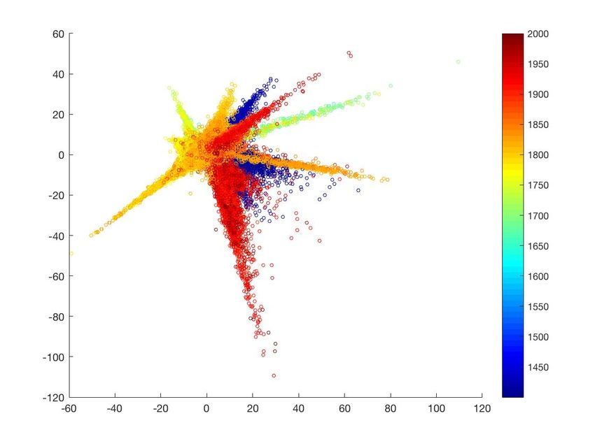
2        Detailed Methodology
2.1        Challenges with Art Style Classification
In contrast to the typical object classification in images, the problem of style classification in art has
a different set of challenges that we highlight here. Style is not necessarily correlated with subject
matter, which corresponds to existence of certain objects in the painting. Style is mainly related
to the form and can be correlated with features at different levels, low, medium and high-level. As
a result, it is not necessary that networks which perform better for extracting semantic concepts,
such as object categories, would be perform as well in style classification. In the literature of object
classification, deeper networks were shown to perform better [11, 12] since they facilitate richer
representations to be learned at different levels of features. We do not know if a deeper network
will necessarily be better in the style classification domain. This remains something to discover
through our empirical study. However, the challenge, in the context of art style classification, is
the lack of images on a scale of magnitude similar to ImageNet (million of images). The largest
publicly available dataset, which we use, is only in the order of 80K images. This limitation is due
to copyright issue, which is integral to the domain of art. Moreover, collecting annotation in this
domain is hard since it requires expert annotators and typical crowd sourcing annotators are not
qualified.
    Another fundamental difference is that styles do no lend themselves to discrete mutually exclu-
sive classes as in supervised machine learning. Style transition over time is typically smooth, and
style labels are after-the-fact concepts imposed by art historians, sometimes centuries later. Paint-
ings can have elements that belongs to multiple styles, and therefore not necessarily identifiable
with a unique style class.
    Paintings also come in wide variety of sizes. The canvas can span a couple of hundreds of
square feet or can be as small as a couple of square inches. The aspect ratio can vary very signif-
icantly as well. A typical CNN requires its input to be resized to a fixed size retinal array. This
bound to introduce geometric distortions, which can affect the composition, and loss of details re-
lated to surface texture carrying essential information about brush strokes. Both composition and
brush strokes are essential to identify style. In this paper we do no address solving these issues.
We mainly report the behavior of the studied model for style classification despite their limitation
to address these issues.

2.2        Datasets
Training-testing Set: We trained, validated, and tested the networks using paintings from the pub-
licly available WikiArt dataset1 . This collection (as downloaded in 2015) has images of 81,449
paintings from 1,119 artists ranging from the fifteenth century to contemporary artists. Several
prior studies on style classification used subsets of this dataset (e.g. [4, 5, 6]). Originally WikiArt
has 27 style classes. For the purpose of our study we reduced the number of classes to 20 classes by
merging fine-grained style classes with small number of images, for example we merged cubism,
analytical cubism, and synthetic cubism into one cubism class. Table 1 shows a list of the 20 style
classes used and their mapping from the original WikiArt classes. We also ignored the symbolism
    1
        Wikiart dataset http://www.wikiart.org

                                                    5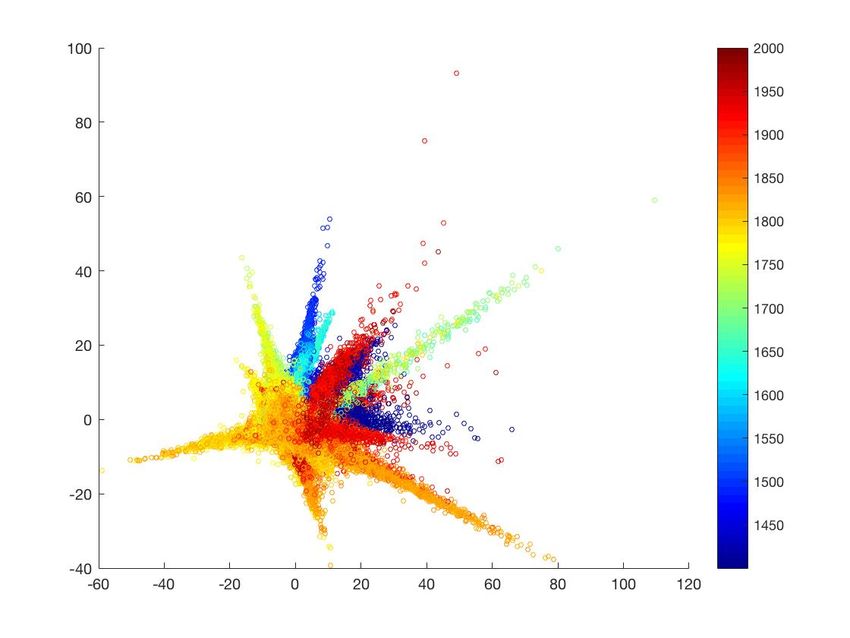
style class since in the Wikiart collection this class contains various paintings from different styles
that erroneously labeled as “symbolism”. In general, by visual inspection we notice that the style
labels in the WikiArt collection is noisy and not accurate. However, it remains the largest pub-
licly available collection. Other available collections, which might be cleaner in their labels, are
typically much smaller in size for the purpose of training a deep network. We excluded from the
collections images of sculptures and photography. The total number of images used for training,
validation, and testing are 76,921 images. We split the data into training (85%), validation (9.5%)
and test sets (5.5%).

                               Table 1: Style classes used in learning the models

                         Style Class            Number of Images                   Merged styles
          1          Early Renaissance               1391
          2          High Renaissance                1343
          3    Mannerism and Late Renaissance        1279
          4        Northern Renaissance              2552
          5               Baroque                    4241
          6                Rococo                    2089
          7             Romanticism                  7019
          8            Impressionism                13060
          9         Post-Impressionism               6965                  Post Impressionism+Pointillism
          10              Realism                   11528          Realism + Contemporary Realism + New Realism
          11            Art Nouveau                  4334
          12               Cubism                    2562          Cubism + Analytical Cubism + Synthetic Cubism
          13           Expressionism                 6736
          14              Fauvism                    934
          15      Abstract-Expressionism             2881             Abstract Expressionism & Action Painting
          16        Color field painting             1615
          17            Minimalism                   1337
          18       Naı̈ve art-Primitivism            2405
          19              Ukiyo-e                    1167
          20               Pop-art                   1483
                  Total number of Images            76921

     Visualization Set I: We used another smaller dataset containing 1485 images of paintings from
the Artchive dataset2 to analyze and visualize the representation. Previous researches that have
used this dataset (e.g. [5]). We denote this dataset in this paper as the “Visualization dataset I”.
While the WikiArt collection is much bigger in size, this dataset contains a better representation
of the important works of western art from 1400-2000AD by 60 artists. Therefore, we mainly use
it to visualize and analyze the learned representation. We excluded from the collections images
of sculptures and images containing partial details of paintings. We also collected art historian’s
rating annotations (scale of 1 to 5) for each of the Wölfflin’s pairs for 1000 paintings from this data
set and use it in our correlation analysis.
     Visualization Set II: We also used 62K painting from the Wikiart dataset for visualization and
analysis of the representations. We only included paintings that have date annotations for the
purposes of visualization and temporal correlation. The two chosen visualization sets have com-
plementary properties. While the Artchive visualization set represents knowledge about influential
and important artists, the Wikiart is more arbitrarily chosen based on what is available in the public
   2
       Artchive dataset http://www.artchive.com

                                                           6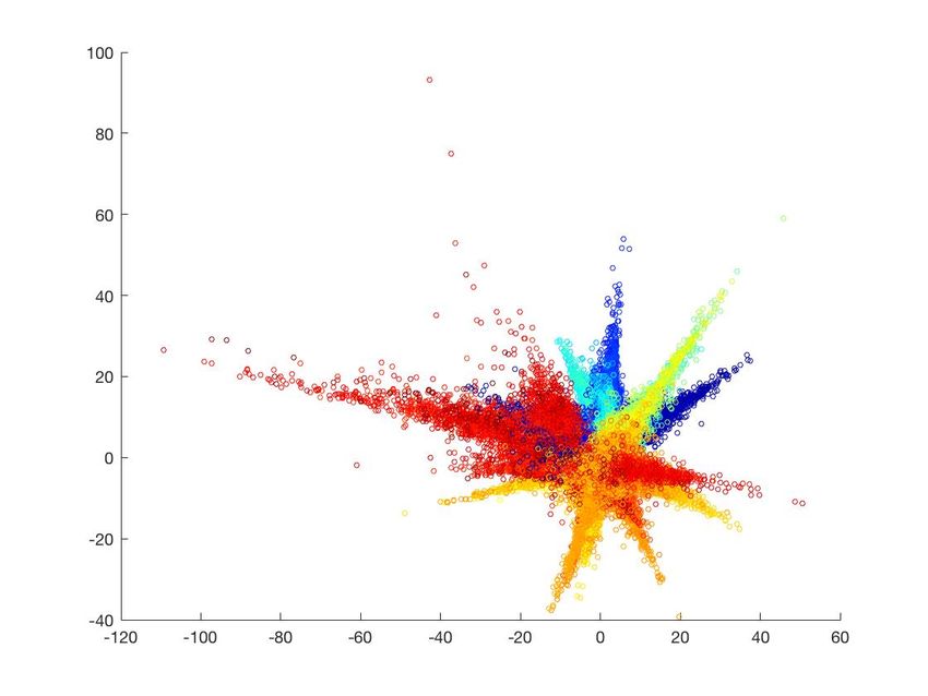
domain. The Artchive dataset lacks paintings from the 18th century and does not have broad sam-
pling of early 19th paintings or post-war 20th century. In contrast, the Wikiart dataset is lacking
certain works of art that art historians would consider important, nevertheless it densely samples a
broad range of styles. In addition, the Wikiart dataset has a large bias towards 20th century art and
post WWII works.

2.3    Studied Deep Learning Models:
We performed a comprehensive comparative study on several deep convolutional networks, adapted
for the task of style classification. For the purpose of this paper, we report the results of three main
networks: AlexNet [10], VGGNet [11], and ResNet [12], as well as variants of them. All these
models were originally developed for the task of object recognition for the ImageNet challenge [13]
and each of them raised the state of the art when they were introduced.
    For the non-expert reader, here we briefly summarize the main features of each of these models.
Deep convolutional networks in general consist of a sequence of layers of artificial neural units
of different types. Convolutional layers apply learned filters (templates) to each location of its
input image. These convolutional layers are interleaved with pooling layers, which aggregate the
responses of the convolution layers. Typically, the sequence of convolution and pooling layers
results in re-representing the visual information in the image as responses to a large number of
learned filters applied to wider and wider regions of the image as the information propagates deeper
in the network. Such filters are learned or tuned by the machine in response to the task in hand.
Finally the responses are passed to a sequence of fully connected layers that acts as a classifier.
    AlexNet [10] architecture consists of five consecutive convolution layers, interleaved with some
pooling layers, followed by three fully connected layers, resulting in 1000 nodes representing the
object classes in ImageNet. The convolutional filters have different sizes at each layer, starting
from big filters (11x11) and reduced the filter size at following layers. In contrast VGGNet [11]
adapted an architecture of fixed size filters (3x3) over a deeper sequence of convolutional layers.
Residual Networks (ResNet [12]) introduced shortcut connection between the convolution layers
outputs and later layers, which results in much deeper architectures, reaching over 150 layers.
    In our study, in general for all the models, the final softmax layer, originally designed for the
1000 classes in ImageNet, was removed and replaced with a layer of 20 softmax nodes, one for
each style class. Two modes of training were evaluated, 1) training the models from scratch on
the Wikiart data set, described above; 2) using a pre-trained model with ImageNet data and fine-
tuned on the Wikiart data. Fine-tuning is the standard practice when adapting well-performing
pre-trained models to a different domain.

2.4    Increasing the interpretability of the representation
Having a large number of nodes at the fully connected layer allows the representation to project the
data into a very high dimensional space where classification would be easy (especially in our case
with only 20 classes), without forcing similar paintings across styles to come closer in the repre-
sentation. To increase the interpretability of the representation, we force the network to achieve
classification through a lower dimension representation. To achieve this, after training the network
(whether from scratch or through fine-tuning), two more fully connected layers were added with
a reduced number of nodes. These reduced dimensional layers force the representation to use a

                                                   7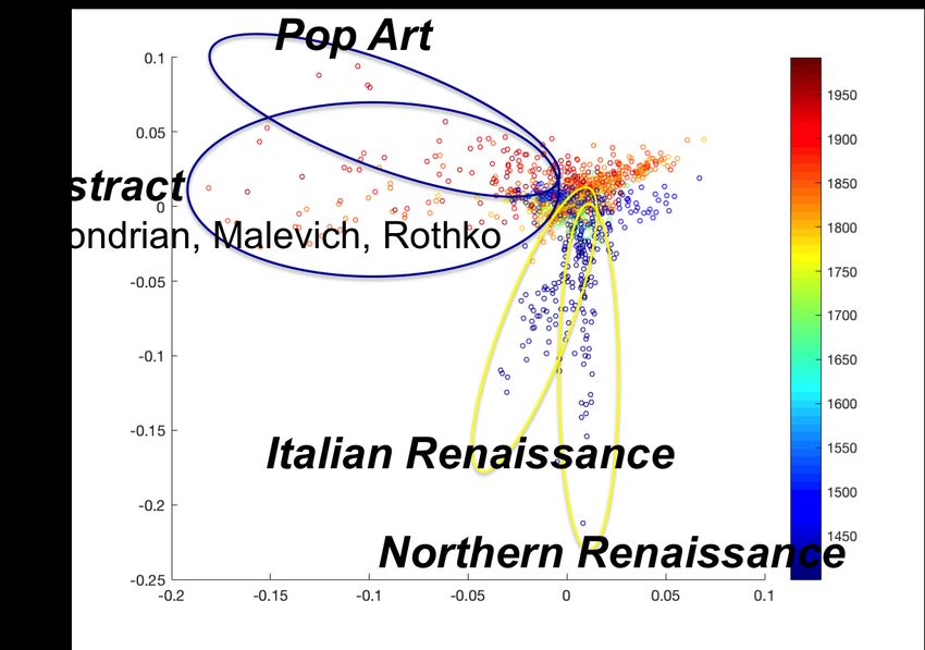
smaller number of degrees of freedom, which in turn forces paintings across styles to come closer
in the representation based on their similarity. In particular, we added two layers with 1024 and
512 nodes to all the models, and the models were then fine-tuned to adjust the weights for the new
layers. As will be shown later, adding these dimensionality reduction layers did not affect the clas-
sification accuracy. The experiments showed that gradually reducing the number of nodes in the
fully connected layers forced the network to achieve a “smoother” and interpretable representation.
It is important to emphasize that to achieve this effect without reducing the accuracy; the two new
layers have to be added after the network is trained, then models are fine-tuned. Training the full
architecture with the two extra layers, whether from scratch of fine-tuned, typically doesn’t result
in converging to similar accuracy.
     We analyzed the modes of variations in the activation of each layer of the learned representa-
tion using Principle component analysis (PCA) [14]. We also analyzed the activation space using
Independent Component Analysis (ICA) [15]. We analyzed the nonlinear manifold of activations
through Laplacian Eigen Embedding (LLE) [16]. We chose these two techniques as widely used
representatives of linear and nonlinear dimensionality reduction techniques, each providing a dif-
ferent insight about the learned representation. We also performed correlation analysis between
the dimensions of the activation space and time as well as ground truth for Wölfflin’s concepts.

3    Quantitative Comparative Results
Table 2 shows the classification accuracy of different models using both pre-training with fine-
tuning, and training from scratch. In all cases, the pre-trained and fine-tuned networks achieved
significantly better results than their counterparts that are trained from scratch (7% to 18% in-
crease). This is not surprising and consistent with several models that adapted and fine-tuned
pre-trained networks for different domains. However, learned filters when the network trained
from scratch on the art domain were significantly different from the ones typically learned on Im-
ageNet, which typically shows Gabor-like and blob-like filters. Figure 2 shows visualization of
the filters of AlexNet when trained on ImageNet compared to same filters trained on WikiArt for
style classification. While it is hard to interpret the filters trained for style classification, we do not
observe oriented-edge-like filters except for a horizontal edge filter. This emphasizes the difference
in nature between the problems and suggests that the better performance of the fine-tuned models
could be out-performed if sufficient data is available to train a style-classification network from
scratch on art data only.

 Table 2: Comparison of classification of different models and different training methodologies
 Network       Architecture                               Trained from scratch   Pre-trained & Fine-tuned
 AlexNet       Original:5 Conv layers+3 FC layers         48.1%                  58.2%
 AlexNet+2     Adding 2 reduced FC layers                 47.2%                  58.3%
 VGGNet        13 Conv layers + 3 FC layers               51.6 %                 60.1%
 VGGNet+2      Adding 2 reduced FC layers                 55.2%                  62.8%
 ResNet        152 Conv layers                                                   63.7%
               50 Conv layers                             45.0%
 ResNet+2      152 Conv layers +2 reduced FC layers                              60.2%
               50 Conv layers + 2 reduced FC layers       48.0%

                                                      8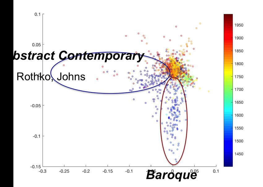
Figure 2: Comparison of the filters learned on object classification vs style classification. Left:
Typical filters of AlexNet trained on ImageNet for object classification. Center and Right: Filters
of AlexNet trained for style classification using 11x11 and 7x7 dim filters.

    Increasing the depth of the network only added no more than 5% to the accuracy from AlexNet
with 5 convolutional layers to ResNet with 152 convolutional layers. In the case for learning from
scratch, increasing the depth did not improve the results where a ResNet with 50 layers performed
worse than an AlexNet with only 5 convolution layers. VGGNet with 13 convolutional layers
performed only 2-3% better than AlexNet. Increasing the depth of VGGNet did not improve the
results. This limited gain in performance with increase in depth, in conjunction with the difference
in the learned filters, suggests that a shallow network might be sufficient for style classification
along with better filter design.

Effect of adding layers with reduced dimensionality:
The experiments showed that adding extra fully connected layers while gradually reducing the
number of nodes in them forces the networks to achieve a “smoother” and more interpretable rep-
resentation. Having a large number of nodes at the fully connected layers allows the representation
to project the data into a very high dimensional space where classification would be easy (specially
in our case with only 20 classes), without necessarily enforcing similar paintings across styles to
come closer in the representation based on their similarity. We quantified this phenomenon by ex-
amining the dimensionality of the subspace of the activation (using Principle Component Analysis
(PCA [14]) of the visualization dataset using two measures: 1) The number of components needed
to preserve 95% of the variance. 2) The variance retained with the first two PCA dimensions. We
also evaluated the accuracy of the expanded models to see if the added reduced layers resulted in
any loss of accuracy. In most of the cased the added layers enhanced the accuracy (see Table 2)
    Table 3 shows that adding two reduced-dimension layers effectively and consistently reduced
the dimensionality of the subspace of the data while preserving the classification accuracy. The
reduction is significant for AlexNet where 9 or 10 dimensions retained 95% of the variance com-
pared to 201 and 397 dimensions for the cases of fine-tuned and learned from scratch networks
respectively, with around 60% of the variance retained in the first two dimension. Interestingly,
the representation achieved by VGGNets already has reduced dimension subspaces compared to

                                                 9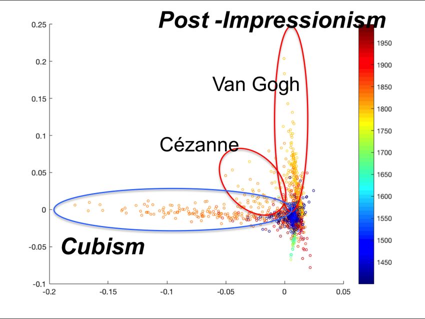
Table 3: The effect of adding two reduced dimension layers on the representation (subspace di-
mensionality and variance)
 Model                  Training Strategy                                                  Original Architecture                                                Adding two dimensionality reduction layers
                                                                number of nodes             subspace dim 1 retained variance 2                              number of nodes subspace dim1 retained variance2
 AlexNet    Pre-trained                                             4096                          201             21.71                                          512              9                59.64
            & Finetuned
 AlexNet From Scratch                 4096                397                 35.62                                                                                         512                                10                 62.78
 VGGNet Pre-trained                   4096                 55                 49.52                                                                                         512                                 7                 66.87
            & Finetuned
 VGGNet From Scratch                  4096                 36                 51.16                                                                                         512                                  7                72.52
 ResNet     Pre-trained               20483               491                 17.53                                                                                         512                                  6                73.71
            & Finetuned
 1 Subspace dim: Number of principle components cumulatively retaining 95% of variance.
 2 Retained variance: Percentage of variance retained by the first two principle components.
 3 ResNet does not have FC layers. This is the number of the nodes in the last pooling layer.

 100
                                                                                                                          100

                                                                                                                                  90

   90

                                                                                              AlexNet+2
  Finetuned
            80

   80
                                                                                                                           70
                                                                                      AlexNet
  Finetuned

                                                                                              AexNet+2
  From
  Scratch

                                                                                                                                  60
                                                                                      AexNet
  From
  Scratch

   70

                                                                                                                                  50

                                                                                              VGG+2
  Finetuned
                                                                                                          VGG
  Finetuned

   60

                                                                                                                                  40

                                                                                                                                                                                                                            VGG
  From
  scratch

   50
                                                                                       VGG+2
  From
  scratch
          30

                                                                                                                                                                                                                            ResNet
  Finetuned

                                                                                                                                  20

   40

                                                                                              ResNet+2
  Finetuned
             10

   30
                                                                                                                             0

            1
     2
     3
     4
     5
     6
     7
     8
     9
   10
                                                      1
     2
     3
     4
      5
     6
     7
     8
     9
   10


Figure 3: Cumulative retained variance by the first 10 PCA dimensions of the activation space at
last FC layer (512 nodes). Left: models after adding the dimensionality reductions layers. Right:
the original models.

the AlexNet and ResNet. However, adding the reduced dimension layers for VGG significantly
lowered the subspace dimension (only 7 dimensions retain 95% of the variance) while improving
its classification accuracy between 2-4%. The maximum reduction in subspace dimensionality was
in ResNet where the dimension of the subspace retaining 95% of the variance was reduced from
491 to only 6 with 74% of the variance in the first two dimensions. Figure 3 shows the cumulative
retained variance for the first 10 PCA dimensions of the activation subspace for all the models
before and after adding the two reduced dimensions layers.

4           Shape of Art History: Interpretation of the Representation
This section focuses on analyzing, visualizing, and interpreting the activation space induced by the
different networks after trained to classify style.
    We define the activation space of a given fully connected layer as the output of that layer prior
to the rectified linear functions. In particular, in this paper, we show the analysis of activation of the
last reduced dimension fully connected layer prior to the final classification layer, which consists
of 512 nodes. We use the activations before the rectified linear functions in all the networks.

                                                                                                                             10
Few Factors Explain the Characteristics of Styles:
The learned representation by the machine shows that there are a few underlying factors that can
explain the characteristics of different styles in art history. Using Principle Component Analysis,
we find that only fewer than 10 modes of variations can explain over 95% of the variance in the
visualization set in all of the studied models with additional reduced fully connected layers. In
ResNet and VGGNet the number of these modes is as low as 6 and 7 respectively. In all of the
networks, the first two modes of variations explained from 60% to 74% from the variance in the
various models in visualization set I (Table 3). Moreover, it is clear from the visualizations of both
the linear and nonlinear embedding of the activation manifold in various models that art dated prior
to 1900 lie on a plane (subspace of dimension 2).
Consistent results are achieved by analyzing the 62K painting from the Wikiart data set where
it was found that subspaces of dimensions 10, 9 and 7 retain 95% of the variance of the activation
for AlexNet+2, VGGNet+2, ResNet+2 respectively (Table 5). The consistency of results in all
the studied networks and the two datasets (varying in size from ≈ 1500 to 62K paintings) imply
that the existence of a small number of the underlying factors explaining the representation is an
intrinsic property of art history, and not just an artifact of the particular dataset or model.
We will start our interpretation of these dimensions by investigating the time correlation with
these dimensions, followed by correlation analysis with Wölfflin’s concepts.
Table 4: Temporal correlation with the first two PCA dimensions and the first LLE dimensions of
the activation space in different models
Pearson correlation coefficient with time
model training 1st PCA dim 2nd PCA dim Radial 1st LLE dim
AlexNet+2 Fine-tuned 0.4554 0.5545 0.6944 0.7101
From scratch -0.5797 0.2829 0.6697 0.6723
VGGNet+2 Fine-tuned -0.2462 0.5316 0.5659 -0.4012
From scratch 0.5781 0.3165 0.6239 -0.6532
ResNet+2 Fine-tuned -0.6559 0.4579 0.7712 0.8130
Smooth Temporal Evolution of Style:
All the learned representations show smooth transition over time. Figure 4 shows the paintings
in the visualization set I, projected into the first two modes of variations of the activations of the
last reduced dimension fully connected layer for different networks. The paintings are color-coded
based on their date of creation. The plots consistently show that the networks learned smooth
temporal representations that reflect the historical progress in style. This is despite the fact that the
networks are trained only with images and their discrete style labels. No information was provided
about when each painting was created, when each style took place, which artist created which
painting, nor how styles are related (such as style x is similar to style y, or came after or before
style z). Despite the lack of all this information, the learned representations are clearly temporally
smooth and reflect high level of correlation with time.
Visualizing these modes of variations reveals very interesting ways of how the networks arrange
the data in a temporal way. For example, for the case of AlexNet+2 model, as shown in Figure 1-A,
11Figure 4: First two modes of variations of different learned representations and their temporal
correlations. Every point is a painting, color-coded by the year of creation. Dataset: VS-I.
the data is arranged in the plot in a radial clock-wise way around the center to make a complete
circle in this 2D projection starting with Renaissance and ending with Abstract Art. We can see
the progress following the plot in a clock-wise way from Italian and Northern Renaissance at
the bottom, to Baroque, to Neo-classicism, Romanticism, reaching to Impressionism at the top
12followed by Post impressionism, Expressionism and Cubism. The cycle completes with Abstract
and Pop Art. The explanation of how the network arranged the representation this way will become
clearer next when we show the results of nonlinear activation manifold analysis.
We quantified the correlation with time in different ways. We measure the Pearson Correlation
Coefficients (PCC) with each of the principle components, as well as with each dimension of
the nonlinear manifold embedding. Table 4 shows the temporal correlation using PCC with the
first two PCA dimensions and the first LLE embedding dimension for different models. We also
computed the correlation of the radial coordinate – of each painting in the projection to the first
two principle components– with time. The temporal correlation obtained in the representation is
consistent among the different networks.
Taking a fine-tuned AlexNet+2 as example, the first two dimensions have very strong correla-
tion with time, 0.46 and 0.55 Pearson correlation coefficients respectively. A linear combination
of these two dimensions with convex weights proportional to their Pearson correlation coefficients
results in a single dimension that has 0.71 correlations with time (Figure 1-B). This cycle around
the plot from Renaissance till abstraction and Pop art suggests that the angular coordinate around
the plot would reflect correlation with time. In fact the angular coordinates have a PCC of 0.69
with time. The strongest temporal correlation is in the case of ResNet with 0.76 PCC radial cor-
relations. This conclusion is consistent among all the networks that we tested. This conclusion
shows that style changes smoothly over time and proves that noisy discrete style labels are enough
for the networks to recover temporal arrangement, due mainly to visual similarities as encoded
through the learned representation in a continuous activation space.
Strong temporal correlation also exists with the modes of variations in Visualization set-II.
However, in this case, it is not necessarily the first two modes of variation that are the ones with
the highest temporal correlation. This is due to the bias in this dataset towards 20th century work.
Table 5 shows the PCC with time for each of the dimensions for three fine tuned networks.
Table 5: Analysis of the modes of variations of the activations on 62K paintings from the Wikiart
collection in three models and their correlation with time (Pearson Correlation Coefficients) . The
top two time-correlated modes are highlighted in bold.
Subspace Dim 1 Retained Variance 2 Correlation with time
1 2 3 4 5 6 7 8 9 10
AlexNet+2 10 51.13 0.12 0.66 0.24 -0.43 -0.23 0.04 0.08 -0.05 -0.03 0.00
VGGNet+2 9 43 -0.15 -0.14 -0.46 -0.07 -0.59 0.28 0.02 0.07 0.02
ResNet+2 7 66.80 -0.03 -0.72 0.20 0.22 0.30 -0.01 0.06
1 Subspace Dim: Number of principle components retaining 95% of the variance
2 Retained Variance: Variance retained by first two dimensions
Interpretation of the Modes of Variations - Relation to Wölfflin’s Pairs:
Visualizing the modes of variations reveals very interesting ways of how the networks were able to
consistently capture evolution and characteristics of styles. Here we take the fine-tuned AlexNet+2
as example, however similar results can be noticed in other models. The first mode (the horizontal
axis in Figure 1) seems to correlate with figurative art, which was dominant till Impressionism,
vs. non-figure, distorted figures, and abstract art that dominates 20th century styles. Another
interpretation for this dimension is that it reflects Wölfflin’s concept of planar (to the right) vs.
13recession (to the left). This axis correlates the most with Wölfflin’s concept of planar vs recession
with -0.50 Pearson correlation coefficient. To a lesser degree, this horizontal axis correlates with
closed vs. open (0.24 PCC) and linear vs. painterly (-0.23 PCC). This quantitative correlation can
be clearly noticed by looking at the sampled paintings shown in Figure 1, where we can see that
the horizontal axis is characterized by planar, open, and linear form to the right (as in Cubism,
and Abstract) vs. recession, closed, and painterly to the left (as appears in some of the Baroque
paintings at the extreme left)
Table 6: Correlation with Wölfflin’s concepts. Pearson Correlation Coefficient of the first two PC
dimensions and the first two LLE dimensions of the activation space and Wölfflin’s concepts. The
concepts with maximum correlation with each dimension are shown.
Pearson correlation coefficient(absolute values) with Wölfflin’s concepts
Model Training 1st PCA dim 2nd PCA dim 1st LLE dim 2nd LLE dim
Planar vs. Linear vs. Planar vs. and Linear vs.
Recession Painterly Recession Painterly
AlexNet+2 Fine-tuned 0.4946 0.3579 -0.501 0.3216
From scratch 0.5129 0.3272 0.4930 -0.3111
VGGNet+2 Fine-tuned 0.3662 0.2638 0.4512 0.2646
From scratch 0.4621 0.4000 0.4897 0.3174
ResNet+2 Fine-tuned 0.5314 0.4795 0.5251 0.4158
The second mode of variations (the vertical axis) has 0.36 Pearson correlation coefficient with
the linear (towards the bottom) vs. painterly (towards the bottom) concept. We can clearly see
the smooth transition from linear form in Renaissance at the bottom towards more painterly form
in Baroque to the extreme case of painterly at Impressionism at the top. Then we can see the
transition back to linear form in abstract and Pop art styles. Projecting the data into these two
dominant modes of variations, which are aligned with plane vs. recession and linear vs. painterly,
gives an explanation to why this representation correlates with time in a radial fashion.
The correlation between the first two modes of variations and the concepts of planar vs. re-
cession and linear vs. painterly is consistent among all the representations learned by all tested
networks, whether pre-trained or trained from scratch. In all cases the first mode of variations cor-
relates the most with the concept of planar vs. recession while the second mode correlates the most
with linear vs. painterly. Table 6 shows the Pearson correlation coefficients with these concepts.
Full correlation results with all dimensions are shown in the appendix.
The fourth and fifth dimensions of AlexNet+2 representation spread away strongly the Renais-
sance vs Baroque styles and put other styles in perspective to them (Figure 5). The fifth dimension
in particular (and the fourth dimension to a lesser degree) correlates with relative vs. absolute
clarity, unity vs. multiplicity, open vs. closed, and painterly vs. linear form from top to bottom
(with PCC 0.36, 0.30, 0.28, 0.16 respectively). This is consistent with Wölfflin’s theory since
he suggested exactly the same contrast between these concepts to highlight the difference between
Renaissance and Baroque. In Figure 5-A , the Renaissance style appears at the top (absolute clarity,
multiplicity, closed, linear form) while the Baroque appears at the bottom (relative clarity, unity,
and open, painterly form). We can see in the figure that Impressionism and Cubism are at the top
half of the plot since they share many of these same concepts with Baroque. The fourth dimension
seems to separate Impressionism and Cubism to the right from abstraction and Pop art to the left.
14A
Van Eyck Durer Van Eyck Van Eyck Mantegna Da Vinci
Rousseau
Raphael
Rousseau Warhol
Raphael
Klimt
Warhol
Da Vinci
Lichtenstein
Sisley
Goya
Monet
Picasso
Braque
Vermeer Delacroix Rembrandt Velázquez Renoir
B
0.3%
0.2%
0.1% Linear%vs%Painterly%
Close%vs%Open%
0%
4% 5% Planer%vs%Recession%
!0.1%
Mul>plicity%vs%Unity%
!0.2% Absolute%vs%Rela>ve%Clarity%
!0.3%
!0.4%
Figure 5: Separation between Renaissance and Baroque: (A) The fourth and fifth modes of vari-
ations show separation between Renaissance and Baroque. (B) Correlation between these two
modes of variations and Wölfflin’s concepts, which confirms with Wölfflin’s hypothesis.
Looking at the 4th, 5th, and 6th dimensions of the embedded activation manifold, we can notice
two orthogonal planes characterizing art prior to 1900 (Figure 10). One plane spans Renaissance
vs. Baroque while an orthogonal plane spans Impressionism vs. Post-Impressionism.
15A Renoir
Rothko
Monet
Impressionism
Van Gogh Johns
Mondrain Raphael
Cézanne
Post -Impressionism
Baroque
Cubism
Rousseau
Rembrandt
Picasso
Northern Renaissance
Velazquez
Durer
Van Eyck
B C D E
Rubens
Impressionism
Baroque
Pop Art
Naïve art/Primitivism
Rousseau
F G H
Figure 6: The representation could discover distinctive artists for each style. (A)The first three modes
of variations of the VGGNet activations. Distinctive artists representing each style are identified by the
representation and pulled away from the cloud at the center. (B-E) Factorization of the activation space
using Independent Component Analysis into 7 maximally independent axes, which show alignment with
styles (more details in Figure 7). (F-H) The top three modes of variations in the VGG network activation
of 62K works of art from the Wikiart collection (projected pairwise as dimensions 1-2, 2-3, 3-1 from left to
right).
16Discovering Limitations of Wölfflin’s Concepts:
Interestingly, not all modes of variations explaining the data correlate with Wölfflin’s concepts. In
all learned representations, one of the first five modes of variation always has close-to-zero linear
correlation with all Wölfflin’s concepts. A notable example is the fifth dimension of the embedded
activation manifolds, which separates Impressionism from Post-Impressionism, and has almost
zero linear correlation with Wölfflin’s pairs (Figure 10). This implies that the separation between
these styles is not interpretable in terms of Wölfflin’s pairs.
Identification of Representative Artists:
Visualizing the different representations shows that certain artists were consistently picked by the
machine as the distinctive representatives of their styles, as they were the extreme points along
the dimensions aligned with each style. This is visible in the first three modes of variations of the
representation learned by the VGGNet, shown in Figure6-A, which retains 77% of the variance .
Besides the observable temporal progress, the representation separates certain styles and certain
artists within each style distinctively from the cloud at the center as non-orthogonal axes.
We can see the Northern Renaissance in the yellow ellipse with the majority of the paintings
sticking out being by Van Eyck and Dürer. The Baroque in the black ellipse is represented by
Rubens, Rembrandt, and Velzquez. The orange ellipse is Impressionism and at its base are Pissarro,
Caillebotte, and Manet as the least painterly of the type, ending with Monet and Renoir as most
painterly on the end of the spike. The two red circles are Post-Impressionism, and in particular
one is dominated by Van Gogh, and the other by Cézanne who forms the base for the spike of
Cubism in the light blue ellipse. This spike is dominated by Picasso, Braque, and Gris; and goes
out to the most abstract Cubist works. Most interestingly the representation separates Rousseau, as
marked in the green ellipse, which is mainly dominated by his work. Consistent results can be seen
when plotting the embedding of the activation of the whole 62K paintings in the Wikiart dataset
collection as can be seen in Figure 6 F-H.
Applying Independent Component Analysis (ICA) [15, 17] to the activation space results in
finding non-maximally independent non-Gaussian orthogonal axes3 . Figure 6 B-E shows the ICA
factorization of the VGG network activation space. Here, the same subspace that retains 95% of
the variance is factorized by ICA. This results in 7 maximally independent components shown in
Figure 6-E.
We also show each of these components against the time axis in Figure 7. Some components
are aligned with specific styles (A: Baroque, C: Cubism, D: Post-Impressionism, E: abstract art, F:
Renaissance) and other components contrast several styles (B and F). This factorization facilitates
quantitatively discovering the artists who represent each style, as their works appear as the extreme
points on the axes of each style. It also highlights which styles are opposite to each other along
each of these axes 4 .
3
Independent Component Analysis (ICA) transforms activation to a new embedding space in which transformed
data become statistically independent as much as possible and the ICA achieve this by finding non-orthogonal basis in
original activation space maximizing independence criteria.
4
Since the ICA algorithm (Fast ICA [17]) used in this experiment has a limitation to capture over-completeness,
which implies existence greater number of fat tails than dimension of the space, our experiment found only some of
axes are aligned with styles. However, still the results show that ICA has merits to find some of interesting art historical
facts and provide quantitatively measurement of them, such as what art works or which artists are most representative
17A B Impressionism C
Cubism
Lichtenstein
Baroque Van Eyck Durer Rousseau
Warhol
D Post Impressionism E F
Abstract art Renaissance
G H 0.4%
0.3% Linear%vs%Painterly%
0.2% Close%vs%Open%
0.1%
Planer%vs%Recession%
0%
1% 2% 3% 4% 5% 6% 7% Mul@plicity%vs%Unity%
!0.1%
Rothko, Absolute%vs%Rela@ve%
Raphael El-Greco !0.2% Clarity%
Johns !0.3%
Figure 7: Independent component factorization of the activation of VGG network representation
achieved by ICA. A-G: Each independent component vs time (1400-2000AD). H: Correlation
(PCC) with Wölfflin’s concepts. Some components are aligned with specific styles (A: Baroque,
C: Cubism, D: Post-Impressionism, E: abstract art, F: Renaissance) and other components contrast
several styles (B and G).
The fact that the representation highlights a certain representative artist or artists for each style –
among hundreds or thousands of paintings by many artists in each style – emphasizes quantitatively
the significance of these particular artists in defining the styles they belong to.
Interpretations of the Activation Manifold and Understanding Influences:
Using nonlinear dimensionality reduction of the activation allows us to achieve an embedding of
the activation manifold of the visualization data sets, which reveals interesting observations as
well. In particular we used Local Linear Embedding (LLE) [16]. LLE, as other similar techniques,
is based on building a graph of data points, where each point is connected to its nearest neighbors,
and using such graph to embed the data to a low dimensional space where it can be visualized. In
our case the data points are the activation of a given painting as it goes through the deep network,
and measured at the last fully connected layer, and this results in an embedding of the activation
within each of styles.
18manifold. Controlling the number of neighbors of each painting in constructing the graph allows
for controlling connections between paintings. If this parameter is set to a small number, this
results in accentuating distinctive paintings and trends. If we set this parameter to a large number,
we allow more paintings to connect and we can capture the overall trend.
The first dimension of the LLE representation of all the models exhibits strong temporal cor-
relation, as shown in Table 4. For example, the first LLE dimension in AlexNet+2 representation
has 0.71 PCC with time that of ResNet+2 has 0.81 PCC with time. Also, similar to the modes of
variations, the first two LLE dimensions shows strong correlation with Wölfflin’s concepts planar
vs. recession and linear vs. painterly respectively, see Table 6. Looking at the representation
learned by AlexNet+2, as an example, we can notice that on the surface of the embedded acti-
vation manifold, different styles are arranged in the learned representation in a way that reflects
their temporal relation as well as stylistic similarity (see Figure 8-A)5 . The temporal relation be-
tween styles is not just linear historical order, since elements of some styles can appear later in
other styles. For example we can see linear temporal progress from Renaissance, to Baroque, to
Romanticism, to Realism to Impressionism. However we can also see direct connection between
Renaissance to Post-Impressionism and 20th century styles. This can be explained since the use of
linear (vs. painterly) and planar (vs. recessional) concepts in these later styles echo these elements
from Renaissance style(Fig 8-B).
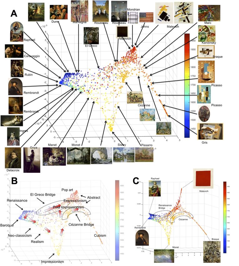
One interesting connection that is captured in this representation is the arrangement of Cézanne’s
work in a way that connects Impressionism to Cubism. We can clearly see in Figures 8-B and 9-
A that Cézanne’s work acting as a bridge between Impressionism at one side and Cubism and
Abstract at the other side. Art historians consider Cézanne to be a key figure in the style transi-
tion towards Cubism and the development of abstraction in the 20th century art. This bridge of
Cézanne’s painting in the learned representation is quite interesting because that is a quantifiable
connection in the data, not just a metaphorical term. We can see branching at Post-Impressionism
where Cézanne’s work clearly separates from the other Post impressionist and expressionist works
towards the top. This branch continues to evolve until it connects to early Cubist works by Picasso
and Braque, as well as abstract works by Kandinsky.
Figures 8-B and 9-B show another interesting connection between the Renaissance and mod-
ern art as captured by the learned representation. Despite the fact that the structure reflects smooth
temporal progression, it is interesting to see outlier to this progression. In particular there are some
High Renaissance, Northern Renaissance and Mannerist paintings that stick out of the Renaissance
cluster to the left and connect to art from late 19th and early 20th centuries. This is because fre-
quent similarity between art works across time results in pulling influential works of art out of
order and placing them closer to the art they may have influenced. We can see in the figure that
the works that stick out of the Renaissance cluster at the left and connect to modernity are mainly
dominated by some paintings by El-Greco and some paintings by Dürer. Among the paintings by
El-Greco that significantly stick out are Laocoön, Saint Ildefonso, View of Toledo, and Pietà. We
can also see works by Raphael, Mantegna, and Michelangelo in this group as well.
We can accentuate this representation by the reducing the number of neighbors of each paint-
ing while constructing the manifold. This small neighborhood construction results in lining up
distinctive paintings in thin structures to accentuate trends. This results of this version shown in
5
The representation is achieved by setting the neighborhood size to 100 to capture the overall trend.
19Figure 8: Interesting connections discovered in the activation manifold. (A) Example of activation
manifold of AlexNet+2. Paintings color coded by date on the surface of the activation manifold
showing smooth transition over time. (B) Transitions between art movements and important con-
nections. (C) Accentuated version of the manifold highlighting five major styles: Renaissance,
Baroque, Impressionism, Cubism, and abstract.
20Figure 9: Interesting connections. (A) Cézanne’s bridge: we can see branching at Post-
Impressionism where Cézanne’s work clearly separates from the other Post-Impressionist and Ex-
pressionist works towards the top. This branch continues to evolve till it connects to early Cubist
works by Picasso and Braque, as well as abstracts works by Kandinsky. All thumbnails without
labels in this plot are by Cézanne. (B) The connection between Renaissance and modern styles
is marked by the outliers in the temporal progress patterns by certain works by El-Greco, Dürer,
Raphael, Mantegna, and Michelangelo.
Figure 8-C6 . In this visualization, five distinct styles are clearly accentuated among all the twenty
styles that the machine learned: Renaissance, Baroque, Impressionism, Cubism, and Abstract. We
show the representative paintings at the tip of each of the five styles, which are in order Raphael’s
St. Catherine (1507), Rembrandt’s self-portrait (1640), Monet’s Water Lilies under clouds (1903),
Braque’s Violin and Candlestick (1910), and Malevich’s Red Square (1915). Both Cézanne’s
bridge and El-Greco/Dürer’s bridge are accentuated in this representation as well.
Interestingly, both Cézanne’s connection and El-Greco/Dürer connection appears consistently
in the various representations learned by different networks, however manifested in different forms.
Another interesting observation is that Cubism appears as very unique style that sticks out of as a
singularity in most of the representations.
5 Conclusions and Discussion
In this paper we presented the result of a comprehensive study of training various deep convolu-
tional neural networks for the purpose of style classification. We mainly emphasized analyzing the
learned representation to get an understanding of how the machine achieves style classification.
The different representations learned by the machine using different networks shared striking
similarities in many aspects. It is clear that a small numbers of factors can explain most of the
6
The accentuated representation is achieved by setting the neighborhood size to 25 to reduce the connectivity and
accentuate the visualization.
21A B
Impressionism
Renaissance
Baroque
Post-Impressionism
C D
Baroque Baroque
Impressionism Post-Impressionism
0.3%
E
0.2%
Linear%vs%Painterly%
0.1%
Close%vs%Open%
Planer%vs%Recession%
0%
4% 5% 6%
Mul?plicity%vs%Unity%
!0.1%
Absolute%vs%Rela?ve%
Clarity%
!0.2%
!0.3%
Figure 10: Two orthogonal planes characterize art prior to 1900 in the learned Representation.
Renaissance-Baroque plane seems orthogonal to the Impressionism-Post-Impressionism plane in
the embedding of the activation manifold of fine-tuned AlexNet+2 model is shown. (A,B) Two
different view of the 4th, 5th, 6th dimensions are shown. (C) the 4th and 6th dimensions span
the Renaissance-Baroque differences. (D) 5th and 6th dimensions. The 5th dimension spans the
Impressionism-Post-Impressionism differences. Interestingly, the 5th dimension has very small
correlation with Wölfflin’s concepts. (E) Correlation with Wölfflin’s concepts
22variance in the studied datasets in all the trained models (between 7 and 10 factors explains 95%
of the variance), which indicates that a small number of factors encapsulate the characterization of
different styles in art history.
The results also indicate that the learned representation shows a smooth temporal transition be-
tween styles, which the machine discovered without any notion of time given at training. Most
interestingly, studying the modes of variations in the representation showed a radial temporal
progress, with quantifiable correlation with time, starting at Renaissance, to Baroque, progress-
ing all the way to Impressionism, Post impression, Cubism and closing the loop with 20th century
styles such as Abstract and Pop Art coming back close to Renaissance. By studying the correlation
between the modes of variations and Wölfflin’s suggested pairs, it was found that, consistently, all
the learned models have the first mode of variation correlating the most with the concept of plane
vs. recession while the second mode of variation correlates the most with the concept of linear
vs. painterly. This correlation explains the radial temporal progress and the loop closure between
Renaissance and 20th century styles since they share linearity and planarity in their form.
We also studied the activation manifold of the different representation learned by the machine,
which also reveal smooth temporal progress captured by the representation as well as correlation
with Wölfflin’s concepts. Studying the activation manifolds with different neighborhood structure
allowed us to discover different interesting connections in the history of art in a quantifiable way,
such as the role of Cézanne’s work as a bridge between a Impressionism and Cubism-Abstract
art. Another interesting connection is the connection between Renaissance and modern styles such
as Expressionism, Abstract-Expressionism, through the works of El-Greco, Dürer, Raphael, and
others.
Visualizing the different representations shows that certain artists were consistently picked by
the machine as the distinctive representatives of the styles they belong to as they were the extreme
points along the dimensions aligned with each style. For example, such distinctively representa-
tive artists are Van Eyck and Dürer for Northern Renaissance, Raphael for Italian Renaissance,
Rembrandt and Rubin for Baroque, Monet for Impressionism, Cézanne and Van Gogh for Post
Impressionism, Rousseau for Nave-Primitivism, Picasso and Braque for Cubism, and Malevich
and Kandinsky for Abstract. While this is quite known for art historians, the machine discovered
and highlighted these artists, amongst many others in each style, as the distinctive representatives
of their styles without any prior knowledge and in a quantifiable way.
The networks are presented by raw colored images, and therefore, they have the ability to
learn whatever features suitable to discriminate between styles, which might include composi-
tional features, contrast between light and dark, color composition, color contrast, detailed brush
strokes, subject matter related concepts. In particular, networks pre-trained on object categoriza-
tion datasets might suggest potential bias towards choosing subject-matter-related features for clas-
sification. However, visualizing the learned representations reveals that the learned representations
rule out subject matter as a basis for discrimination. This is clear from noticing the loop closure
between Renaissance style, which is dominated with religious subject matter, and modern 20th
century styles, such as Abstract, Pop art, and others. In contrast, this loop closure suggests that the
basis of discrimination is related to concepts related to the form as suggested by Wölfflin.
The implication of the networks ability to recover a smooth temporal progression through the
history of art, in absence of any temporal cues given at training, and in absence of any temporal con-
straints other than putting paintings of the same style closer to each other to achieve classification,
suggests that visual similarity is the main factor that forces this smooth temporal representation to
23You can also read