TimeSpec4LULC: a global multispectral time series database for training LULC mapping models with machine learning
←
→
Page content transcription
If your browser does not render page correctly, please read the page content below
Earth Syst. Sci. Data, 14, 1377–1411, 2022
https://doi.org/10.5194/essd-14-1377-2022
© Author(s) 2022. This work is distributed under
the Creative Commons Attribution 4.0 License.

            TimeSpec4LULC: a global multispectral time series
             database for training LULC mapping models with
                             machine learning
              Rohaifa Khaldi1,2,4 , Domingo Alcaraz-Segura2,3,5 , Emilio Guirado6 , Yassir Benhammou1,7 ,
                             Abdellatif El Afia4 , Francisco Herrera1 , and Siham Tabik1
        1 Department   of Computer Science and Artificial Intelligence, Andalusian Research Institute in Data Science
                    and Computational Intelligence (DaSCI), University of Granada, 18071, Granada, Spain
                  2 Department of Botany, Faculty of Science, University of Granada, 18071 Granada, Spain
                    3 Andalusian Center for the Assessment and Monitoring of Global Change (CAESCG),

                                          University of Almería, 04120, Almería, Spain
                                 4 ENSIAS, Mohammed V University, Rabat, 10170, Morocco
        5 iEcolab, Inter-University Institute for Earth System Research, University of Granada, 18006 Granada, Spain
                            6 Multidisciplinary Institute for Environment Studies Ramón Margalef,

                                University of Alicante, San Vicente del Raspeig, 03690, Spain
                                     7 ENSA, Hassan I University, Berrechid, 218, Morocco

           Correspondence: Rohaifa Khaldi (rohaifa@ugr.es) and Domingo Alcaraz-Segura (dalcaraz@ugr.es)

                                  Received: 26 July 2021 – Discussion started: 12 October 2021
                       Revised: 3 February 2022 – Accepted: 14 February 2022 – Published: 30 March 2022

      Abstract. Land use and land cover (LULC) mapping are of paramount importance to monitor and understand
      the structure and dynamics of the Earth system. One of the most promising ways to create accurate global
      LULC maps is by building good quality state-of-the-art machine learning models. Building such models re-
      quires large and global datasets of annotated time series of satellite images, which are not available yet. This
      paper presents TimeSpec4LULC (https://doi.org/10.5281/zenodo.5913554; Khaldi et al., 2022), a smart open-
      source global dataset of multispectral time series for 29 LULC classes ready to train machine learning models.
      TimeSpec4LULC was built based on the seven spectral bands of the MODIS sensors at 500 m resolution, from
      2000 to 2021, and was annotated using spatial–temporal agreement across the 15 global LULC products avail-
      able in Google Earth Engine (GEE). The 22-year monthly time series of the seven bands were created globally
      by (1) applying different spatial–temporal quality assessment filters on MODIS Terra and Aqua satellites; (2) ag-
      gregating their original 8 d temporal granularity into monthly composites; (3) merging Terra + Aqua data into a
      combined time series; and (4) extracting, at the pixel level, 6 076 531 time series of size 262 for the seven bands
      along with a set of metadata: geographic coordinates, country and departmental divisions, spatial–temporal con-
      sistency across LULC products, temporal data availability, and the global human modification index. A balanced
      subset of the original dataset was also provided by selecting 1000 evenly distributed samples from each class
      such that they are representative of the entire globe. To assess the annotation quality of the dataset, a sample of
      pixels, evenly distributed around the world from each LULC class, was selected and validated by experts using
      very high resolution images from both Google Earth and Bing Maps imagery. This smartly, pre-processed, and
      annotated dataset is targeted towards scientific users interested in developing various machine learning models,
      including deep learning networks, to perform global LULC mapping.

Published by Copernicus Publications.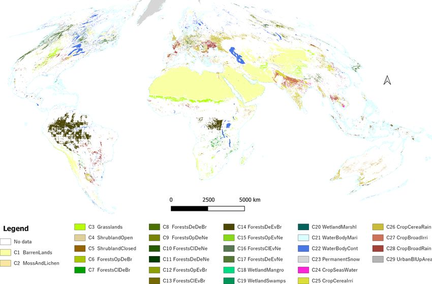
1378                                                                                           R. Khaldi et al.: TimeSpec4LULC

1   Introduction                                                    face from regional to global scales (Kong et al., 2016; Kerr
                                                                    and Ostrovsky, 2003; Pfeifer et al., 2012) thanks to their
Broadly, land cover (LC) refers to the different vegetation         strong ability to cover, timely and repeatedly, wide and in-
types (usually following biotype, plant functional type, or         accessible areas, as well as to get high spatial and temporal
physiognomy schemes, such as forests, shrublands, or grass-         resolution data (Alexakis et al., 2014; Yirsaw et al., 2017;
lands) or other biophysical classes (such as water bodies,          Patel et al., 2019).
snow, or bare soil) that cover the Earth’s surface (Moser,              Deep learning (DL), a sub-field of machine learning essen-
1996). Land cover is an essential variable that provides pow-       tially based on deep artificial neural networks (Zhang et al.,
erful insights for the assessment and modeling of terres-           2018c), has shown impressive performance in computer vi-
trial ecosystem processes, biogeochemical cycles, biodiver-         sion and promising ones in remote sensing during the last
sity, climate, and water resources, among others (Luoto et al.,     decades. Currently, two specific types of DL models, i.e.,
2007; Menke et al., 2009; Polykretis et al., 2020), whereas         CNNs (convolutional neural networks) and RNNs (recurrent
land use (LU) incorporates many types of modifications that         neural networks), constitute the state of the art in respectively
an increasing human population, more than 9 billion ex-             extracting spatial and temporal/sequential patterns from data
pected by 2050, causes to the LC (such as urban areas and           records. Indeed, DL models are showing great performance
croplands). Accurate LULC information, including distribu-          in LULC tasks such as scene classification (Zhang et al.,
tion, dynamics, and changes, is of paramount importance for         2018a), object detection (Zhao et al., 2015; Guirado et al.,
understanding and modeling the natural and human-modified           2021), and segmentation (Zhao and Du, 2016; Guirado et al.,
behavior of the Earth’s system (Tuanmu and Jetz, 2014; Ver-         2017; Safonova et al., 2021) in RGB and multispectral satel-
burg et al., 2009).                                                 lite and aerial images. However, such good performance is
   LULCs are subjected to anomalies, trends, and changes            only possible when DL models are trained on smart data.
both from anthropogenic and natural origins (Polykretis             The concept of smart data involves all pre-processing meth-
et al., 2020). LULC change is usually interpreted as the            ods that improve value and veracity of data and of associ-
conversion from one LULC category to another and/or the             ated expert annotations (Luengo et al., 2020), resulting in
modification of land management within LULC (Meyer and              high-quality and accurately annotated datasets. In general,
Turner, 1994). LULC is an essential climate and biodiver-           remote sensing datasets contain noise, missing values, and
sity variable (Bojinski et al., 2014; Pettorelli et al., 2016) to   high variability and complexity across space, time, and spec-
model and assess the status and trends of social–ecological         tral bands. Applying pre-processing methods, such as gap
systems from the local to the global scale in the pursuit of a      filling and noise reduction to data, and consensus across mul-
safe operating space for humanity (Steffen et al., 2015). For       tiple sources to annotations contribute to creating smart re-
example, characterizing such LULC changes is critical for           mote sensing datasets.
the climate through two mechanisms: biophysical (BPH) and               Currently, there only exist few multispectral datasets an-
biogeochemical (BGC) feedbacks (Duveiller et al., 2020).            notated for training DL models to map LULC and monitor
For instance, the conversion from forests to croplands (i.e.,       their change (Table 1). However, most of these datasets pro-
deforestation) generates a fast increase in land surface tem-       vide very short time series of data, provide very few LULC
perature (i.e., biogeophysical effect) and also releases part       classes, and do not have a global coverage. As far as we
of the carbon stored in the forest into the atmosphere (i.e.,       know, there is no dataset designed for DL models that al-
biogeochemical component). Both mechanisms contribute to            lows global-scale analysis of many LULC classes using long-
local and global warming, respectively (Oki et al., 2013).          time-series data.
Other examples of LULC conversion are urban sprawl, agri-               This paper presents TimeSpec4LULC, a new open-source,
culture expansion, or abandonment, which also affect the            smart, and global dataset of multispectral time series targeted
biodiversity, soil and water quality, food security, and hu-        towards the development and evaluation of DL models to
man health among many others (Lambin and Geist, 2008;               globally map LULCs. TimeSpec4LULC was built using GEE
Feddema et al., 2005). For these reasons, continuous and            (Gorelick et al., 2017) by combining the seven 500 m spectral
accurate LULC and LULC change mapping is essential in               bands of MODIS Aqua and MODIS Terra satellite sensors at
policy and research to monitor ecological and environmen-           a monthly time step from 2000 to 2021. It contains millions
tal change at different temporal and spatial scales (Polykretis     of pixels that were annotated based on a spatial–temporal
et al., 2020; García-Mora et al., 2012) and as a decision sup-      consensus across up to 15 global LULC products (Table 2)
port system to ensure an effective and sustainable planning         for 29 broad and globally harmonized LULC classes. In ad-
and management of natural resources (Kong et al., 2016;             dition, it provides metadata at pixel level: geographic coordi-
Congalton et al., 2014; Grekousis et al., 2015).                    nates, country and departmental divisions, spatial–temporal
   Satellite remote sensing in combination with geographic          consistency across LULC products, statistics on temporal
information systems (GISs) has provided convenient, inex-           data availability, and the global human modification index.
pensive, and continuous spatial–temporal information for            The annotation quality was further assessed by experts using
mapping LULCs and detecting changes on the Earth’s sur-             Google Earth and Bing Maps very high resolution images

Earth Syst. Sci. Data, 14, 1377–1411, 2022                                          https://doi.org/10.5194/essd-14-1377-2022
R. Khaldi et al.: TimeSpec4LULC                                                                                               1379

using 100 samples per class evenly distributed around the                amount of complementary information that can help to
world.                                                                   differentiate among LULC classes.
                                                                      – Processing techniques. The different algorithms for at-
2     Methods                                                           mospheric correction, cloud filtering, image composi-
                                                                        tion, viewing geometry corrections, etc., can also influ-
To build TimeSpec4LULC, we first determined the spatial–                ence LULC accuracy.
temporal agreement across 15 heterogeneous global LULC                – Acquisition year(s). Some LULC products just refer to
products (listed in Table 2) for 29 broad and globally harmo-           a particular year, while others are regularly updated.
nized LULC classes. Then, for each class, we extracted a 22-
year monthly time series for the seven 500 m spectral bands           – Classification schemes. LULC legends can greatly dif-
of MODIS Terra and Aqua combined. We carried out this                   fer in the number of classes and typology definitions. In
process in GEE since it provides access to freely available             general, LULC products tend to agree more in broader
satellite imagery under a unified programming, processing,              general categories than in finer specific ones.
and visualization environment.                                        – Classification algorithms. The approaches and rules
                                                                        used to identify each LULC have evolved from deci-
2.1    Finding spatial–temporal agreement across 15                     sion trees to multivariate clustering and machine learn-
       global LULC products                                             ing, including now deep learning.
                                                                      – Validation techniques of the final product. The amount
Since the 1980s, multiple global LULC products (Table 2)
                                                                        and global distribution of ground truth samples differ
have been derived from remotely sensed data, providing al-
                                                                        across products and influence their reported accuracy.
ternative characterizations of the Earth surface at varying ex-
tents of spatial and temporal resolutions (Townshend et al.,        Many efforts have been made to assess, compare, and har-
1991; Loveland et al., 2000; Bartholome and Belward, 2005).         monize the increasing plethora of global, regional, and lo-
One of the most important limitations of global LULC prod-          cal LULC products, including their integration into synthetic
ucts is the within-product variability of accuracy (across dif-     products, which has shed light onto their strengths and weak-
ferent years, regions, and LULC types) and the low agree-           nesses (Feng and Bai, 2019; Zhang et al., 2019; Gao et al.,
ment among products in many regions of the world (Tsend-            2020; Liu et al., 2021). Still, the myriad of existing products
bazar et al., 2015b, 2016; Gao et al., 2020; Gong et al.,           with different specifications and accuracies have made their
2013; Zimmer-Gembeck and Helfand, 2008). The accuracy               selection by the users problematic and discouraging because
of the global products at the local level is low compared to        it is frequently unknown whether a product meets the user’s
their accuracy at the global level and to the accuracy of lo-       needs for a particular area or LULC class (Tsendbazar et al.,
cal products at the local level. Such lack of consensus can         2015b; Xu et al., 2020). In addition, many of these efforts are
translate into huge implications for subsequent global as-          either limited to regional or national scale (e.g., Pérez-Hoyos
sessments of biodiversity status, carbon balance, or climate        et al., 2012; Gengler and Bogaert, 2018), coarse spatial reso-
change (Estes et al., 2018; de la Cruz et al., 2017). In addi-      lution (e.g., Tuanmu and Jetz, 2014; Jung et al., 2006), or just
tion, accuracy at the local level can be too low, which im-         one LULC type (e.g., Fritz et al., 2011). The use of synergis-
pedes the use of global or regional LULC products in lo-            tic products takes advantage from the strengths of individ-
cal studies (Hoskins et al., 2016; Tsendbazar et al., 2016),        ual products while attenuating their respective weaknesses.
since it can lead to different conclusions due to the com-          However, they still face the challenge of taking into consider-
pelling amount of inconsistencies, uncertainties, and inaccu-       ation the spatial–temporal consistency within pixels. In gen-
racies (Tsendbazar et al., 2015a; Estes et al., 2018). Multiple     eral, given a target maximum error of 5 %–15 % either per
reasons lie behind these discrepancies among LULC prod-             class or for the overall accuracy, most of the current global
ucts (Congalton et al., 2014; Grekousis et al., 2015; Gómez         land cover maps still do not meet the accuracy demands of
et al., 2016).                                                      many applications (Liu et al., 2021).
                                                                        To overcome all the aforementioned limitations, a spatial–
    – Satellite sensors. The spatial, temporal, and spectral res-   temporal agreement across 15 global LULC products avail-
      olutions of the source satellite images strongly deter-       able in GEE was performed. To find the spatial–temporal
      mine the precision and accuracy of derived LULCs. Na-         consensus across global LULC products for different LULC
      tive pixel size can vary from dozens of meters to kilo-       classes, we followed five steps: (1) selection of global
      meters, which determines the precision. Revisiting fre-       LULC products, (2) standardization and harmonization of
      quency can vary from daily images to several weeks,           LULC legends, (3) combination of products across space and
      which determines the possibility of removing cloud and        time, and (4) reprojection and selection of spatial agreement
      atmospheric noise effects. In addition, the greater the       thresholds to get a final consistent mask across the 15 prod-
      number of spectral bands in a sensor, the greater the         ucts for each one of the 29 LULC classes.

https://doi.org/10.5194/essd-14-1377-2022                                          Earth Syst. Sci. Data, 14, 1377–1411, 2022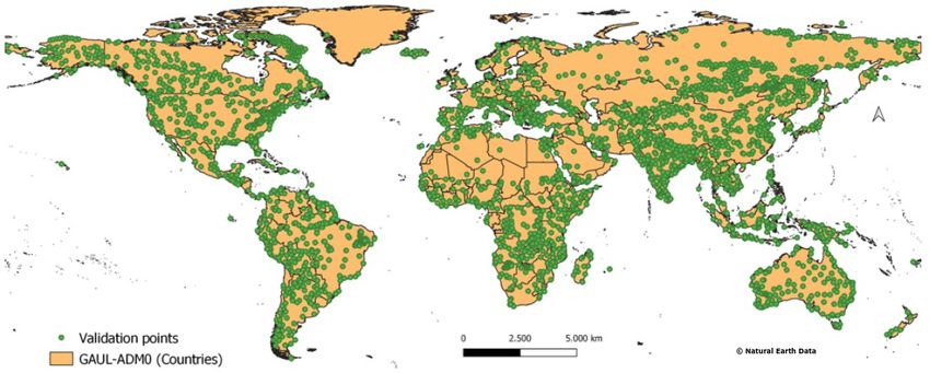
1380                                                                                                                     R. Khaldi et al.: TimeSpec4LULC

Table 1. A list of existing datasets of times series of satellite images, including the proposed TimeSpec4LULC dataset, for training machine
learning models.

 Dataset             Source        No. images × (pixels)           Spatial   Temporal          No.      No.    Extent            Intra/inter-     Labeled
                                                           resolution (m)    resolution      bands   classes                     time series      for
 CaneSat             Sentinel-2    1627 × (10 × 10)                    10    Monthly             6        2    India             [2018, 2019]     Sugarcane clas-
 (Virnodkar                                                                                                                                       sification
 et al., 2020)
 SpaceNet-7          Dove           24 × (1024 × 1024)                  4    Monthly             8        2    100 cities        [2017, 2020]     Buildings
 (Van        Etten   satellite                                                                                                                    tracking
 et al., 2021)       constellation,

                     Planet
                     Labs
 Time       series   MODIS         21 129 pixels                      250    8 d intervals      4        19    France            [2006, 2017]     Crop type map-
 spectral dataset    and LPIS                                                                                                                     ping and moni-
 for croplands in                                                                                                                                 toring
 France
 (Hubert-Moy
 et al., 2019)
 TiSeLaC (TiS,       Landsat       8 × (2866 × 2633)                   30    Annually           10        9    Réunion           2014             Classification
 2022)
 BreizhCrops         Sentinel-2    610 000 pixels                      60    –                  10        9    Brittany dept.,   [1 Jan 2017,     Crop type map-
 (Rußwurm                                                                                                      France            31 Dec 2017]     ping
 et al., 2019)
 TimeSpec4LULC MODIS               6 076 531 pixels                   500    Monthly             7       29    Global            [Mar 2000, Dec   LULC mapping
                                                                                                                                 2021]
 (ours)

2.1.1      Selection of global LULC products                                            classes. Table A2, in Appendix, provides the detailed defini-
                                                                                        tions of each one of the 29 classes from the definitions given
We used the 15 most updated global LULC products avail-                                 in the original products.
able in GEE (Table 2). These products widely differ in their                               The LULC legend was structured into six hierarchical lev-
source satellite data, spatial resolution, temporal coverage,                           els (L0 to L5). The six anthropogenic LU classes contained
class legend, and accuracy. Given such heterogeneity, we                                urban and built-up areas and five types of croplands. The 23
used the consensus across all of them in space and time as                              natural or semi-natural LC classes covered 5 aquatic systems
a source of reliability to support our annotation. That is, a                           (marine water bodies, continental water bodies, and 3 types
given LULC class is assigned to a 500 m pixel only if it was                            of wetlands) and 18 terrestrial systems (permanent snow, bar-
consistent over time and space across all the 15 LULC prod-                             ren lands, moss and lichen lands, grasslands, closed shrub-
ucts.                                                                                   lands, open shrublands, and 12 types of forests that differed
                                                                                        in their canopy type, phenology, and tree cover).
2.1.2      Standardization and harmonization of LULC                                       Some of the products provide discrete categorization of
           legends                                                                      LULC classes in each pixel (P1–P5, P8–P10, P13, and P14),
                                                                                        while other products provide continuous categorization rep-
To standardize and harmonize the LULC legends across the                                resented by a class proportion in each pixel (P11, P12, and
15 LULC products, we used expert knowledge (Vancutsem                                   P15), or even both continuous and discrete categorizations
et al., 2013) to find a common nomenclature based on spa-                               of LULC (P6 and P7) (Table 4). To define the class of each
tial, temporal, and thematic consensus between equivalent                               pixel within these two different categorization mechanisms,
classes from different products. We always matched our re-                              we either specify a unique value (e.g., select the value 16 to
sulting consensus class into the hierarchy of FAO’s Land                                access barren lands in P1) or use a range of values (e.g., tree
Cover Classification System (LCCS) (Di Gregorio, 2005);                                 canopy cover less than 10 (TCC < 10) to access barren lands
see correspondence across LULC products in Table 4, as well                             in P6).
as the correspondence with FAO’s LCCS in Table A1 of the
Appendix. Our final legend contained 29 classes at the finest
detail (6 LU classes and 23 LC classes) that were interoper-                            2.1.3   Combining products across time and space
able across all products (see the hierarchical structure of our
legend in Fig. 1) and FAO’s LCCS (Table A1). Table 3 pro-                               For each LULC class, we built a consensus image describ-
vides the IDs, full names, and short names of the 29 LULC                               ing its global distribution by agreement over time and space

Earth Syst. Sci. Data, 14, 1377–1411, 2022                                                                 https://doi.org/10.5194/essd-14-1377-2022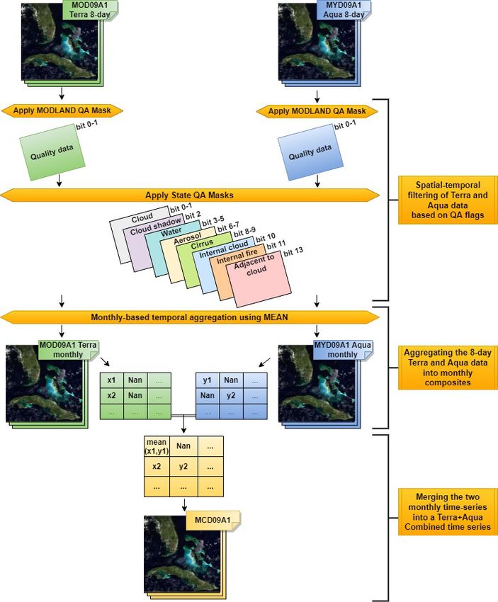
Table 2. Description of the GEE global LULC products used in this study.

                                              Product ID   Products           Version   Provider                  Sensor         Satellite or      Spatial res-   Acquisition   Data type           Link          Ref.
                                                                                                                                 spaceborne        olution        time
                                              P1:P5        MCD12Q1                v6    NASA LP DAAC              MODIS          Aqua–Terra        500 m          2001–2019     Image collection    MCD (2022)    Friedl and Sulla-Menashe (2019)
                                                           (LC type 1 to 5)             at the USGS
                                                                                                                                                                                                                                                    R. Khaldi et al.: TimeSpec4LULC

                                                                                        EROS Center
                                              P6           CGLS-               v3.0.1   Copernicus Global                        PROBA-V           100 m          2015–2019     Image collection    CGL (2022)    Buchhorn et al. (2020)
                                                           LULC100                      Land Service (CGLS)

https://doi.org/10.5194/essd-14-1377-2022
                                              P7           GFCC                   v3    NASA LP DAAC at           Multi-sensor   Multi-satellite   30 m           2000, 2005,   Image collection    GFC (2022a)   Sexton et al. (2013)
                                                                                        the USGS EROS                                                             2010, 2015
                                                                                        Center
                                              P8           GLOBCOVER              v2    ESA and by the Catholic   MERIS          ENVISAT           300 m          2009          Single      image   Glo (2022)    Arino et al. (2008)
                                                                                        University of Louvain
                                              P9           GFSAD                v0.1    Global Food Security      Multi-sensor   Multi-satellite   1000 m         2010          Single      image   GFS (2022)    Teluguntla et al. (2015)
                                                                                        support Analysis Data
                                                                                        at 30 m project
                                                                                        (GFSAD30)
                                              P10          PALSAR2               vfnf   JAXA EORC                 SAR            ALOS, ALOS2       25 m           2007–2010     Single      image   PAL (2022)    Shimada et al. (2014)
                                                                                                                                                                  2015–2017
                                              P11          HANSEN               v1.7    Hansen, UMD,              OLI            Landsat 8         30.92 m        2000–2019     Single      image   Han (2022)    Hansen et al. (2013)
                                                                                        Google, USGS, NASA
                                              P12          GFCH                v2005    NASA, JPL                                Lidar             927.67 m       2005          Single      image   GFC (2022b)   Simard et al. (2011)
                                              P13          JRC yearly           v1.2    EC JRC, Google            Multi-sensor   Landsat (5, 7,    30 m           1984–2019     Image collection    JRC (2022b)   Pekel et al. (2016)
                                                           water                                                                 8)
                                                           classification
                                                           history
                                              P14          JRC global           v1.2    EC JRC, Google            Multi-sensor   Landsat (5, 7,    30 m           1984–2019     Single      image   JRC (2022a)   Pekel et al. (2016)
                                                           surface                                                               8)
                                                           water mapping
                                                           layers
                                              P15          Tsinghua              v10    Tsinghua University       Multi-sensor   Landsat           30 m           1985–2018     Single      image   Tsi (2022)    Gong et al. (2020)
                                                           FROM-GLC

Earth Syst. Sci. Data, 14, 1377–1411, 2022
                                                                                                                                                                                                                                                    1381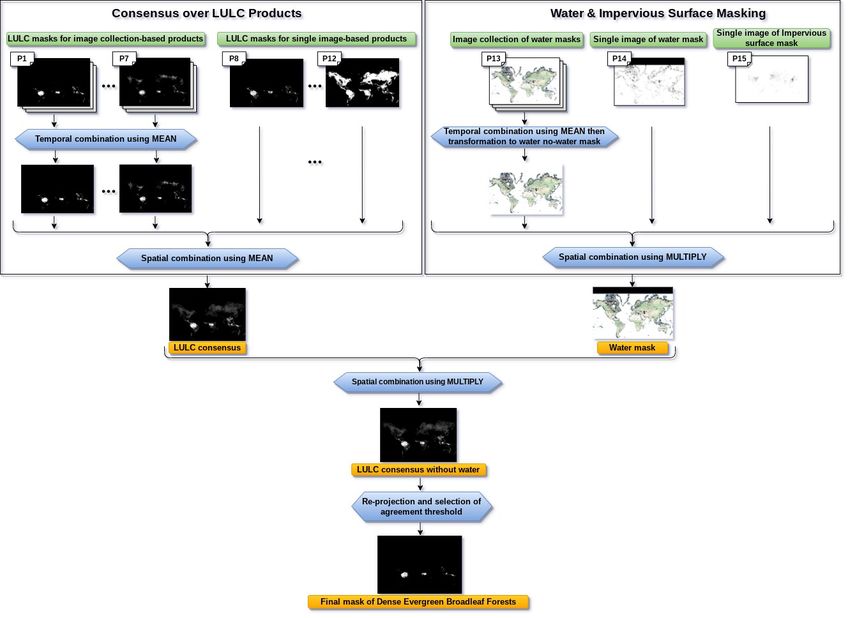
1382                                                                                                 R. Khaldi et al.: TimeSpec4LULC

Figure 1. Hierarchical structure of the LULC classes contained in the TimeSpec4LULC dataset. C1 to C29: the 29 LULC classes. L0 to L5:
the 5 LULC levels. L0 includes the 2 blue boxes. L1 includes the 4 green boxes. L2 includes the 12 yellow boxes. L3 includes all the classes
of the 12 yellow boxes (from C1 to C5 and from C18 to C29) except the forests class where it includes only the 2 orange boxes (deciduous
and evergreen). L4 includes the same classes but expands the forests class into the 4 purple boxes: deciduous (broadleaf and needleleaf) and
evergreen (broadleaf and needleleaf). L5 includes all the 29 LULC classes (from C1 to C29).

Table 3. Description of the full name and short name of each LULC       across the LULC products. Based on their data type, the
class in the TimeSpec4LULC dataset.                                     LULC products can be classified into two main categories:
                                                                        (1) products with single image referring to a particular year
  Class ID   Class full name                         Class short name   or period (P1 to P7) and (2) products with a collection of im-
  C1         Barren lands                            BarrenLands        ages over years (P8 to P12). Thus, the temporal agreement
  C2         Moss and lichen lands                   MossAndLichen      can only be applied for the second category of products. In
  C3         Grasslands                              Grasslands
  C4         Open shrublands                         ShrublandOpen
                                                                        (1) the single-image-based products, we obtained a binary
  C5         Closed shrublands                       ShrublandClosed    mask where value 1 corresponds to the targeted LULC class,
  C6         Open deciduous broadleaf forests        ForestsOpDeBr      whereas in (2) the image-collection-based products, we first
  C7         Closed deciduous broadleaf forests      ForestsClDeBr      obtained a binary mask for each year, and then we produced
  C8         Dense deciduous broadleaf forests       ForestsDeDeBr
  C9         Open deciduous needleleaf forests       ForestsOpDeNe
                                                                        their combination over years to obtain one mask. Afterwards,
  C10        Closed deciduous needleleaf forests     ForestsClDeNe      we performed a spatial agreement over the 12 masks of the
  C11        Dense deciduous needleleaf forests      ForestsDeDeNe      first 12 products (P1 to P12), and then we used the masks of
  C12        Open evergreen broadleaf forests        ForestsOpEvBr      the two water bodies products (P13 and P14) and the mask
  C13        Closed evergreen broadleaf forests      ForestsClEvBr
  C14        Dense evergreen broadleaf forests       ForestsDeEvBr
                                                                        of the impervious surface product (P15) to further refine the
  C15        Open evergreen needleleaf forests       ForestsOpEvNe      consensus.
  C16        Closed evergreen needleleaf forests     ForestsClEvNe         Based on the temporal consistency, the LULC classes
  C17        Dense evergreen needleleaf forests      ForestsDeEvNe      can be classified into (1) classes with high temporal stabil-
  C18        Mangrove wetlands                       WetlandMangro
  C19        Swamp wetlands                          WetlandSwamps
                                                                        ity, namely urban and built-up areas, water bodies, perma-
  C20        Marshland wetlands                      WetlandMarshl      nent snow, open shrublands, barren lands, and grasslands;
  C21        Marine water bodies                     WaterBodyMari      and (2) classes with low temporal stability characterized
  C22        Continental water bodies                WaterBodyCont      with plausible inter-annual changes, namely moss and lichen
  C23        Permanent snow                          PermanentSnow
  C24        Croplands flooded with seasonal water   CropSeasWater
                                                                        lands, forests, closed shrublands, wetlands, and croplands.
  C25        Irrigated cereal croplands              CropCereaIrri      This instability is due to several reasons, for example wet-
  C26        Rainfed cereal croplands                CropCereaRain      lands affected by droughts, or large areas of no-forest cover
  C27        Irrigated broadleaf croplands           CropBroadIrri      in one year preceded and followed by forest in the previ-
  C28        Rainfed broadleaf croplands             CropBroadRain
  C29        Urban and built-up areas                UrbanBlUpArea
                                                                        ous and following years, respectively. Our main objective is
                                                                        to collect from each class a representative number of pix-
                                                                        els that satisfy the temporal stability constraint of a specific
                                                                        class type. Thus, the temporal agreement, over the masks of

Earth Syst. Sci. Data, 14, 1377–1411, 2022                                                https://doi.org/10.5194/essd-14-1377-2022
R. Khaldi et al.: TimeSpec4LULC 1383
each image-collection-based product, was performed based
on two different types of operators governed by Algorithm 1.
(1) The AND operator, which represents a hard temporal sta-
bility constraint, ensures getting pixels with stable class type
over time but more likely a small number of pixels. (2) The
MEAN operator, which represents a soft temporal stability
constraint, provides a large number of pixels but with fewer
stability patterns over time. A list of these operators mapping
each LULC class is provided in Table 5.
Subsequently, the spatial combination of the 15 masks was
performed following six rules according to the global abun-
dance of each class. The main rule (Rule 1) is to apply the
MEAN operator across products P1 to P12 and multiply the
result by the two water masks of P13 and P14 to eliminate 2.1.4 Re-sampling and selection of agreement threshold
water pixels from land classes and land pixels from water
classes, as well as by the impervious surface mask of P15 to The final mask of each LULC class maintained the spa-
eliminate impervious pixels from all classes but urban. How- tial resolution of the last aggregated LULC product P15 at
ever, when the number of pixels for some LULC classes is 30 m resolution. The 30 m resolution LULC consensus was
small (less than 1000), Rule 1 was relaxed differently, gen- re-sampled with MODIS resolution (approximately equal to
erating five other different rules (Rule 2 to Rule 6). These 500 m) using the spatial MEAN reducer. This 500 m average
five rules were applied to five LULC classes that had too few consensus was used to explore different agreement thresh-
pixels with Rule 1: the moss and lichen lands (Rule 2), man- olds θ for each LULC class. We used θ = 1 when the number
grove wetlands (Rule 3), swamp wetlands (Rule 4), marsh- of retrieved 500 m pixels is greater than 1000, which means
land wetlands (Rule 5), and croplands flooded with seasonal that the 15 LULC products totally agree on the class type
water (Rule 6). The usage of the spatial combination rules is of these pixels. Otherwise, we decreased the threshold θ by
described in Algorithm 2. 0.05 until we reached at least 1000 pixels (Algorithm 3). Ta-
Finally, the spatial–temporal combination of the 15 LULC ble 7 provides the number of pixels obtained with each agree-
products resulted in a mask for each LULC class produced ment threshold. In any case, our dataset provides as metadata
at the resolution of the finest product (i.e., 30 m), where each the agreement percentage at pixel level, so that the user can
pixel had a consensus level value p in [0, 1]. Hence, for each control the desired agreement threshold and subsequent sam-
LULC mask, the pixel value p indicates the spatial–temporal ple size. To ensure collecting at least 1000 pixels from each
agreement degree over the 15 LULC products on the be- class, the lowest pixel-agreement threshold used is θ = 0.80
longing of this pixel to the class represented by this mask. (Table 7).
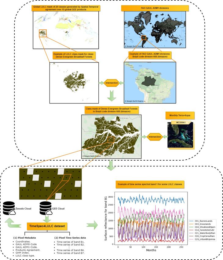
After performing, for each LULC class, the spatial–
temporal agreement, the re-projection, and the selection of
the agreement threshold, we combined the final class masks
of all the 29 LULC classes to generate one global LULC
map describing their distribution (Fig. 2). This figure shows
in which place of the world the 29 LULC classes are more
stable in time and the 15 LULC products are more compli-
ant, since the number of the collected pixels in each class is
affected by the temporal consistency of the 29 LULC classes
and the spatial consistency over the 15 LULC products. To
illustrate all the steps of the spatial–temporal agreement pro-
cess across the 15 global LULC products, we provide an
example explaining the generation of the final mask for the
class “dense evergreen broadleaf forests” (Fig. 3).
https://doi.org/10.5194/essd-14-1377-2022 Earth Syst. Sci. Data, 14, 1377–1411, 2022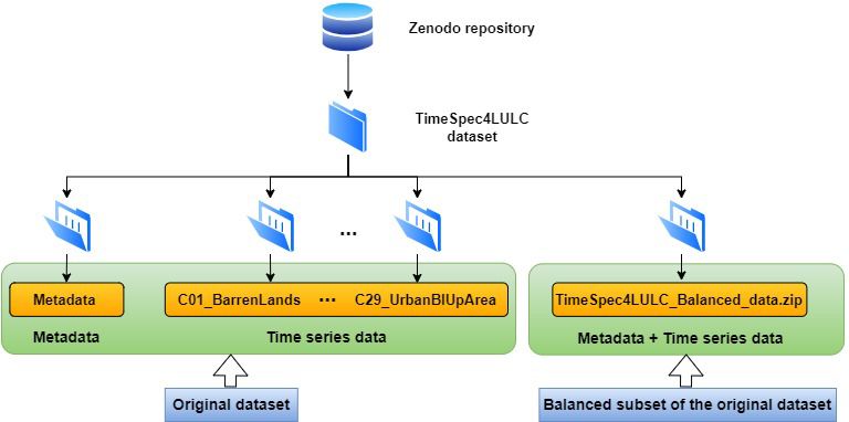
R. Khaldi et al.: TimeSpec4LULC
https://doi.org/10.5194/essd-14-1377-2022
Table 4. The rule set used to build the legend and define each LULC class in the TimeSpec4LULC dataset. P1 to P15: product 1 to 15. C1 to C29: class 1 to 29. The numbers from 0
to 220 correspond to class IDs in the original LULC products in Google Earth Engine. NU: not used; NA: not available; TC: tree cover; G: gain; L: loss; D: data mask; TH: tree height;
TCC: tree canopy cover; TCF: tree-cover fraction; SCF: shrub-cover fraction.
P1 P2 P3 P4 P5 P6 P7 P8 P9 P10 P11 P12 P13 P14 P15
C1 16 15 NA 7 11 60 TCC < 10 200 0 2 (TC < 10) ∩ (G = 0) ∩ (L = 0) ∩ (D 6 = 2) TH < 1 1∪0 0 Not (≥ 1)
C2 16 15 NA 7 11 100 TCC < 10 200 ∪ 150 0 2 (TC < 10) ∩ (G = 0) ∩ (L = 0) ∩ (D 6 = 2) TH < 1 1∪0 0 Not (≥ 1)
C3 10 10 1 6 6 30 TCC < 10 140 NA 2 (TC < 10) ∩ (G = 0) ∩ (L = 0) ∩ (D 6 = 2) TH < 2 1∪0 0 Not (≥ 1)
C4 7 7 2 NA 5 20 ∪ (10 < SCF < 50) TCC < 10 150 0 2 (TC < 10) ∩ (G = 0) ∩ (L = 0) ∩ (D 6 = 2) TH < 2 1∪0 0 Not (≥ 1)
C5 6 6 2 NA 5 20 ∪ (SCF > 50) TCC < 10 130 0 2 (TC < 10) ∩ (G = 0) ∩ (L = 0) ∩ (D 6 = 2) TH < 2 1∪0 0 Not (≥ 1)
C6 NA NA NA 4 4 4 + (15 < TCF < 30) 15 < TCC < 30 60 NA 1 (15 < TC < 30) ∩ (G = 0) ∩ (L = 0) ∩ (D 6 = 2) TH > 2 1∪0 0 Not (≥ 1)
C7 NA NA NA 4 4 4 + (40 < TCF < 60) 40 < TCC < 60 50 NA 1 (40 < TC < 60) ∩ (G = 0) ∩ (L = 0) ∩ (D 6 = 2) TH > 2 1∪0 0 Not (≥ 1)
C8 4 4 6 4 4 4 + (TCF > 60) TCC > 60 50 NA 1 (TC > 60) ∩ (G = 0) ∩ (L = 0) ∩ (D 6 = 2) TH > 2 1∪0 0 Not (≥ 1)
C9 NA NA NA 3 3 3 + (15 < TCF < 30) 15 < TCC < 30 NA NA 1 (15 < TC < 30) ∩ (G = 0) ∩ (L = 0) ∩ (D 6 = 2) TH > 2 1∪0 0 Not (≥ 1)
C10 NA NA NA 3 3 3 + (40 < TCF < 60) 40 < TCC < 60 NA NA 1 (40 < TC < 60) ∩ (G = 0) ∩ (L = 0) ∩ (D 6 = 2) TH > 2 1∪0 0 Not (≥ 1)
C11 3 3 8 3 3 3 + (TCF > 60) TCC > 60 NA NA 1 (TC > 60) ∩ (G = 0) ∩ (L = 0) ∩ (D 6 = 2) TH > 2 1∪0 0 Not (≥ 1)
C12 NA NA NA 2 2 2 + (15 < TCF < 30) 15 < TCC < 30 40 NA 1 (15 < TC < 30) ∩ (G = 0) ∩ (L = 0) ∩ (D 6 = 2) TH > 2 1∪0 0 Not (≥ 1)
C13 NA NA NA 2 2 2 + (40 < TCF < 60) 40 < TCC < 60 40 NA 1 (40 < TC < 60) ∩ (G = 0) ∩ (L = 0) ∩ (D 6 = 2) TH > 2 1∪0 0 Not (≥ 1)
C14 2 2 5 2 2 2 + (TCF > 60) TCC > 60 40 NA 1 (TC > 60) ∩ (G = 0) ∩ (L = 0) ∩ (D 6 = 2) TH > 2 1∪0 0 Not (≥ 1)
C15 9 9 NA 1 1 1 + (15 < TCF < 30) 15 < TCC < 30 90 NA 1 (15 < TC < 30) ∩ (G = 0) ∩ (L = 0) ∩ (D 6 = 2) TH > 2 1∪0 0 Not (≥ 1)
C16 8 8 4 1 1 1 + (40 < TCF < 60) 40 < TCC < 60 70 NA 1 (40 < TC < 60) ∩ (G = 0) ∩ (L = 0) ∩ (D 6 = 2) TH > 2 1∪0 0 Not (≥ 1)
C17 1 1 7 1 1 1 + (TCF > 60) TCC > 60 70 NA 1 (TC > 60) ∩ (G = 0) ∩ (L = 0) ∩ (D 6 = 2) TH > 2 1∪0 0 Not (≥ 1)
C18 11 11 NA NA NA 90 TCC > 10 170 NA NA (TC > 10) ∩ (G = 0) ∩ (L = 0) ∪ (D = 2) TH > 2 2∪3 1 Not (≥ 1)
a. 160 ∪ 180
C19 11 11 NA NA NA 90 TCC > 10 NA NA (TC > 10) ∩ (G = 0) ∩ (L = 0) ∪ (D = 2) TH > 2 2∪3 1 Not (≥ 1)
Earth Syst. Sci. Data, 14, 1377–1411, 2022
b. Not (170)
160 ∪ 170
C20 11 11 NA NA NA 90 TCC < 10 NA NA (TC < 10) ∩ (G = 0) ∩ (L = 0) ∪ (D = 2) TH < 2 2∪3 1 Not (≥ 1)
∪180
C21 17 0 0 0 0 200 NA 210 NA 3 NA NA 3 1 Not (≥ 1)
C22 17 0 0 0 0 80 NA 210 NA 3 NA NA 3 1 Not (≥ 1)
C23 15 NA NA NA 10 70 NA 220 NA NA NA NA 1∪0 0 Not (≥ 1)
1∪2∪3 0∪4∪5 Not (≥ 1)
C24 12 12 3∪1 5∪6 7∪8 40 NA 11 ∪ 14 NA NA NA 2∪3
∪4 ∪ 5 ∪8 ∪ 10
C25 12 12 1 6 7 40 NA 11 1∪2 NA NA NA 1∪0 0 Not (≥ 1)
C26 12 12 1 6 7 40 NA 14 3∪4∪5 NA NA NA 1∪0 0 Not (≥ 1)
C27 12 12 3 5 8 40 NA 11 1∪2 NA NA NA 1∪0 0 Not (≥ 1)
C28 12 12 3 5 8 40 NA 14 3∪4∪5 NA NA NA 1∪0 0 Not (≥ 1)
C29 13 13 10 8 9 50 NA 190 NA NA NA NA 1∪0 0 NU
1384
R. Khaldi et al.: TimeSpec4LULC                                                                                              1385

                                                                     2.2.2   Aggregating the original 8 d Terra and Aqua data
                                                                             into monthly composites
                                                                     Filtering the MODIS Terra and Aqua data records produced
                                                                     many missing values in their 8 d time series. To overcome
                                                                     this issue and further reduce the presence of noise in our
                                                                     dataset, the original 8 d time series were aggregated into
                                                                     monthly composites by computing the mean over the obser-
                                                                     vations of each month. Indeed, despite the fact that reduc-
                                                                     ing the temporal resolution from 8 d to monthly composites
                                                                     shortened the time series size, it generated two datasets with
                                                                     fewer missing values and clear monthly patterns, which are
2.2     Extracting times series of spectral data for 29 LULC         more intuitive to track LULC dynamics than the 8 d patterns.
        classes globally

To extract the 22-year monthly time series of the seven 500 m        2.2.3   Merging the two monthly time series into a
MODIS spectral bands for each of the 29 LULC classes                         Terra + Aqua combined time series
throughout the entire world, we followed four steps (Fig. 4):        Terra satellite daily orbits above the Earth’s surface from
(1) spatial–temporal filtering of Terra and Aqua data based          north to south in the morning at around 10:30 local time,
on quality assessment flags, (2) aggregation of the original         while Aqua orbits in the opposite direction in the after-
8 d Terra and Aqua data into monthly composites, (3) merg-           noon at around 13:30. Having two opportunities per day at
ing of the two monthly time series into a Terra + Aqua               each location increases the chances of capturing an image
combined time series, and (4) data extraction and archiving          under good atmospheric conditions. To further reduce the
(Fig. 6).                                                            number of missing values in our dataset, we merged the
                                                                     monthly time series provided by these two satellites into a
                                                                     Terra + Aqua combined time series. That is, for each pixel,
2.2.1    Spatial–temporal filtering of Terra and Aqua data           band, and month, when both Terra and Aqua had values,
         based on quality assessment flags                           we used the mean between them; when one satellite had a
                                                                     missing value, we used the available one; and when both of
MODIS sensor has high temporal coverage, ensured by Terra
                                                                     them had missing values, the combined value remains miss-
and Aqua satellite revisit frequencies, and also spectral and
                                                                     ing. Since Aqua was launched 3 years later (in 2002) after
spatial features that are highly suitable for LULC mapping
                                                                     Terra had been launched, the acquisition time of our dataset
and change detection (García-Mora et al., 2012; Xiong et al.,
                                                                     is (1) from 5 March 2000 to 4 July 2002 using Terra time
2017). Thus, we used two MODIS products, MOD09A1
                                                                     series and (2) from 4 July 2002 to 19 December 2021 using
(Ter, 2022) and MYD09A1 (Aqu, 2022), that estimate the 8 d
                                                                     Terra + Aqua time series.
surface spectral reflectance for the seven 500 m bands from
Terra and Aqua, respectively.
    The quality of any time series of satellite imagery is af-       2.2.4   Extracting and archiving the dataset
fected by the internal malfunction of satellite sensor at-           One of the main advantages of our dataset is its global-scale
mospheric (i.e., clouds, shadows, cirrus, etc.) or land (i.e.,       characteristic since all the LULC data were extracted glob-
floods, snow, fires, etc.) conditions. In addition to the spectral   ally from all the regions over the world. The data exporta-
bands, MODIS products provide quality assessment (QA)                tion process was performed in two steps (Fig. 6). (1) We ex-
flags as metadata bands to allow the user to filter out spec-        ported the metadata of all the pixels generated by the consen-
tral values affected by disruptive conditions. Therefore, all        sus. Then, (2) we exported their corresponding time series
QA flags were used to remove noise, spurious values, and             data. Detailed descriptions and discussions about each step
outliers in the image collection. MODLAND QA flags (bits             are provided as follows.
0–1) were used to only select pixel values produced at ideal
quality.                                                              1. From each LULC class mask, we first exported the
    Then, State QA flags were used to mask out clouds (bits 0–           metadata of all the available pixels in one file. However,
1), internal clouds (bit 10), pixels adjacent to clouds (bit 13),        for the class masks having more than 1 million pixels
cirrus (bits 8–9), cloud shadows (bit 2), high aerosol quan-             (barren lands, water bodies, permanent snow, grass-
tities (bits 6–7), and internal fires (bit 11). The water flag           lands, open shrublands, and dense evergreen broadleaf
(bits 3–5) was used to mask out water pixels in all terres-              forests) we only exported the metadata of 500 000 pix-
trial systems, but not in the terrestrial systems of permanent           els randomly selected over the globe because of the
snow, and in croplands flooded with seasonal water to avoid              memory limitations in GEE (Table 7). The exported
unrealistic data loss.                                                   metadata includes the coordinates of the pixel center

https://doi.org/10.5194/essd-14-1377-2022                                           Earth Syst. Sci. Data, 14, 1377–1411, 2022
1386                                                                                                                             R. Khaldi et al.: TimeSpec4LULC

Table 5. Description of the temporal–spatial combination of the 15 global LULC products (P1 : P15) masks to build a consensus image for
each LULC class.

   Class ID        LULC class(s)                                       Spatial combination                                                            Temporal
                                                                                                                                                      combination∗
   C1              Barren lands                                        Rule 1: mean(P1 : P12) · P13 · P14 · P15                                       Operator 1: AND
   C2              Moss and lichen lands                               Rule 2: mean(P1 : P5, P7 : P12) · P6 · P13 · P14 · P15                         Operator 2: MEAN
   C3              Grasslands                                          Rule 1: mean(P1 : P12) · P13 · P14 · P15                                       Operator 1: AND
   C4              Open shrublands                                     Rule 1: mean(P1 : P12) · P13 · P14 · P15                                       Operator 1: AND
   C5              Closed shrublands                                   Rule 1: mean(P1 : P12) · P13 · P14 · P15                                       Operator 2: MEAN
   C6:C17          Forests                                             Rule 1: mean(P1 : P12) · P13 · P14 · P15                                       Operator 2: MEAN
   C18             Mangrove wetlands                                   Rule 3: mean(P1 : P7, P9 : P14) · P8 · P15                                     Operator 2: MEAN
   C19             Swamp wetlands                                      Rule 4: mean(P1 : P8.a, P9 : P12) · P8.b · P15                                 Operator 2: MEAN
   C20             Marshland wetlands                                  Rule 5: mean(P1 : P6, P8 : P10, P13 : P14) · P7 · P11 · P12 · P15              Operator 2: MEAN
   C21:C22         Water bodies                                        Rule 1: mean(P1 : P12) · P13 · P14 · P15                                       Operator 1: AND
   C23             Permanent snow                                      Rule 1: mean(P1 : P12) · P13 · P14 · P15                                       Operator 1: AND
   C24             Croplands flooded with seasonal water               Rule 6: mean(P1 : P12) · (P13 OR P14) · P15                                    Operator 1: AND
   C25 : C26       Cereal croplands                                    Rule 1: mean(P1 : P12) · P13 · P14 · P15                                       Operator 1: AND
   C27 : C28       Broadleaf croplands                                 Rule 1: mean(P1 : P12) · P13 · P14 · P15                                       Operator 1: AND
   C29             Urban and built-up areas                            Rule 1: mean(P1 : P12) · P13 · P14 · P15                                       Operator 1: AND
∗ Inter-annual combination used in all products except in P13, where we first calculated the inter-annual mean and then transformed it into a water–no-water binary mask.

Figure 2. Distribution of the number of covered countries (Food and Agricultural Organization’s Global Administrative Unit Layers 2015
GAUL-ADM0) over the 29 LULC classes. This map combines all the final LULC class masks that were generated from the process of
spatial–temporal agreement across the 15 global LULC products available in GEE. In the map’s legend we are presenting the short names of
the LULC classes (their corresponding full names are presented in Table 3).

Earth Syst. Sci. Data, 14, 1377–1411, 2022                                                                         https://doi.org/10.5194/essd-14-1377-2022
R. Khaldi et al.: TimeSpec4LULC 1387
Figure 3. Example of the final mask creation process for the dense evergreen broadleaf forests LULC class produced through the spatial–
temporal agreement over the 15 global LULC products available in GEE.
and the percentage of agreement over the 15 LULC of human modification of terrestrial lands. Then, it was
products. To take into account all the differences across projected to MODIS resolution using the spatial mean
the globe and thinking of regional interests that some reducer to generate the average GHM index.
users may have, we used the Food and Agricultural
2. After exporting the metadata, we accessed the coordi-
Organization’s Global Administrative Unit Layers 2015
nates of each LULC class to download their time se-
(FAO GAUL) product, available in GEE, to provide
ries data for the seven spectral bands (Table 6). Each
for each pixel the ADM0-CODE obtained from the
time series dataset contains 262 observations covering
country boundaries (GAU, 2022a) of FAO GAUL (i.e.,
almost 22 years (i.e., from 2000 to the end of 2021).
countries) and the ADM1-CODE obtained from the
In order to optimize the exportation process, for each
first-level administrative units (GAU, 2022b) of FAO
LULC class, the 262 observations corresponding to the
GAUL (e.g., departments, states, provinces). Further,
262 months were exported separately in 262 parallel re-
to provide the user with extra metadata that could be
quests. In each request, we exported seven values corre-
used to filter time series according to different levels
sponding to the seven spectral bands for all the LULC-
of human intervention on each pixel, the average GHM
class-related pixels.
index was included. The GHM index was derived from
the Global Human Modification dataset (CSP gHM) The exported data generated highly imbalanced LULC
(https://developers.google.com/earth-engine/datasets/ classes obviously due to the differences in their spatial dis-
catalog/CSP_HM_GlobalHumanModification?hl=en, tributions. Thus, to facilitate the exploration of the dataset,
last access: 22 March 2022; Kennedy et al., 2019) we also provided a balanced dataset ready to train machine
available in GEE, which provides a cumulative measure learning models. The balanced subset of TimeSpec4LULC
provides the time series data for 1000 pixels from each class
https://doi.org/10.5194/essd-14-1377-2022 Earth Syst. Sci. Data, 14, 1377–1411, 20221388 R. Khaldi et al.: TimeSpec4LULC Figure 4. Description of the spatial–temporal filtering of Terra and Aqua, their aggregation into monthly composites, and their merging into Terra + Aqua combined time series. This process aims to filter out spectral values affected by disruptive conditions and to reduce the number of gaps in the multispectral time series for the 29 LULC classes. since the smallest LULC class contains 1194 pixels (Ta- Then, the user can upload these coordinates to GEE to export ble 7). The selection of these 1000 samples from each class the time series data of the desired range of time. was performed using Algorithm 4 such that they are evenly distributed in the globe and representative for the world. In Fig. 5, we provide the distribution of the 1000 pixels selected from the class “marine water bodies”. The provided metadata can also be used in case the user wants to export future time series observations for the com- ing months. In this context, the user needs to make use of the ADM0-CODE and the ADM1-CODE to access the coor- dinates of any region in the world included in the consensus. Earth Syst. Sci. Data, 14, 1377–1411, 2022 https://doi.org/10.5194/essd-14-1377-2022
R. Khaldi et al.: TimeSpec4LULC                                                                                               1389

Table 6. Description of the seven spectral bands of MODIS sensor.

                             Band ID    Band name          Wavelength      Description
                             B1         MCD09A1_B1         620–670 nm      Surface reflectance for band 1
                             B2         MCD09A1_B2         841–876 nm      Surface reflectance for band 2
                             B3         MCD09A1_B3         459–479 nm      Surface reflectance for band 3
                             B4         MCD09A1_B4         545–565 nm      Surface reflectance for band 4
                             B5         MCD09A1_B5         1230–1250 nm    Surface reflectance for band 5
                             B6         MCD09A1_B6         1628–1652 nm    Surface reflectance for band 6
                             B7         MCD09A1_B7         2105–2155 nm    Surface reflectance for band 7

                                                                          The remaining 29 folders contain the time series data for
                                                                          the 29 LULC classes. Each folder has the form “Clas-
                                                                          sId_ClassShortName” and holds 262 CSV files corre-
                                                                          sponding to the 262 months. For example, the CSV file
                                                                          for the barren lands class for the last month is named
                                                                          “C01_261.csv”. Inside each CSV file, we provide the
                                                                          seven values of the spectral bands as well as the coordi-
                                                                          nates for all the LULC-class-related pixels.
                                                                          A clear description of the metadata folder along with
                                                                          an example of the time series data for barren lands is
                                                                          presented in Fig. 8.

                                                                        – The balanced subset of the original dataset holds the
                                                                          metadata and the time series data for 1000 pixels per
                                                                          class representative of the globe selected by Algo-
3     Data                                                                rithm 4. It contains 29 different JSON files following the
                                                                          names of the 29 LULC classes. The naming of each file
To organize and assess the quality of the extracted global data           follows the structure “ClassId_ClassShortName.json”.
for all the 29 LULC classes, we first present the description             For instance, the JSON file for the barren lands class
of the dataset structure, and then we evaluate the quality of             is named “C01_BarrenLands.json”.
its annotation process.
                                                                          Each JSON file “Class_File” is a dictionary containing
                                                                          the short name of the LULC class “Class_Name”, the
3.1    Description of the data structure                                  ID of the class “Class_Id”, and a list of all the relative
                                                                          pixels “Pixels” (for more information about the LULC
The      TimeSpec4LULC        dataset     is   hosted     by              classes short names, see Table 3). Each element of the
https://doi.org/10.5281/zenodo.5020024 (Khaldi et al.,                    list “Pixels” is a dictionary holding the ID of the pixel
2022). It contains two datasets: the original dataset “Time-              “Pixel_Id”, the class of the pixel “Pixel_Label”, the
Spec4LULC_Original_data.zip” and the balanced subset of                   metadata of the pixel “Pixel_Metadata”, and the seven
the original dataset “TimeSpec4LULC_Balanced_data.zip”.                   time series of the pixel “Pixel_TS”.
The structure of TimeSpec4LULC is organized as follows
(Fig. 7).                                                                 The variable “Pixel_Metadata” contains the geometry
                                                                          and coordinates (longitude and latitude) of the pixel
    – The original dataset contains 30 folders, namely “Meta-             center following the GEE format “.geo”, the GAUL
      data”, and 29 folder corresponding to the 29 LULC                   country code “ADM0_Code”, the GAUL first-level ad-
      classes. The folder “Metadata” holds 29 different                   ministrative unit code “ADM1_Code”, the average of
      CSV files named on behalf of the 29 LULC classes.                   the global human modification index “GHM_Index”,
      The naming of each file follows the structure “Clas-                the agreement percentage over the 15 LULC prod-
      sId_metadata.csv”. For instance, the metadata CSV file              ucts “Products_Agreement_Percentage”, and a dictio-
      for the barren lands class is named “C01_metadata.csv”.             nary carrying the temporal availability percentage for
      Each CSV file holds the metadata of all the pixels gen-             each band “Temporal_Availability_Percentage” (i.e.,
      erated by the consensus limited to 500 000 for classes              percentage of non-missing data per band from B1 to
      that exceed 1 million at agreement threshold 1.                     B7).

https://doi.org/10.5194/essd-14-1377-2022                                           Earth Syst. Sci. Data, 14, 1377–1411, 2022
1390 R. Khaldi et al.: TimeSpec4LULC
Figure 5. Distribution of the 1000 points selected by Algorithm 4 for the class “marine water bodies”: (a) global view and (b) zoomed-in
view.
The variable “Pixel_TS” is a dictionary that holds the over the globe were selected. Figure 10 shows the dis-
names and the time series values of the seven spectral tribution of the 2900 selected pixels.
bands (from MCD09A1_B1 to MCD09A1_B7) of size
– Second, the class of each pixel of the 29 × 100 sam-
262. A clear description of the JSON class file is pre-
ples is identified visually by the expert eye following
sented in Fig. 9.
the next rule. We consider as ground truth the dominant
LULC class; such LULC class occupies at least 70 %
of the pixel. The presence of up to 30 % of features of
3.2 Data quality control other different LULC classes within the dominate class
The quality of the dataset annotation was assessed and is ignored.
validated visually by two co-author experts using two – Once the validated LULC classification matrix was ob-
very high resolution imagery (< 1 m/pixel) sources, namely tained (Table 8), the F1 score was calculated for all the
Google Earth (https://earth.google.com/web/, last access: LULC levels (from L0 to L5). We used F1 score because
22 March 2022) and Bing Maps imagery (https://www.bing. it evaluates the balance between precision and recall,
com/maps/, last access: 22 March 2022). The assessment where (1) precision indicates how accurate the annota-
process includes three stages. tion process is in predicting true positives and (2) the
recall, also called sensitivity, indicates how many actual
– First, a set of 100 samples is carefully selected from
positives were predicted as true positives (Eq. 3).
each class following the maximum distance criteria de-
scribed in Algorithm 4. That is, depending on the overall Precision × Recall
size of each LULC class, 100 evenly distributed pixels F1 score = 2 × (1)
Precision + Recall
Earth Syst. Sci. Data, 14, 1377–1411, 2022 https://doi.org/10.5194/essd-14-1377-2022R. Khaldi et al.: TimeSpec4LULC 1391 Figure 6. Description of the data extraction process for the LULC class dense evergreen broadleaf forests from all the world’s partitions (GAUL-ADM0, https://developers.google.com/earth-engine/datasets/catalog/FAO_GAUL_2015_level0, last access: 22 March 2022; and GAUL-ADM1, https://developers.google.com/earth-engine/datasets/catalog/FAO_GAUL_2015_level1, last access: 22 March 2022) where this class is available, in addition to a visualization of the first spectral band time series for some LULC classes. https://doi.org/10.5194/essd-14-1377-2022 Earth Syst. Sci. Data, 14, 1377–1411, 2022
1392                                                                                                 R. Khaldi et al.: TimeSpec4LULC

Table 7. Sensitivity analysis of the number of pixels with respect to different values of agreement thresholds along with the final number
of collected pixels at the selected threshold. When the number of pixels at threshold 1 exceeds 1 million, we collect 500 000 random pixels.
Otherwise, we decrease the threshold by 0.05 until we obtain at least 1000 pixels (Algorithm 3).

        Class    Class short name                           Agreement thresholds                            Collected     Selected
        ID                                  0.80          0.85          0.90           0.95             1       pixels   threshold
        C1       BarrenLands          85 293 945    83 484 114     81 157 460   73 495 569    65 332 858      500 000            1
        C2       MossAndLichen           646 305       482 619        287 757      134 549         2807         2807             1
        C3       Grasslands           55 588 334    34 749 935     21 729 176    4 082 093     1 032 092      500 000            1
        C4       ShrublandOpen        32 024 725    21 664 056     14 594 193    2 117 778       223 062      223 062            1
        C5       ShrublandClosed         549 792       128 113         38 656        2985              9        2985          0.95
        C6       ForestsOpDeBr           130 123         7034               4            0             0        7034          0.85
        C7       ForestsClDeBr           486 196        41 869            494            0             0       41 869         0.85
        C8       ForestsDeDeBr         6 646 105     4 765 433      2 993 393      387 276         2240         2240             1
        C9       ForestsOpDeNe             1402             28              0            0             0        1402          0.80
        C10      ForestsClDeNe            71 446         1348               0            0             0        1348          0.85
        C11      ForestsDeDeNe         1 109 793       703 062        242 614       10 979             0       10 979         0.95
        C12      ForestsOpEvBr             2719             86              0            0             0        2719          0.80
        C13      ForestsClEvBr            58 552         3322             149            1             0        3322          0.85
        C14      ForestsDeEvBr        49 150 065    45 678 189     40 445 318   32 048 990     3 000 060      500 000            1
        C15      ForestsOpEvNe             2735             10              0            0             0        2735          0.80
        C16      ForestsClEvNe           154 341         4332              26            0             0        4332          0.85
        C17      ForestsDeEvNe         6 987 918     4 562 614      1 966 655      558 406           362      558 406         0.95
        C18      WetlandMangro            14 095         4750             716           78             0        4750          0.85
        C19      WetlandSwamps             8453          1194             100            7             0        1194          0.85
        C20      WetlandMarshl            18 748         9491           4500         1405             80        1405          0.95
        C21      WaterBodyMari        47 953 196    46 869 483     40 323 857   39 200 046    35 848 199      500 000            1
        C22      WaterBodyCont        47 541 101    45 792 728      6 016 114    5 630 082     4 789 580      500 000            1
        C23      PermanentSnow         7 593 382     7 540 486      7 469 482    7 354 210     6 827 318      500 000            1
        C24      CropSeasWater           233 404       190 947        134 486       97 732        38 642       38 642            1
        C25      CropCereaIrri         6 559 822     4 949 682      1 392 245    1 005 469       405 340      405 340            1
        C26      CropCereaRain        17 025 686    13 632 125      6 334 106    3 693 354       848 583      848 583            1
        C27      CropBroadIrri         2 977 417     2 349 114      1 099 282      896 775       392 630      392 630            1
        C28      CropBroadRain         6 965 150     5 686 144      2 596 559    1 561 992       359 674      359 674            1
        C29      UrbanBlUpArea         1 832 276     1 178 905        704 481      501 219       159 073      159 073            1
        Total number of collected pixels                                                                    6 076 531

                    True Positive
Precision =                                                      (2)    4   Results and discussions
            True Positive + False Positive
                 True Positive                                          The total number of collected time series (pixels) in all the 29
Recall =                                                         (3)
         True Positive + False Negative                                 LULC classes is 6 076 531, which is large enough to build
                                                                        high-quality DL models (Table 7). This number covers the
As it can be observed from Table 8, as we go up from level              29 LULC classes in unbalanced way due to two reasons:
L0 to level L5 the obtained F1 score decreases from 96 % to             (1) the global abundance of each class and (2) the choice of
87 % mainly due to the classification of forests, grasslands,           the agreement threshold. We provide, in Table 7, the varia-
open shrublands, water bodies, and croplands flooded with               tion of the number of pixels with respect to different values
seasonal water. Typically, the obtained F1 score of each class          of agreement thresholds. It can be noticed that as we decrease
is independent of the selected agreement threshold. In some             the agreement threshold, the number of pixels increases. Ta-
classes, even if the agreement threshold is equal to 1, the F1          ble 7 highlights also the classes that reduced the consen-
score is low compared to other classes with small agreement             sus F1 score (with selected threshold less than 1) which are
threshold. For instance, the agreement threshold of grass-              the three wetlands classes, closed shrublands, and all forests
lands and open deciduous needleleaf forests is equal to 1               classes except dense deciduous broadleaf and dense ever-
and 0.80, respectively. However, the F1 score of grasslands is          green broadleaf.
lower (0.68) than the F1 score of open deciduous needleleaf                In 15 LULC classes, the number of collected time series, at
forests (0.90).                                                         agreement threshold 1, is at least 2240 per class. This means

Earth Syst. Sci. Data, 14, 1377–1411, 2022                                                https://doi.org/10.5194/essd-14-1377-2022
R. Khaldi et al.: TimeSpec4LULC 1393 Figure 7. Dataset structure. Figure 8. Data structure of the metadata folder (a) and the time series data folder (b) for the class “barren lands” in the original dataset. that the 15 LULC products are 100 % compliant with re- age temporal availability percentage is very high (e.g., grass- gard to the nature of these classes. Thus, these classes have lands, shrublands, and open deciduous broadleaf forests). enough pure spectral information, describing their behavior However, it is low for other classes (e.g., moss and lichen over time, to train DL models with very high accuracy. How- lands, marshland wetlands, marine water bodies, and perma- ever, in the remaining 14 LULC classes, the number of time nent snow), which implies that their multispectral time series series, collected at agreement threshold 100 %, is either small information is hugely affected by atmospheric and/or land (with closed shrublands, dense evergreen needleleaf forests, conditions. For all LULC classes, it is noticeable that the av- and marshland wetlands) or null in the remaining wetlands erage temporal availability percentage in band 6 is low com- classes and forests classes (except dense broadleaf classes). pared to the other bands which make band 6 the most con- This implies that, within 500 m pixels, the LULC products taminated by gaps. The reason behind this is the “dead lines” are less consistent within these classes, and there may be in Aqua band 6 caused by the already reported malfunction- remaining noise in one class from other classes. Since our ing or noise in some of its detectors (Zhang et al., 2018b). dataset provides, as metadata, the agreement percentage at The unbalanced dataset (Table 9) and the balanced dataset the pixel level, the user can always select the desired agree- corresponding to the 1000 pixels per class (Table 10) are dis- ment threshold. tributed all over the world’s GAUL partitions: ADM0 (i.e., The collected time series data in each LULC class still countries) and ADM1 (e.g., departments, states, provinces). contains some missing data that could be handled neither Each LULC class, in the two datasets, covers more than 6 with the monthly aggregation process nor with the Terra– countries and more than 13 departments, except moss and Aqua merging process (Table 10). For some classes, the aver- lichen lands as well as deciduous needleleaf forests that https://doi.org/10.5194/essd-14-1377-2022 Earth Syst. Sci. Data, 14, 1377–1411, 2022
You can also read