Towards a modular end-to-end statistical production process with mobile network data
←
→
Page content transcription
If your browser does not render page correctly, please read the page content below
S PANISH J OURNAL OF S TATISTICS
Vol. 2 No. 1 2020, Pages 41–77
doi:https://doi.org/10.37830/SJS.2020.1.04

R EGULAR A RTICLE

          Towards a modular end-to-end statistical
        production process with mobile network data
 David Salgado1, 2 , Luis Sanguiao1 , Bogdan Oancea3, 4 , Sandra Barragán1 , Marian Necula3
    1 Department      of Methodology and Development of Statistical Production, Statistics Spain (INE), Spain
         2 Department     of Statistics and Operations Research, Complutense University of Madrid, Spain
                 3 Department of Innovative Tools in Statistics, Statistics Romania (INS), Romania
                    4 Department of Business Administration, University of Bucharest, Romania

                                   Received: November 3, 2020. Accepted: March 1, 2021.

Abstract: Mobile network data has proved to be an outstanding data source for the production of
statistics in general, and for Official Statistics, in particular. Similarly to another new digital data
sources, this poses the remarkable challenge of refurbishing a new statistical production process.
In the context of the European Statistical System (ESS), we substantiate the so-called ESS Reference
Methodological Framework for Mobile Network Data with a first modular and evolvable proposed
statistical process comprising (i) the geolocation of mobile devices, (ii) the deduplication of mobile
devices, (iii) the statistical filtering to identify the target population, (iv) the aggregation into terri-
torial units, and (v) the inference to the target population. The proposal is illustrated with synthetic
data generated from a network event data simulator developed for these purposes.

Keywords: Statistical production, mobile network data, end-to-end process, geolocation, Dedupli-
cation, aggregation, inference

MSC: 62-07, 62P25, 62M05, 62F15

1     Introduction
Mobile network data, i.e. digital data generated in a mobile telecommunication network by the
interaction between a mobile station (mobile device such as a smartphone or a tablet) and a
base transceiver station (commonly known as antenna in an imprecise way) (Miao et al., 2016),
constitutes a remarkable source of information for the production of statistics in Social Science, in
general, and for Official Statistics, in particular. Many one-off studies can already be found in the
literature with applications in different statistical domains (González et al., 2008; Ahas et al., 2010;
Phithakkitnukoon et al., 2012; Calabrese et al., 2013; Deville et al., 2014; Louail et al., 2014; Iqbal
et al., 2014; Blondel et al., 2015; Douglass et al., 2015; Pappalardo et al., 2016; Raun et al., 2016;
Ricciato et al., 2017; Graells-Garrido et al., 2018; Wang et al., 2018) (see Salgado et al. (2020) for a
more comprehensive list).

© ine                                                       Published by the Spanish National Statistical Institute
42                                                                                        D. S ALGADO ET AL .

    However, the production of official statistics in National and International Statistical Systems
requests a standardized and industrialised statistical production process so that this new data source
is fully integrated in the daily production framework of statistical offices. This raises remarkable
challenges such as the data access conditions, new methodological and quality frameworks, a larger
IT infrastructure (both in hardware and in software), a deep revision of the statistical disclosure
control, and the identification of relevant aggregates (mostly included as part of legal regulations)
for a diversity of stakeholders and users. Although a number of illustrative case studies dealing with
official statistics can already be found in the literature (Debusschere et al., 2016; Williams, 2016;
Nurmi, 2016; Izquierdo-Valverde et al., 2016; Dattilo et al., 2016; Senaeve and Demunter, 2016;
Meersman et al., 2016; Reis et al., 2017; Sakarovitch et al., 2019; Galiana et al., 2018; Lestari et al.,
2018), we still lack a production framework with a new statistical process.

    In this line of thought, efforts in the international community (UN, 2017) and in the Europen
Statistical System (ESS) (Ricciato, 2018) are under way to construct a production framework and
some recent examples of an end-to-end statistical production process have been tested in a statistical
office (Tennekes et al., 2020). The need for a detailed standardised and harmonised statistical
process goes beyond the rise of new digital data sources, since a process-oriented production system
instead of a product-oriented or even domain-oriented system is nowadays considered essential to
achieve high-quality standards (UNECE, 2011). In this sense, the proliferation of one-off studies
with new digital data in different statistical domains may be stressing the risk over statistical offices
of reinforcing production silos, thus becoming clearly inefficient and making Official Statistics
socially irrelevant (DGINS, 2018).

    This article presents the fundamentals of a modular and evolvable statistical process with mobile
network data to produce estimates for present population counts and origin-destination matrices
as a concrete business case. This proposal constitutes the first step towards the construction
of the so-called ESS Reference Methodological Framework for Mobile Network Data (see e.g.
Ricciato, 2018), an initiative of the ESS embracing a set of principles to ensure consistency,
reproducibilty, portability, and evolvability of data processing methods for this data source, to
facilitate interworking between statistical offices and mobile network operators (MNOs) both at
technical and organisational levels, and to adapt to the fast-changing technological environment of
telecommunications by clearly detaching technology and statistical analysis.

    We shall focus on the integral view of the process underlying its functional modularity and evolv-
ability and on the methodological core bringing novel methods in Official Statistics with a clear goal
of producing both estimates and their quality indicators (accuracy). We shall illustrate the whole
process using synthetic network event data generated by a data simulator developed for these pur-
poses. In section 2 we provide a general description of our approach setting up the general context
under which this proposal is thought to be implemented. In section 3 we shall shortly describe the
main functionalities of the network event data simulator as of this writing. In section 4 we provide
the main contents of each of the modules comprising the statistical process, namely a generic de-
scription of the data in subsection 4.1, geolocation of mobile devices in subsection 4.2, deduplication
of mobile devices carried by the same individual in subsection 4.3, statistical filtering of individuals
in the target population in subsection 4.4, aggregation of device-level data into territorial units in
subsection 4.5, and inference with respect to the target population in subsection 4.6. In section 5 we
close with some conclusions and future prospects.
E ND - TO - END STATISTICAL PROCESS WITH MOBILE NETWORK DATA                                                                   43

2     General description
The development, implementation, and monitoring of a statistical production process with mobile
network data entail several complex and highly entangled issues. We need to solve questions
regarding the access to data (including the integration with other data sources and even data from
several MNOs), the development of statistical methods not traditional used in the production of
official statistics, the according update and modernisation of the quality assurance framework, the
deployment of the corresponding IT infrastructure, the professional and technical skills of staff
necessary to execute this process, and the identification of the key target aggregates to be produced
for the public good.

    Official statistics play a key role in democratic socities for decision-taking and policy-making.
For example, public fund allocation is usually conducted taking into account official population
figures published by statistical offices. Thus, high-quality standards must be ensured and verified
usually following international frameworks. In this context, in agreement with the ESS Reference
Methodological Framework, an official statistical process with mobile network data must comprise
the process design from the raw telecommunication data generated in the networks to the final
statistical outputs. Acquiring aggregates or data at device-level from unknown preprocessing
steps is not considered an option here. This is the first assumption motivating our proposal of an
end-to-end process.

   Mobile network data are extremely sensitive data and rightful concerns immediately arise to use
them for statistical purposes. Data access is indeed an intricately complex set of legal, administrative,
technical, and business issues, which we shall not dealt with here. Nonetheless, we assume three
principles around which a final solution must be built:
     • Privacy and confidentiality: as with any other official statistics produced from any data source
       by any statistical office, privacy and confidentiality of data holders and respondents must be
       assured. Indeed, stringent legal conditions have recently arisen to prevent privacy and confi-
       dentiality in the European context (European Parliament, 2016).
     • Public good: there is an evident socioeconomic interest in extracting different insights from
       mobile network data valuable for the public good. This is as legitimate as the production of
       official statistics from traditional data sources.
     • Private business interest: the production of statistical outputs and insights from mobile net-
       work data stands also as an increasing economic activity providing value and progress to the
       economy. Indeed, the digital data economy is targeted as a pillar in the European context.
    All in all, an aligment of these three principles must be reached in practice. The proposed
statistical process herein assumes that a collaborating scenario between statistical offices and MNOs
through public-private partnerships, joint ventures, etc. is possible and leaves room for the design,
execution, and monitoring of the different modules explained below.

    In the context of the ESS, as of this writing no definitive agreement for a fully-fledged sustainable
production of official statistics based on mobile network data has been reached between a national
statistical office (NSO) and an MNO. Only specific short-term limited agreements for research have
been reached1 . This entails a shortage of data in NSOs to develop the statistical methodology,
    1 A remarkable exception is the compilation of international travel statistics for the balance of payments produced by
the National Bank of Estonia (National Estonian Bank, 2020), not a statistical office, though.

                                                                                         SJS, VOL . 2, N O . 1 (2020), PP. 41 - 77
44 D. S ALGADO ET AL .
the quality frameworks, and the software tools. Furthermore, given the extraordinarily rich and
complex data ecosystem associated to a mobile telecommunication network, the identification of
concrete data for statistical purposes must be undertaken (Radio network data? Core network data?
Network management data? Call Detail Records?). In this sense, our strategy is to produce synthetic
network event data together with a ground truth scenario so that all these aspects can be developed
and investigated. In this way, more specific data requests can be formulated in agreement with the
quality indicators and the ground truth computed in the simulated scenarios. Thus, our starting
point will be the generation of these simulated scenarios.
A key feature of the ESS Reference Methodological Framework is the evolvability of the sta-
tistical process so that improvements and adaptations of the statistical methods to the underlying
technological conditions is always possible and seamless. This justifies the approach of functional
modularity (already present in modern proposals of traditional statistical processes (see e.g. Salgado
et al., 2018)). By breaking the end-to-end process into modules according to the data abstraction
principle we design transparent and independent production steps so that a change in one module
will not affect the next module beyond the quality of the input/output interconnecting them through
a standardised interface. In this proposal we do not include all necessary modules (e.g. data acquisi-
tion, substituted by the simulator) but only those core methodological stages (see Radini et al., 2020,
for an architectural point of view):
• Geolocation.- This module focuses on the computation of location probabilities for each device
across a reference grid used for the statistical analysis.
• Deduplication.- This module focuses on the computation of multiplicity probabilities for each
device, i.e. probabilities of a given device to be carried by an individual jointly with one or
several other devices. This is motivated by our interest on individuals of the target population,
not on mobile devices.
• Statistical filtering.- This module focuses on the algorithmic identification of mobile devices of
individuals of the target population such as domestic tourists, commuters, inbound tourists,
etc.
• Aggregation.- This module focuses on the computation of probability distributions for the
number of individuals detected by the network (i.e. with mobile devices) across different terri-
torial units.
• Inference.- This module focuses on the computation of probability distributions for the number
of individuals of the target population (even with no device) across different territorial units.
A cautious reader will immediately notice how the computation of probabilities is essential across
the whole process. The use of probabilities, in our view, is jointly motivated by several relevant
reasons. Firstly, probability distributions allow us to account for the uncertainty along the whole
process, thus paving the way for the computation of quality indicators, especially those related to ac-
curacy. Secondly, probability models provide a natural way to integrate data through priors and pos-
teriors in a hierarchy of models. This is important because the combination of diverse data sources
will not only produce statistical outputs with higher quality but it is also necessary in many cases,
in particular, with mobile network data to avoid identifiability problems (see below). Thirdly, prob-
ability distributions stand as a flexible module interface between the successive production steps. In
this line, we can use the total probability theorem to connect the original input data (raw telco data)
with the final output data (population estimates):E ND - TO - END STATISTICAL PROCESS WITH MOBILE NETWORK DATA 45
Physical Logical
Population counts, data flow data flow
origin-destination matrices
- Number of individuals
per territorial unit detected
in the network;
- Penetration rates;
- Register based population.
Inference layer
- Number of individuals
per territorial unit detected
in the network
Aggregation layer
- Device multiplicity probabilities;
- Territorial units (regions, …).
Secondary storage
- Device multiplicity probabilities
Deduplication layer
- Location probabilities
- Location probabilities
Geolocation layer
- Network event data;
- Network config parameters
(RSS, SDM, …)
- Aux info (land use, transport
networks, …)
Data acquisition and preprocessing layer
- Raw data (network event data,
other network config parameters)
The data acquisition interface
The core network
Figure 1: Modular structure of the statistical process and its software tools.
Z Z Z
P (zout |zin ) = dz1 dz2 · · · dzN P(zout |zN ) · · · P(z2 |z1 )P(z1 |zin ). (1)
The modular structure of the methodology is translated into a modular structure for the software
tools. The choice of programming languages to develop these tools is motivated by multiple reasons.
Firstly, software developed with the intention to be used in the future should be portable at the
level of source code. Thus, portability is our first consideration. Secondly, our goal is to produce a
software for statisticians, not for computer scientists. Thus, the language(s) of the implementation
should be familiar for statisticians and easy to use by them. Thirdly, in the line of software
development in the ESS, we planned to use only open source tools like libraries, IDEs, debuggers,
profilers, etc. to maintain the software development process under a strict control regarding the
associated costs. Moreover, the programming language(s) together with these tools should have a
large community of programmers and users which can be seen as a free technical support. Fourthly,
the programming language(s) should have support for parallel and distributed computing. Since all
the algorithms involved by the our methodological approach are computational intensive, and the
size of mobile network data could be very large, this is a mandatory requirement. Last but not least
SJS, VOL . 2, N O . 1 (2020), PP. 41 - 7746 D. S ALGADO ET AL .
important, the criteria of programming efficiency and resources needed to run the software even on
normal desktops/laptops are also considered.
After analysing different choices, eventually we came to the following two software ecosystems:
R (R Core Team, 2020) or Python (Van Rossum and Drake, 2009). Both systems meet our criteria
and have a large community of users but while Python is considered to be more computationally
efficient, R is better suited for statistical purposes and it seems to gain ground among the official
statistics community (Templ and Todorov, 2016; Kowarik and van der Loo, 2018). Since our target
audience is the official statistics community, we decided to develop our software modules using
R since it has a huge number of available packages, it has support for parallel and distributed
processing, it can be easily interfaced and work together with high performance languages like
C++ when the performance of plain R is not enough, it can be easily interfaced with computing
ecosystems widely used in the Big Data area such as Hadoop (White, 2009) or Spark (Zaharia et al.,
2016) and there are several packages allowing a neat interface between R and these systems (Oancea
and Dragoescu, 2014; Venkataraman et al., 2016) which means that, if needed, all modules in our
software stack can be easily integrated with such systems for a production pipeline.
Thus, to execute the process with simulated data, we have developed an R package for each
module implementing the corresponding statistical methods. With a view on scalability through
distributed computing and parallelization, we use secondary memory instead of main memory to
pass input and output data between modules as well as execution parameters (see figure 1). In the
next section we provide details about the contents of each module.
3 Network event data simulator
The simulator is a highly modular software (Oancea et al., 2019) implementing agent-based simulat-
ing scenarios with different elements configured by the user. The basic elements are:
• a geographical territory represented by a map;
• a telecommunication network configuration in terms of a radiowave propagation model;
• a population of individuals carrying 0, 1, or 2 mobile devices during their displacement;
• a displacement pattern for individuals;
• a reference grid for analysis.
The simulator works essentially by using a radiowave propagation model (Shabbir et al., 2011)
to simulate the connection between the base transceiver stations (loosely, antennas) and each mobile
station (device) during the displacement of each carrying individual. The connection mechanism is
an extreme simplification of the real world extracting the essential features for statistical analysis.
The core output data consists of a time sequence of cell IDs (loosely, antenna IDs) and network event
codes (connection, disconnection, etc.) for each device along the duration of the simulation. We
simulate signalling data (i.e. passive data not depending on subscribers’ behaviour) instead of Call
Detail Records or any other active data generated by individuals (call, SMS, Internet connections,
. . . ).
For the time being, since our priority is the simulator as a whole, the different elements
implemented so far are kept as simple as possible. Firstly, displacement patterns of individuals
are basically a sequence of stays (no movement) and random walks with/without a drift with twoE ND - TO - END STATISTICAL PROCESS WITH MOBILE NETWORK DATA 47
possible speeds (namely, walk and car speeds). The drift, the speeds, and the shares of individuals
with 0, 1, and 2 devices are easily configured by the user. Only closed populations can be simulated
so far, i.e. individuals cannot abandon or enter into the territory under analysis.
Figure 2: Animation. Positions of 70 antennas and drifted displacement pattern of individuals.
Secondly, an extremely simplified radiowave propagation model and a variant thereof is used
in terms of the Received Signal Strength (RSS – expressed in dBm), the distance r between the BTS
and the device, the emission power P , the so-called path exponent γ (quantifying the loss of signal
strength) and some geometrical parameters regarding the BTS orientation (only for directional an-
tennas (see e.g. Tennekes et al., 2020)). For omnidirectional antennas, the model is simply expressed
by
RSS(r) = 30 + 10 · log10 (P ) − 10 · γ · log10 (r). (2)
Each device connects to the antenna producing the highest signal strength in each tile until the
antenna reaches its maximum capacity. Both the emission power and the path loss are selected as
input parameters by the user. A convenient variant introduced by Tennekes et al. (2020) performs a
parameterised logistic transformation upon RSS producing the so-called Signal Dominance Measure:
1
SDM(r) = , (3)
1 + exp −Ssteep · (RSS(r) − Smid )
where Ssteep and Smid are chosen according to characteristics of each radio cell. Each device connects
to the antenna providing the highest signal dominance measure in each tile until the antenna
reaches its maximum capacity. Both Ssteep and Smid are selected as input parameters by the user, too.
Figure 3 represents the RSS and the SDM for a given antenna in an arbitrary territory depicted
as an irregular polygon with a 10 km × 10 km bounding box.
SJS, VOL . 2, N O . 1 (2020), PP. 41 - 7748 D. S ALGADO ET AL . Figure 3: Received signal strength and signal dominance measure for an omnidirectional antenna according to models (2) and (3). 4 Production modules 4.1 Data When contacting MNOs to access data, the first reaction from telecommunication engineers and data engineers in these companies is to ask “what data?” The data ecosystem of a mobile telecommunication network is extremely complex, derived from its nested cellular structure (see figure 4). Thus, a first step to use mobile network data for statistical purposes is to substantiate the meaning of these data. In this line, the use of a synthetic simulator allows us to devise an end-to-end process and to set up an empirical criterion about specific data to compile statistics accurate enough for official purposes. Our proposed process helps us to provide a first typology of data required to reach our goal. We identify three types of data (according to organisation which generates them). 4.1.1 Mobile network data Under this category we embrace two sorts of data related to mobile telecommunication networks. On the one hand, we need data about the configuration of the network. Basically, these are parameters entering the radiowave propagation models used in subsequent stages (see below) such as emission powers, path loss exponents, frequencies and frequency correction factors, base station heights and azimuths,. . . Notice that these variables do not contain information about the subscribers but they are extremely sensitive for MNOs due to the highly competitive degree of the telecommunication market. Ultimately, the variables to access will depend on the chosen model, which should be in principle chosen according to the accuracy of the final estimates and the associated acquisition costs under the public-private agreement. Access to these data does not mean whatsoever that these data should be made public or even that they have to leave MNOs’
E ND - TO - END STATISTICAL PROCESS WITH MOBILE NETWORK DATA                                                 49

       Figure 4: Nested cellular structure of a GSM-like network (taken from Positium (2016)).

                                                                       SJS, VOL . 2, N O . 1 (2020), PP. 41 - 77
50 D. S ALGADO ET AL .
information systems. This sensitive information must be kept protected also by NSOs and they are
just required to be accessed to produce specific outputs in later stages. Agreements on computing
these outputs and their sharing into the statistical process should be enough for our goals (see below).
On the other hand, so-called network event data generated by each mobile station (device) in
the network must be accessed. These can be variables such as the cell ID (identifying the cell or
sector whether the interaction between a device and a connecting antenna is established), the Time
of Arrival (basically collecting the time for a signal to reach a mobile device from the connecting
antenna), the Angle of Arrival (measuring the angle of the line-of-sight of a device from the
connecting antenna),. . . These data do contain sensitive information about the subscribers. Again,
not only must they be kept private but also they must be preprocessed in the MNOs’ original
information systems (i.e. no transmission whatsoever to NSOs). Identifying precisely what variables
to use will ultimately depend on the accuracy of final estimates and associated accessing and
preprocessing costs. Once more, details must be part of agreements between MNOs and NSOs.
In the illustrative example with the data simulator below we will use the emission power and
path loss exponent of each base station (network configuration) together with the cell ID of each
connection/signal transmission/disconnection and orientation parameters between devices and base
stations every 10 seconds.
4.1.2 Auxiliary NSO information on target aggregates
This is information produced by NSOs themselves, thus providing profuse access to microdata
for alternative (possibly undisclosed) aggregations in finer territorial units. They may be survey
microdata, administrative data, or aggregates from any combination of sources with a relevant
relationship with the target outputs of our analysis.
In the illustrative example with the data simulator below to produce present population counts
and general-mobility origin-destination matrices we shall use data from the current population reg-
ister or some other similar demographic operation. It is important to state that the treatment of both
data sources makes a difference on their role. Whereas mobile network data will be used as the cen-
tral source to produce outputs (thus gaining in both spatial and time breakdowns), the population
register will enter as an auxiliary prior data source. An equal-footing integration of all data sources
to produce, modify, and correct the population register is not pursued here.
4.1.3 Auxiliary (public) information on the geographic territory
As with the production of any other official statistics, the more available information to integrate,
the higher expected quality for the output. In this sense, auxiliary information from (usually public)
organizations such as land use or transport network configurations and schedules may be profitably
integrated in the modelling exercise. For example, for the geolocation of mobile devices, prior
location probabilities upon grid tiles can be fixed according to the land use features of each tile. In
the wilderness this probabilities will differ a great deal from those in the city centers.
In the illustrative example below, since the geographical territory is just an arbitrary irregular
polygon, we shall not use any prior information about land use or transport network. Every tile will
be similar to each other.E ND - TO - END STATISTICAL PROCESS WITH MOBILE NETWORK DATA 51
4.1.4 Privacy-preserving data technologies
As an immediate side-effect of this complex and sensitive data ecosystem, the integration of
information in stringent privacy-preserving conditions is a must. A research avenue clearly seems
to be arising extending the traditional statistical disclosure control from output aggregates to also
input and intermediate data.
This brings the privacy-preserving technologies (Zhao et al., 2019) into scene. However, we
would like to pose the following reflection. When considering mobile network data (and probably
similarly sensitive new digital data), we detect a change in society about the role of statistical
officers in producing official statistics. With more traditional data sources such as survey data and
administrative data, statistical officers are undisputedly endowed with the legitimacy of accessing,
processing, and integrating personal data from these diverse sources. Take e.g. the construction of
a business register where sensitive information from all business units in a country are compiled
for further use in the statistical production process. No privacy-preserving technique is demanded
in this case, in spite of which privacy and confidentiality is completely guaranteed and statistical
disclosure control is fully effective. In our view, statistical offices must reclaim their traditional role
as secure recepcionist of information for the public good.
However, having said this, the challenge of integrating MNOs into the statistical production pro-
cess includes the management of trust and privacy-preserving techniques stand as an excellent tool
in this sense.
4.2 Geolocation
The utility of mobile network data to produce statistics for the public good arises at least from
three aspects. Firstly, the geospatial nature of this information makes it ideal to provide population
counts and mobility-related statistics at an unprecedented spatial and time breakdown. Different
social groups can be targeted (tourists, commuters, present population, etc.) provided algorithms
are put into place to identify them within the datasets. Secondly, Internet traffic and the nature of
donwloaded mobile apps can provide relevant insights for social analysis (see e.g. Ucar et al., 2019).
Finally, and more interestingly in our view, mobile network data can provide an excellent source of
network data, i.e. interactions between population units, thus paving the way for the use of network
science in the production of novel statistical outputs.
Currently, the main focus of research is centered on the geolocation of mobile devices. Originally,
Voronoi tessellations of the geographical territory under analysis were used to partition this territory
into disjoint tiles assigning each one to a BTS. In our view, this is an oversimplification of the
network, since coverage areas and sector cells of each BTS can often be intersecting (even nested)
and directional. To overcome this complexity, we divide the territory into a grid of tiles and using
radiowave propagation models compute the so-called event location probabilities P(Edt = ej Tdt = i),
i.e. the probability that a device d produces network event data ej (e.g. the cell ID of a given BTS to
which the device is connected) conditioned on being located at tile i. This conditional probability
is used to compute the reverse so-called posterior location probability γdti = P(Tdt = i Ed ) at each
time t and each device d. The posterior joint location probabilities γdtij = P(Tdt = i, Tdt−1 = j Ed ) are
also of interest for later modules. Notice that we condition upon all available network information
SJS, VOL . 2, N O . 1 (2020), PP. 41 - 7752 D. S ALGADO ET AL .
Ed = {Edt }t=0,1,...
A first direct approach is to make use of Bayes’ theorem together with the prior location
probabilities P(Tdt = i) (computed according to the prior auxiliary information such as land use or
transport network information): P(Tdt = i Edt = ej ) ∝ P(Edt = ej Tdt = i) · P(Tdt = i). This is the static
approach followed by Tennekes et al. (2020).
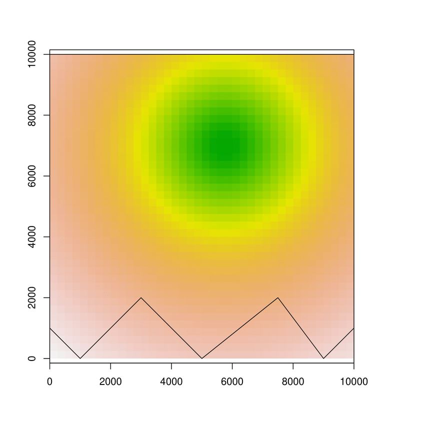
A superseding alternative is to consider the dynamical behaviour of individuals in the population
and to postulate a generic transition model across the reference grid, which together with the event
location probabilities computed above, enter into a hidden Markov model (HMM) as transition and
emission models, respectively. Upon estimation of these model parameters, we can compute the
posterior location probabilities for each device d (see figure 5). Mathematical details are provided in
the appendix.
Figure 5: Animation. Event location probabilities [left] and posterior location probabilities [right]
for a given device. True position also included.
The use of HMMs in the context of this reference grid for analysis is notably versatile and pro-
vides a generic framework to deal with multiple aspects. Firstly, at this initial stage of the project,
we have defined the HMM state just as the location in the grid, but more complex states can be
possibly defined taking into account the velocity, the transport mode, or a classification of anchor
points (home, work, second residence, etc.). Secondly, the emission model (i.e. the event location
probabilities) is built independently of the transition model, which allows MNOs to concentrate the
processing of sensitive network information (antenna localizations, network parameters, etc.) on a
this concrete production step. For the HMM, only the output of this step is needed, thus making it
possible to undisclose and protect this sensitive information. Finally, the use of probabilities allows
us to take into account the uncertainty in the estimation process from the onset. Indeed, we can
define familiar accuracy indicators for the geolocation such as bias, standard deviation, and mean
squared error as with traditional survey data (see appendix).E ND - TO - END STATISTICAL PROCESS WITH MOBILE NETWORK DATA 53
4.3 Deduplication
Since we focus on estimating population counts of individuals, not of mobile devices, we need to
detect which terminals are carried over by the same individuals. We call it device multiplicity. The
(n)
goal is to compute a device-multiplicity probability pd for each device d to be carried over by the
same individual together with a total of n devices. In our simulated scenario, for computational ease,
(1) (2) (1)
with limit the number of devices per individual to 2. Thus, we aim at computing (pd , pd = 1 − pd ),
i.e. the probability that a device d belongs to an individual with 1 or 2 devices, respectively.
The problem of device duplicity has been often recognised as an overcoverage problem. It is
usually considered after the aggregation step producing number of devices per territorial area and
time interval. Once this aggregation step has been conducted, the challenge is really serious and may
easily drive us into an identifiability problem (Lehmann and Casella, 2003) in any model estimating
the number of individuals from the number of devices. The reader may easily be convinced with
a simple example. Consider a population of N (D) = 10 devices, all corresponding to a different
individual, i.e. N = 10. Consider another population of N (D) = 10 devices, where each individual has
two devices, i.e. N = 5. There is no possible statistical model using only the variable N (D) possibly
distinguishing between these two situations. In other words, we run into an identifiability problem
unless more parameters are introduced, which will require the use of auxiliary information. In this
simple case, we may think of a statistical model based on (N (D) , Rdup ) where we have introduced
another parameter Rdup standing for the duplicity rate in the population. With these variables, the
identifiability problem ameliorates, but the model complexity increases, apart from the issue about
data availability (is Rdup really available?).
This is why we recommend to address this problem before the aggregation step. This has direct
implications for the access agreements. According to this recommendation, the number of devices
is not a target dataset in the statistical process and the device multiplicity issue must be addressed
upon individual information at the device level, thus ideally in MNOs’ premises (together with the
geolocation step).
Another important consideration arises when considering uncertainty. It is important to remind
(n)
that we target at the probability pd of each device d. This probability distribution will indeed
be another intermediate distribution in the chain (1). We need to assess the uncertainty (i.e.
probabilities) and not just to conduct a classification. The relevance of this will be evident in the
aggregation step later on.
We have proposed two alternative approaches. On the one hand, we resort to Bayesian reason-
ing to test the hypothesis that two given devices d1 and d2 belong to the same individual. Let us
denote by Hdd the hypothesis that device d uniquely corresponds to an individual, whereas Hd1 d2
stands for devices d1 and d2 , d1 belonging to the same individual. Thus, we need to compute
(1)
pd = P Hdd E, Iaux , where E = {Edt }d=1,...,D
t=0,...,T is all network event information. We propose two proce-
dures:
(1)
• Pair computation.- We compute pd = 1 − maxd 0 ,d P Hdd 0 Ed , Ed 0 , Iaux , where
SJS, VOL . 2, N O . 1 (2020), PP. 41 - 7754 D. S ALGADO ET AL .
P Ed , Ed 0 |Hdd 0 ,Iaux P (Hdd 0 |Iaux )
aux
P (Hdd 0 |Ed , Ed 0 , I ) = ,
P (Ed |Hdd , Iaux ) P (Hdd |Iaux ) + P (Ed , Ed 0 |Hdd 0 , Iaux ) P (Hdd 0 |Iaux )
(4)
with P (Hdd 0 |I), P (Hdd |Iaux ) being prior probabilities and P (Ed , Ed 0 |Hdd 0 , Iaux ), P (Ed |Hdd , Iaux )
standing for the likelihoods under each hypothesis, respectively.
• One-to-one computation.- Alternatively, posing Ωd = D
S
d 0 =1 Hdd , we compute
(1) P Ed Hdd , Iaux · P Hdd Iaux
pd = P .
P Ed Hdd , Iaux · P Hdd Iaux + d 0 ,d P Ed , Ed 0 Hdd 0 , Iaux · P Hdd 0 Iaux
(5)
T0 T1 T2 T3 T4 T5 T6
E0 E ′0 E1 E ′1 E3 E ′3 E5 E ′5 E6 E ′6
Figure 6: Extended HMM to compute P (Ed , Ed 0 |Hdd 0 , Iaux ) for a given device d (subscript not included
in the graphical model).
In both procedures the probabilities P (Ed |Hdd , Iaux ), P (Ed , Ed 0 |Hdd 0 , Iaux ) are computed with the
original HMM and the extended HMM represented in figure 6, respectively. Priors are computed
incorporating prior information e.g. from the Customer Relationship Management Database or any
other complementary information (see Salgado et al., 2020, for some details).
On the other hand, instead of focusing on the network event variables Edt , we can make use of
(c)
the random location Rdt ∈ {ri }i=1,...,NT estimated according to the posterior location probabilities
γdti . Then, we can follow the same approach as the Bayesian pair computation case (4) substituting
Edt by Rdt (see Salgado et al. (2020) for details).
In figure 7 we show the results for the Bayesian one-to-one case for our illustrative example.
The ROC curves show an excellent performance for the classification of devices according to their
duplicity with values of the area under the curve (AUC) above 0.95. Using the simulated ground
truth and a threshold of 0.50 we can also notice that very few false positive cases result (and they are
due to the short period of time under analysis: basically two individuals following nearly the same
sequence of coverage areas), whereas the number of false negative cases are a bit notable. This is due
to devices of different individuals staying under the same coverage area during the time period: they
are wrongly classified as duplicity cases of analysis. Realistic time periods of analysis will hopefully
avoid these problems.E ND - TO - END STATISTICAL PROCESS WITH MOBILE NETWORK DATA 55
RSS_uniform RSS_network SDM_uniform SDM_network case FN FP TN TP
network uniform
1.00
1
RSS
0.75
0
Sensitivity
Duplicity
0.50
RSS_uniform: 0.9888
RSS_network: 0.9873
1
0.25 SDM_uniform: 0.9609
SDM
SDM_network: 0.9603
0
0.00
1.00 0.75 0.50 0.25 0.00 0.00 0.25 0.50 0.75 1.00 0.00 0.25 0.50 0.75 1.00
Specificity Device−duplicity probability
Figure 7: [Left] ROC curve for two emission models (RSS and SDM) and two HMM priors (uniform
and network). [Right] Cases for two emission models (RSS and SDM) and two HMM priors (uniform
and network).
4.4 Statistical filtering
As of this writing, this module is the less developed since more complex and realistic displacement
patterns are needed in the simulator to study and analyse different proposals. We limit ourselves to
provide a generic view. Again, we shall be focusing on analyses upon the geolocation data, i.e. upon
the network event data and location probabilities derived thereof.
First of all, the target mobile network data is assumed to be basically some form of signalling data
so that time frequency and spatial resolution are high enough as to allow us to analyse movement
data in a meaningful way. In this sense, for example, CDR data only provides information up to a
few records per user in an arbitrary day which makes virtually impossible any rigorous data-based
reasoning in this line.
The use of HMMs implicitly incorporates a time interpolation which will be very valuable for
this statistical filtering exercise. In this way we avoid the issues arising from noncontinuous traces
approaches (see e.g. Vanhoof et al., 2018, for home location algorithms). However, a wider analysis is
needed to find the optimal time scope. In turn, the spatial resolution issue is dealt with by using the
reference grid. This releases the analyst from spatial techniques such as Voronoi tessellation, which
introduces too much noise for our purposes. Nonetheless, the uncertainty measures computed
from the underlying probabilistic approach for geolocation must be taken into account to deal with
precision issues in different regions (e.g. high-density populated vs. low-density populated).
In our view, the algorithms for statistical filtering should be mainly based on quantitative
measures of movement data. In particular, from the HMMs fitted to the data (especially the
location probabilities) we propose to derive a probability-based coarse-grained trajectory per device
which will be the basis for these algorithms. Once a trajectory is assigned to each device, different
indicators and measures of movement shall be computed upon which we shall apply algorithms
to determine important concepts such as usual environment, home/work location, second home
SJS, VOL . 2, N O . 1 (2020), PP. 41 - 7756 D. S ALGADO ET AL .
location, leisure activity times and locations, etc.
A critical issue in the development of this kind of algorithms is the validation procedure. On
the one hand, the use of the simulator, once more complex and realistic displacement patterns
have been introduced, will offer us in the future a validation against the simulated ground truth.
On the other hand, with real data two main problems need to be tackled, namely (i) the use of
pseudoanonymised real data will prevent us to link mobile device records with official registers, so
only indirect aggregated validation procedures can be envisaged, and (ii) the representativity of the
tested sample of devices (e.g. using GPS signals) to validate the algorithm for the whole population
needs to be rigorously assessed.
Thus, the starting point is the construction of a probability-based coarse-grained trajectory
for each device. In our geolocation model, the state of the HMM was defined in terms of the tile
where the device is positioned. Thus, the concept of trajectory follows immediately as the time
sequence of states, in which we shall use the coordinates of each tile to build the so-called path
{(xdt0 , ydt0 ), (xdt1 , ydt1 ), . . . , (xdtN , ydtN )}, where at each time instant ti the spatial coordinates xdti and
ydti for device d are specified. In more complex definitions of states, another procedure should lead
us to deduce the path from the adopted concept of HMM state.
Given an HMM, it is well-known that at least two different methods can be approached to build
a sequence of states, i.e. a trajectory in our case. We can compute either the most probable sequence
of states or the sequence of most probable states. In mathematical terms, the former is the sequence
∗
Tdt0 :tN
= argmaxTdt P Tdt0 :tN Edt0 :tN , (6)
0 :tN
which can be computed by means of the Viterbi algorithm (see e.g. Murphy, 2012). The second
method is indeed given by
∗
Tdt 0 :tN
= argmax γ
Tdt dt0 , argmax γ
Tdt dt1 , . . . , argmaxTdt γdtN , (7)
0 1 N
where γdtj = P Tdtj Edt0 :tN are the posterior location (state) probabilities.
We choose the maximal posterior marginal (MPM) trajectory because it is more robust and
because unimodal probabilities are expected so that differences will not be large (Murphy, 2012).
Furthermore, coherence with other process modules (e.g. duplicity) using the posterior location
probabilities is favoured in this way.
Once a path is assigned to each device we can compute different indicators as well as joint mea-
sures. Following Long and Nelson (2013) (see also multiple references therein) we distinguish the
following groups of measures:
• Time geography.- This represents a framework for investigating constraints such as maximum
travel speed on movement in both the spatial and temporal dimensions. These constraints
can be capability constraints (limiting movement possibilities because of biological/physical
abilities), coupling constraints (specific locations a device must visit thus limiting movement
possibilities), and authority constraints (specific locations a device cannot visit thus also limit-
ing movement possibilities).E ND - TO - END STATISTICAL PROCESS WITH MOBILE NETWORK DATA 57
• Path descriptors.- These represent measurements of path characteristics such as velocity, ac-
celeration, turning angles. By and large, they can be characterised based on space, time, and
space-time aspects.
• Path similarity indices.- These are routinely used to quantify the level of similarity between
two paths. Diverse options exist in the literature, some already taking into account that paths
are sequences of stays and displacements (see e.g. Long and Nelson, 2013).
• Pattern and cluster methods.- These seek to identify spatialâĂŞtemporal patterns from the
whole set of paths. These are mainly used to focus on the territory rather than on individual
patterns. They also consider diverse aspects on space, time, and space-time features.
• IndividualâĂŞgroup dynamics.- This set of measures compile methods focusing on individual
device displacement within the context of a larger group of devices (e.g. a tourist within a
larger group of tourists in the same trip).
• Spatial field methods.- These are based on the representation of paths as space or space-time
fields. Different advanced statistical methods can be applied such as kernel density estimation
or spatial statistics.
• Spatial range methods.- These are focused on measuring the area containing the device dis-
placement, such as net displacement and other distance metrics.
Diverse indicators can be defined and used within each group (see Salgado et al. (2020) for pre-
liminary examples on our simulated scenario). Further analysis is needed with realistic displacement
patterns. With a selected set of movement indicators, we shall be able to provide a computational
algorithm to substantiate the concepts of usual environment, home/work location, second home lo-
cation, etc. Notice that the definition of state for the HMM could be enhanced using these concepts,
thus incorporating more information into the geolocation estimation.
4.5 Aggregation
The next step is to aggregate the preceding information at the level of territorial units of analysis.
These territorial units usually come from an administrative division of the geographical territory,
but in general terms they will be undestood as aggregation of tiles of the reference grid. In this
sense, when deciding about the choice of grid, it is highly recommended that the territorial units
of analysis are taken into account from the onset. Obviously, the smaller the tiles, the higher the
flexibility to define different granular levels of the territorial units.
The bottom line the aggregation step is to avoid making further modelling hypothesis as much as
possible. In this line, we use probability theory to define and compute the probability distribution
for the number of individuals (not devices) detected by the network using both the posterior location
and device-duplicity probabilities.
It is important to make the following general remarks about our approach. Firstly, the
aggregation is on the number of detected individuals, not on the number of devices. This is a very
important difference with virtually any other approach found in the literature (see e.g. Deville et al.,
2014; Douglass et al., 2015). We take advantage of the preceding modules working at the device
level to study in particular the duplicity in the number of some devices per individual. This has
strong implications regarding agreements with MNOs to access and use their mobile network data
for statistical purposes. The methodology devised in the preceding section to study this duplicity
(or variants thereof) needs to be applied before any aggregation. As we can easily see, working with
the number of devices instead of the number of individuals poses severe identifiability problems
SJS, VOL . 2, N O . 1 (2020), PP. 41 - 7758 D. S ALGADO ET AL .
Regions
1
2
3
4
5
6
7
8
9
10
Figure 8: Territorial regions.
requiring more auxiliary information. Let us consider an extremely simplified illustrative example.
Let us consider population U1 of 5 individuals with 2 devices each one and population U2 of 10
individuals with 1 device each one. Suppose that in order to we make our inference statement
about the number N of individuals in the population we build a statistical model relating N and
the number of devices N (d) , that is, basically we have a probability distribution PN (N (d) ) for the
number N (d) of devices dependent on the number of individuals, from which we shall infer N . In
this situation we have PN (1) = PN (2) even when N (1) , N (2) . There is no statistical model whatsoever
capable of distinguishing between U1 and U2 (see Definition 5.2 by Lehmann and Casella, 2003, for
unidentifiable parameters in a probability distribution). To cope with the duplicity of devices using
an aggregated number of devices we would need further auxiliary information, which furthermore
must be provided at the right territorial and time scales.
Secondly, we shall use the language of probability in order to carry forward the uncertainty
already present in the preceding stages all along the end-to-end process. In another words, if the
geolocation of network events is conducted with certain degree of uncertainty (due to the nature
itself of the process) and if the duplicity of a given device (carried by an individual with another
device) is also probabilistic in nature, then a priori it is impossible to provide a certain number of
individuals2 in a given territorial unit. For this reason, we shall focus on the probability distribution
of the number of individuals detected by the network and shall avoid producing a point estimation.
Notice that having a probability distribution amounts to having all statistical information about a
random phenomenon and you can choose a point estimation (e.g. with the mean, the mode or the
median of the distribution) together with an uncertainty measure (coefficient of variation, credible
intervals, etc.).
Thirdly, the problem is essentially multivariate and we must provide information for a set of
territorial units. Thus, the probability distribution which we shall provide with our proposed
aggregation step must be a multivariate distribution. Notice that this is not equivalent to providing
a collection of marginal distributions over each territorial unit. Obviously, there will be a correlation
2 Notice that this same argument is valid for the number of devices.E ND - TO - END STATISTICAL PROCESS WITH MOBILE NETWORK DATA 59
structure, the most elementary expression of which is that individuals detected in a given territorial
unit cannot be detected in another region, so that the final distribution needs to incorporate this
restriction in its construction.
Finally, the process of construction of the final multivariate distribution for the number of
detected individuals must make as few modelling assumptions as possible, if any. In case an
assumption is made (and this should be accomplished in any use of statistical models for the
production of official statistics, in our view), it should be made as explicit as possible and openly
communicated and justified. In this line of thought, we shall strongly based the aggregation
procedure on the results of preceding modules avoiding any extra hypothesis. Basically, our starting
assumptions for the geolocation and the duplicity detection will be carried forward as far as possible
without introducing new modelling assumptions of any kind.
To implement the principles outlined above, we shall slightly change the notation used in
(1) (2)
preceding chapters. Firstly we define the vectors ei = ei and ei = 12 · ei , where ei is the canonical
unit vector in RNT (with NT the number of tiles in the reference grid). These definitions are set
up under the working assumption of individuals carrying at most 2 devices in agreement with the
deduplication step. Should we consider a more general situation, the generalization is obvious,
although more computationally demanding.
(1) (2)
Next, we define the random variable Tdt ∈ {ei , ei }i=1,...,NT with probability mass function
P (Tdt |E) given by
(1) (1)
P Tdt = ei |E1:D = γdti × pd (8a)
(2) (2)
P Tdt = ei |E1:D = γdti × pd (8b)
(i)
where pd are the device-duplicity probabilities introduced in section 4.3. Notice that this is a
categorical
or multinoulli random variable. Finally, we define the multivariate random variable
Nnet
t = N net
t1 , . . . , N net
tNT providing the number of individuals Ntinet detected by the network at each
tile i = 1, . . . , NT at time instant t:
D
X
Nnet
t = Tdt . (9)
d=1
The sum spans over the number of devices filtered as members of the target population according
to section 4.4. If we are analysing, say, domestic tourism, D will amount to the number of devices
in the network classified with a domestic tourism pattern according to the algorithms designed
and applied in the preceding module. For illustrative examples, since we have not developed the
statistical filtering module yet, we shall concentrate on present population.
The random variable Nnet t is, by construction, a Poisson multinomial random variable. The
properties and software implementation of this distribution are not trivial (see e.g. Daskalakis et al.,
2015) and we shall use Monte Carlo simulation methods by convolution to generate random variates
according to this distribution.
SJS, VOL . 2, N O . 1 (2020), PP. 41 - 7760 D. S ALGADO ET AL .
The reasoning behind this proposal can be easily explained with a simplified illustrative example.
Let us consider an extremely simple scenario with 5 devices and 5 individuals (thus, none of them
carry two devices), and 9 tiles (a 3 × 3 reference grid). Let us consider that the location probabilities
(2)
γdti = γti are the same for all devices d at each time instant and each tile. In these conditions pd = 0
for all d. Let us focus on the univariate (marginal) problem of finding the distribution of the number
of devices/individuals in a given tile i. If each device d has probability γti of detection at tile i,
then the number of devices/individuals at tile i will be given by a binomial variable Binomial(5, γti ).
If the probabilities were not equal, then the number of devices/individuals would be given by
a Poisson binomial random variable Poisson-Binomial(5; γ1ti , γ2ti , γ3ti , γ4ti , γ5ti ), which naturally
generalizes the binomial distribution. If we focus on the whole multidimensional problem, then
instead of having binomial and Poisson-binomial distributions, we must deal with multinomial and
(2)
Poisson-multinomial variables. Finally, if pd , 0 for all d, we must avoid double-counting, hence
1 (2)
the factor 2 in the definition of ei .
Notice that the only assumption made so far (apart from the trivial question of the maximum
number of 2 devices carried by an individual) is the independence for two devices to be detected at
any pair of tiles i and j. This independence assumption allows to claim that the number of detected
individuals distributes as a Poisson-multinomial variable, understood as a sum of independent
multinoulli variables with different parameters. There is no extra assumption in this derivation. The
validation of this assumption is subtle, since ultimately it will depend on the correlation between
the displacement patterns of individuals in the population. If the tile size is chosen small enough,
we claim that the assumption holds fairly well and it is not a strong condition imposed on our
derivations. On the other hand, if the tiles are too large (think of an extreme case about a reference
grid being composed of whole provinces as tiles), we should expect correlations in the detection of
individuals: those living in the same province will have full correlation and those living in different
provinces will show near null correlation. Thus, the size of the tiles imposes some limitation to the
validity of the independence assumption. Even the transport network in a territory will certainly
influence these correlations. Currently, we cannot analyse quantitatively the relationship between
the size of the tiles and the independence assumption with the network data simulator because we
need both realistic simulated individual displacement patterns and simulated correlated trajectories
(probably connected to the sharing of usual environments, home/work locations, etc.).
In figure 9 we show the high-density credible intervals with α = 0.95 for the number of
individuals Nrtnet detected by the network in each region r and each time instant t. We can compare
with true values from the simulator. Deeper and wider analyses are ongoing to assess this procedure
and its relationship with the geolocation and deduplication modules.
4.6 Inference
The last step comprises the estimation of the number of individuals Nrt in the target population
in each region r at each time instant t. Notice that we aim at estimating also those individuals not
detected by the network, namely, those subscribers of other MNOs and those not having a mobile
device. To avoid identifiability problems, we need to make use of auxiliary information. This
reg
will basically be the register-based population figures Nr and the penetration rates Prnet . Notice,
however, the different time scales of the register-based population estimates and of the network-You can also read