Towards the use of conservative thermodynamic variables in data assimilation: a case study using ground-based microwave radiometer measurements ...
←
→
Page content transcription
If your browser does not render page correctly, please read the page content below
Atmos. Meas. Tech., 15, 2021–2035, 2022
https://doi.org/10.5194/amt-15-2021-2022
© Author(s) 2022. This work is distributed under
the Creative Commons Attribution 4.0 License.

Towards the use of conservative thermodynamic variables in data
assimilation: a case study using ground-based microwave
radiometer measurements
Pascal Marquet1 , Pauline Martinet1 , Jean-François Mahfouf1 , Alina Lavinia Barbu1 , and Benjamin Ménétrier2
1 CNRM,     Université de Toulouse, Météo-France, CNRS, Toulouse, France
2 INP,   IRIT, Université de Toulouse, Toulouse, France

Correspondence: Pascal Marquet (pascal.marquet@meteo.fr, pascalmarquet@yahoo.com) and Pauline Martinet
(pauline.martinet@meteo.fr)

Received: 27 October 2021 – Discussion started: 20 November 2021
Revised: 21 January 2022 – Accepted: 28 February 2022 – Published: 5 April 2022

Abstract. This study aims at introducing two conservative          water. On the other hand, analysis increments in model space
thermodynamic variables (moist-air entropy potential tem-          (water vapour, liquid water) show significant differences be-
perature and total water content) into a one-dimensional           tween the two sets of variables.
variational data assimilation system (1D-Var) to demon-
strate their benefits for use in future operational assimilation
schemes. This system is assessed using microwave bright-           1   Introduction
ness temperatures (TBs) from a ground-based radiometer in-
stalled during the SOFOG3D field campaign, dedicated to            Numerical weather prediction (NWP) models at convective
fog forecast improvement.                                          scale need accurate initial conditions for skilful forecasts of
   An underlying objective is to ease the specification of         high impact meteorological events taking place at a small
background error covariance matrices that are highly depen-        scale such as convective storms, wind gusts or fog. Observing
dent on weather conditions when using classical variables,         systems sampling atmospheric phenomena at a small scale
making difficult the optimal retrievals of cloud and thermo-       and high temporal frequency are thus necessary for that pur-
dynamic properties during fog conditions. Background er-           pose (Gustafsson et al., 2018). Ground-based remote-sensing
ror covariance matrices for these new conservative variables       instruments (e.g. rain and cloud radars, radiometers, wind
have thus been computed by an ensemble approach based              profilers) meet such requirements and provide information
on the French convective scale model AROME, for both all-          on wind, temperature and atmospheric water (vapour and hy-
weather and fog conditions. A first result shows that the          drometeors). Moreover, data assimilation systems are evolv-
use of these matrices for the new variables reduces some           ing towards ensemble approaches where hydrometeors can
dependencies on the meteorological conditions (diurnal cy-         be initialized together with typical control variables. This
cle, presence or not of clouds) compared to typical variables      is the case for the Météo-France NWP limited area model
(temperature, specific humidity).                                  AROME (Seity et al., 2011; Brousseau et al., 2016), where,
   Then, two 1D-Var experiments (classical vs. conserva-           on top of wind (U, V ), temperature (T ) and specific humidity
tive variables) are evaluated over a full diurnal cycle char-      qv , the mass content of several hydrometeors can be initial-
acterized by a stratus-evolving radiative fog situation, using     ized (cloud liquid water ql , cloud ice water qi , rain qr , snow
hourly TB.                                                         qs and graupel qg ; Destouches et al., 2021). However, these
   Results show, as expected, that TBs analysed by the 1D-         variables are not conserved during adiabatic and reversible
Var are much closer to the observed ones than the back-            vertical motion.
ground values for both variable choices. This is especially           The accuracy of the analysed state in variational schemes
the case for channels sensitive to water vapour and liquid         highly depends on the specification of the so-called back-

Published by Copernicus Publications on behalf of the European Geosciences Union.

2022                                       P. Marquet et al.: Data assimilation using conservative thermodynamic variables

ground error covariance matrix. Background error variances          (De Angelis et al., 2016; Cimini et al., 2019) will allow for
and cross-correlations between variables are known to be            the accurate simulation of the TBs and suitable background
dependent on weather conditions (Montmerle and Berre,               error covariance matrices will be derived from an ensemble
2010; Michel et al., 2011). This is particularly the case           technique.
during fog conditions with much shorter vertical correla-              Section 2 presents the methodology (conservative vari-
tion length scales at the lowest levels and large positive          ables, 1D-Var, change of variables). Section 3 describes the
cross-correlations between temperature and specific humid-          experimental setting, the meteorological context, the obser-
ity (Ménétrier and Montmerle, 2011). In this context, Mar-          vations and the different components of the 1D-Var system.
tinet et al. (2020) have demonstrated that humidity retrievals      The results are commented in Sect. 4. Finally, conclusions
could be significantly degraded if sub-optimal background           and perspectives are given in Sect. 5.
error covariances are used during the minimization. New en-
semble approaches allow for better approximation of back-
ground error covariance matrices but rely on the capability         2     Methods
of the ensemble data assimilation (EDA) to correctly repre-
                                                                    This section presents the methodology chosen for this study.
sent model errors, which might not always be the case during
                                                                    The definition of the moist-air entropy potential temperature
fog conditions. This is why it would be of interest to exam-
                                                                    θs is introduced, as well as the formalism of the 1D-Var as-
ine, in a data assimilation context, the use of variables that
                                                                    similation system, before describing the “conservative vari-
are more suitable to times when water phase changes take
                                                                    able” conversion operator.
place.
   It is well known that most data assimilation systems             2.1    Moist-air entropy potential temperature
were based on the assumptions of homogeneity and isotropy
of background error correlations. To test these hypotheses,         The motivation for using the absolute moist-air entropy
Desroziers and Lafore (1993) and Desroziers (1997) imple-           in atmospheric science was first described by Richardson
mented a coordinate change inspired by the semi-geostrophic         (1919, 1922), and then fully formalized by Hauf and Höller
theory to test flow-dependent analyses with case studies from       (1987). The method comprises taking into account the abso-
the Front-87 field campaign (Clough and Testud, 1988),              lute value for dry air and water vapour and to define a moist-
where the local horizontal coordinates were transformed into        air entropy potential temperature variable called θs .
the semi-geostrophic space during the assimilation process.            However, the version of θs published in Hauf and Höller
Another kind of flow-dependent analyses were made by                (1987) was not really synonymous with the moist-air entropy.
Cullen (2003) and Wlasak et al. (2006), who proposed a low-         This problem has been solved with the version of Marquet
order potential vorticity (PV) inversion scheme to define a         (2011) by imposing the same link with the specific entropy
new set of control variables. Similarly, analyses on potential      of moist air (s) as in the dry-air formalism of Bauer (1908),
temperature θ were made by Shapiro and Hastings (1973)              leading to
and Benjamin et al. (1991), and more recently by Benjamin
et al. (2004) with moist virtual θv and moist equivalent θe                      θs
                                                                    s = cpd ln        + sd0 (T0 , p0 ),                       (1)
potential temperatures.                                                          T0
   The aim of the paper is to test a one-dimensional data
assimilation method that would be less sensitive to the av-         where cpd ≈ 1004.7 J K−1 kg−1 is the dry-air specific heat
erage vertical gradients of the (T , qv , ql , qi ) variables. To   at constant pressure, T0 = 273.15 K is a standard tempera-
this end, two conservative variables will be proposed, gen-         ture and sd0 (T0 , p0 ) ≈ 6775 J K−1 kg−1 is the reference dry-
eralizing previous uses of θ (as a proxy for the entropy of         air entropy at T0 and at the standard pressure p0 = 1000 hPa.
dry air) to moist-air variables suitable for data assimilation.     Because cpd , T0 and sd0 (T0 , p0 ) are constant terms, θs de-
The new conservative variables are the total water content          fined by Eq. (1) is synonymous with, and has the same phys-
qt = qv + ql + qi and the moist-air entropy potential temper-       ical properties as, the moist-air entropy s.
ature θs defined in Marquet (2011), which generalize the two           The conservative aspects of this potential temperature θs
well-known conservative variables (qt , θl ) of Betts (1973).       and its meteorological properties (in e.g. fronts, convection,
   The focus of the study will be on a fog situation from the       cyclones) have been studied in Marquet (2011), Blot (2013)
SOFOG3D field campaign using a one-dimensional varia-               and Marquet and Geleyn (2015). The links with the definition
tional data assimilation system (1D-Var) for the assimilation       of the Brunt–Väisälä frequency and the PV are described in
of observed microwave brightness temperatures (TBs) sensi-          Marquet and Geleyn (2013) and Marquet (2014), while the
tive to T , qv and ql from a ground-based radiometer. Short-        significance of the absolute entropy to describe the thermo-
range forecasts from the convective scale model AROME               dynamics of cyclones is shown in Marquet (2017) and Mar-
(Seity et al., 2011) will be used as background profiles,           quet and Dauhut (2018).
the ground-based version of the fast Radiative Transfer for            Only the first-order approximation of θs , denoted (θs )1 in
the TIROS Operational Vertical Sounder (RTTOV-gb) model             Marquet (2011), will be considered in the following, written

Atmos. Meas. Tech., 15, 2021–2035, 2022                                              https://doi.org/10.5194/amt-15-2021-2022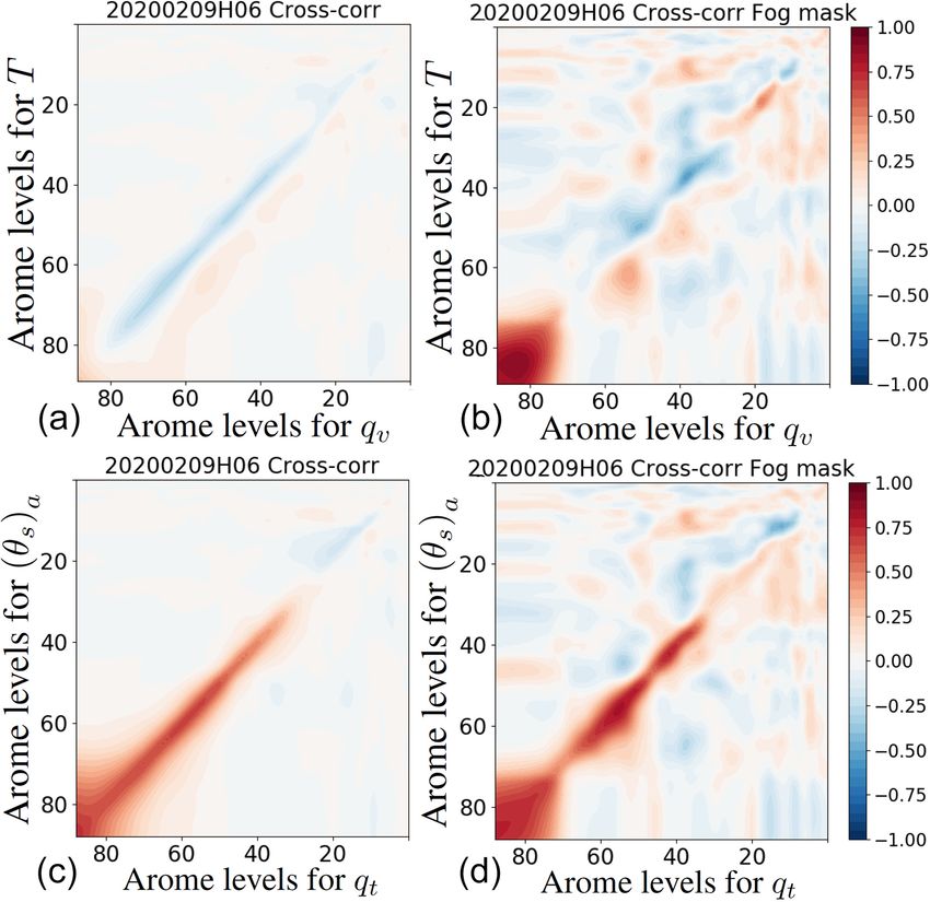
P. Marquet et al.: Data assimilation using conservative thermodynamic variables                                                   2023

as                                                                         Although it should be possible to use (θs )1 as a control
                                                                      variable for assimilation, it appeared desirable to define an
                         Lvap ql + Lsub qi
θs ≈ (θs )1 = θ exp −                      exp (3r qt ) ,        (2)    additional approximation of this variable for a more “regu-
                              cpd T                                     lar” and more “linear” formulation, insofar as tangent-linear
                                                                        and adjoint versions are needed for the 1D-Var system. Con-
where θ = T (p/p0 )κ is the dry-air potential temperature, p
                                                                        sidering the approximation exp(x) ≈ 1 + x for the two expo-
the pressure, κ ≈ 0.2857 and Lvap (T ) and Lsub (T ) the latent
                                                                        nentials in Eq. (2), neglecting the second-order terms in x 2 ,
heat of vaporization and sublimation respectively. The expla-
                                                                        also neglecting the variations of Lv (T ) with temperature and
nation for 3r follows later in the section.
                                                                        assuming a no-ice hypothesis (qi = 0), the new variable is
    The first term θ on the right-hand side of Eq. (2) leads to
                                                                        written as
a first conservation law (invariance) during adiabatic com-
pression and expansion, with joint and opposite variations
                                                                                                 Lvap (T0 ) ql

of T and p keeping θ constant. Here lies the motivation for             (θs )a = θ 1 + 3r qt −                   ,                   (3)
                                                                                                     cpd T
using θ to describe dry-air convective processes, also used                           κ
in data assimilation systems by Shapiro and Hastings (1973)                       1 p0
                                                                        (θs )a =                cpd (1 + 3r qt ) T − Lvap (T0 ) ql , (4)
and Benjamin et al. (1991).                                                      cpd p
    The first exponential on the right-hand side of Eq. (2) ex-
plains a second form of conservation law. Indeed, this expo-            where Lvap (T0 ) ≈ 2501 kJ kg−1 . This formulation corre-
nential is constant for reversible and adiabatic phase changes,         sponds to Sm /cpd , where Sm is the moist static energy de-
for which d(cpd T ) ≈ d(Lvap ql + Lsub qi ) due to the approxi-         fined in Marquet (2011, Eq. 73) and used in the European
mate conservation of the moist static energy cpd T −Lvap ql −           Centre for Medium-Range Weather Forecasts (ECMWF)
Lsub qi , and therefore has joint variations of the numerator           NWP global model by Marquet and Bechtold (2020).
and denominator and a constant fraction into the first expo-               The new potential temperature (θs )a remains close to (θs )1
nential. It should be mentioned that the product of θ by this           (not shown) and keeps almost the same three conservative
first exponential forms the Betts (1973) conservative variable          properties described for (θs )1 . This new conservative variable
θl , which is presently used together with qt to describe the           (θs )a will be used along with the total water content qt = qv +
moist-air turbulence in general circulation models (GCMs)               ql in the data assimilation experimental context described in
and NWP models.                                                         the following sections.
    While the variable θl was established with the assumption
of a constant total water content qt in Betts (1973), the second        2.2   1D-Var formalism
exponential in Eq. (2) sheds new light on a third and new
conservation law, where the entropy of moist air can remain             The general framework describing the retrieval of atmo-
constant despite changes in the total water qt . This occurs in         spheric profiles from remote-sensing instruments by statisti-
regions where water-vapour turbulence transport takes place,            cal methods can be found in Rodgers (1976). In the following
or via the evaporation process over oceans, or at the edges of          we present the main equations of the one-dimensional vari-
clouds via entrainment and detrainment processes.                       ational formalism. Additional details are given in Thépaut
    We consider here “open-system” thermodynamic pro-                   and Moll (1990), who developed the first 1D-Var inversion
cesses, for which the second exponential takes into account             applied to satellite radiances using the adjoint technique.
the impact on moist-air entropy when the changes in specific               The 1D-Var data assimilation system searches for an op-
content of water vapour are balanced, numerically, by oppo-             timal state (the analysis) as an approximate solution of the
site changes of dry air, namely with dqd = −dqt 6 = 0. In this          problem minimizing a cost function J defined by
case, as stated in Marquet (2011), the changes in moist-air
                                                                               1
entropy depend on reference values (with subscript “r”) ac-             J (x) = (x − x b )T Bx −1 (x − x b )
cording to d[qd (sd )r + qt (sv )r ], and thus with (sd )r and (sv )r          2
                                                                               1
being constant and with the relation qd = 1 − qt , leading to                 + [y − H(x)]T R−1 [y − H(x)].                         (5)
[(sv )r − (sd )r ] dqt .                                                       2
    This explains the new term 3r = [(sv )r − (sd )r ]/cpd ≈
                                                                        The symbol T represents the transpose of a matrix.
5.869 ± 0.003, which depends on the absolute reference en-
                                                                           The first (background) term measures the distance in
tropies for water vapour (sv )r ≈ 12671 J K−1 kg−1 and dry air
                                                                        model space between a control vector x (in our study, T ,
(sd )r ≈ 6777 J K−1 kg−1 . This also explains that these open-
                                                                        qv and ql profiles) and a background vector x b , weighted by
system thermodynamic effects can be taken into account to
                                                                        the inverse of the background error covariance matrix (Bx )
highlight regimes where the specific moist-air entropy (s), θs
                                                                        associated with the vector x. The second (observation) term
and (θs )1 can be constant despite changes in qt , which may
                                                                        measures the distance in the observation space between the
decrease or increase on the vertical (see Marquet, 2011, for
                                                                        value simulated from the model variables H(x) (in our study,
such examples).
                                                                        the RTTOV-gb model) and the observation vector y (in our

https://doi.org/10.5194/amt-15-2021-2022                                                  Atmos. Meas. Tech., 15, 2021–2035, 2022
2024                                       P. Marquet et al.: Data assimilation using conservative thermodynamic variables

study, a set of microwave TBs from a ground-based radiome-              Then, its gradient given by Eq. (6) becomes
ter), weighted by the inverse of the observation error covari-
                                                                                               T T −1
ance matrix (R). The solution is searched iteratively by per-       ∇z J (z) = B−1
                                                                                z (z − zb ) − L H R [y − H(L(z))],            (12)
forming several evaluations of J and its gradient:
                                                                    where LT is the adjoint of the conversion operator L.
∇x J (x) = Bx −1 (x − xb ) − HT R−1 [y − H(x)],              (6)       The second term on the right-hand side of Eqs. (11) and
where H is the Jacobian matrix of the observation opera-            (12) indicates that the conversion operator L is needed to
tor representing the sensitivity of the observation operator to     compute the TBs from the observation operator H. Indeed
changes in the control vector x (HT is also called the adjoint      RTTOV-gb requires profiles of temperature, specific humid-
of the observation operator).                                       ity and liquid water content as input quantities. This space
                                                                    change is required at each step of the minimization process.
2.3    Conversion operator                                          For the computation of the gradient of the cost function ∇z J ,
                                                                    the linearized version (adjoint) of L is also necessary. In
The 1D-Var assimilation defined previously with the vari-           practice, the operator LT provides the gradient of the TBs
ables x = (T , qv , ql ) can be modified to use the conservative    with respect to the conservative variables, knowing the gra-
variables z = ((θs )a , qt ). A conversion operator that projects   dient with respect to the classical variables.
the state vector from one space to the other can be written as
x = L(z). In the presence of liquid water ql , an adjustment
to saturation is made to separate its contribution to the total     3     Experimental set-up
water content qt from the water-vapour content qv . This is
equivalent to distinguishing the “unsaturated” case from the        The numerical experiments to be presented afterwards will
“saturated” one. Therefore, starting from initial conditions        use measurements made during the SOFOG3D field exper-
(TI , qI ) = (T , qv ) and using the conservation of (θs )a given   iment (https://www.umr-cnrm.fr/spip.php?article1086, last
by Eq. (4), we look for the variable T ∗ such that                  access: 31 March 2022; SOuth west FOGs 3D experiment
                                                                    for processes study) that took place from 1 October 2019 to
T ∗ + α qsat (T ∗ ) = TI + α qI ,                            (7)    31 March 2020 in south-western France to advance under-
                                                                    standing of small-scale processes and surface heterogeneities
where
                                                                    leading to fog formation and dissipation.
         Lvap (T0 )                                                    Many instruments were located at the Saint-Symphorien
α=                     ,                                     (8)
      cpd (1 + 3r qt )                                              super-site (Les Landes region), such as a HATPRO (Hu-
and qsat (T ∗ ) is the specific humidity at saturation.             midity and Temperature PROfiler, Rose et al., 2005), a
  For the unsaturated case (qv < qsat (T ∗ )), we obtain the        95 GHz BASTA Doppler cloud radar (Delanoë et al., 2016), a
variables (T , qv , ql ) directly from Eq. (4):                     Doppler lidar, an aerosol lidar, a surface weather station and
                                                                    a radiosonde station. One objective of this campaign was to
ql = 0,      q v = qt ,                                             test the contribution of the assimilation of such instrumenta-
                                                                    tion on the forecast of fog events by NWP models.
and
                     κ
                 p             1                                    3.1    Conditions on 9 February 2020
T = (θs )a                           .                       (9)
                 p0        1 + 3r qt
                                                                    This section presents the experimental context of 9 Febru-
  For the saturated case (qv ≥ qsat (T ∗ )), we write               ary 2020 at the Saint-Symphorien site characterized by (i) a
ql = qt − qsat (T ∗ ),                                              radiative fog event observed in the morning and (ii) the de-
                                                                    velopment of low-level clouds in the afternoon and evening.
and                                                                    Figure 1 shows a time series of cloud radar reflectivity
qv = qsat (T ∗ ).                                           (10)    profiles (W-band at 95 GHz) measured by the BASTA instru-
                                                                    ment (Delanoë et al., 2016) in the lowest hundred metres (top
   In this situation, it is necessary to implicitly calculate the   panel) between 9 February 2020 at 00:00 UTC and 10 Febru-
temperature T ∗ , given by Eq. (7). We numerically compute          ary 2020 at 00:00 UTC. The instrument reveals a thickening
an approximation of T ∗ by using Newton’s iterative algo-           of the fog between 00:00 UTC and 04:00 UTC (9 February
rithm.                                                              2020). The fog layer thickness is located between 90 and
   Taking into account this change of variables, the cost func-     250 m. After 04:00 UTC, the fog layer near the ground rises,
tion can be written as                                              lifting into a “stratus” type cloud (between 100 and 300 m).
          1                                                         After 08:00 UTC, the stratus cloud dissipates. In the bottom
J (z) = (z − zb )T B−1   z (z − zb )                                panel, BASTA observations up to 12 000 m (≈ 200 hPa) in-
          2
         1                                                          dicate low-level clouds after 14:00 UTC, generally between
      + [y − H(L(z))]T R−1 [y − H(L(z))].                    (11)   1000 m (≈ 900 hPa) and 2000 m (≈ 780 hPa), with a fairly
         2

Atmos. Meas. Tech., 15, 2021–2035, 2022                                              https://doi.org/10.5194/amt-15-2021-2022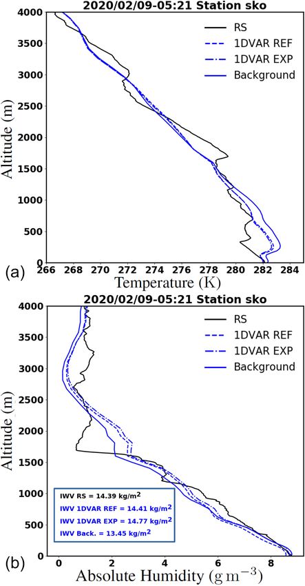
P. Marquet et al.: Data assimilation using conservative thermodynamic variables                                                   2025

Figure 1. Reflectivity profiles at 95 GHz (dBZ) measured by the BASTA cloud radar in the first 500 m (top) and up to 12 000 m altitude
(bottom), with UTC times given on the x axis, for the day of 9 February 2020 at Saint-Symphorien (Les Landes region). From http://basta.
projet.latmos.ipsl.fr/?bi=bif (last access: 31 March 2022).

good agreement with AROME short-range (1 h) forecasts                 (4), which allows the vertical gradients of θ in Fig. 2b and qv
(see Fig. 2f). Optically thin (reflectivity below 0 dBZ) high-        in Fig. 2c to often compensate each other in the formula for
altitude ice clouds are also captured by the radar.                   (θs )a . This is especially true between 980 and 750 hPa in the
   Figure 2 depicts the diurnal cycle evolution in terms of           morning between 04:00 and 10:00 UTC, and also within the
the vertical profiles of (a) absolute temperature T , (b) dry-        dry and moist boundary layers during the day.
air potential temperature θ , (c) water-vapour specific content          Note that the dissipation of the fog is associated with a ho-
qv , (d) entropy potential temperature (θs )a , (e) cloud liquid      mogenization of (θs )a in Fig. 2d from 04:00 to 05:00 UTC
water specific content ql and (f) relative humidity (RH), from        in the whole layer above, in the same way as the transition
1 h AROME forecasts (background) of 9 February 2020 at                from stratocumulus toward cumulus was associated with a
Saint-Symphorien. At this stage, it is important to note that         cancellation of the vertical gradient of (θs )1 in Fig. 6 of Mar-
the AROME model has a 90-level vertical discretization from           quet and Geleyn (2015). This phenomenon cannot be easily
the surface up to 10 hPa, with high resolution in the planetary       deduced from the separate analysis of the gradients of θ and
boundary layer (PBL) since 20 levels are below 2 km.                  qv in Fig. 2b and c. Therefore, three air mass changes can
   Figure 2e and f, for ql and RH, show two main saturated            be clearly distinguished during the day. The vertical gradi-
layers: a fog layer close to the surface between 00:00 and            ents of (θs )a are stronger during cloudy situations, first (i) at
09:00 UTC with the presence of a thin liquid cloud layer aloft        night and early morning before 04:00 UTC and just above
at 850 hPa at 00:00 UTC, and the presence of a stratocumu-            the fog, then (ii) at the end of the day above the top-cloud
lus cloud between 14:00 UTC and midnight (24:00 UTC) at               level at 800 hPa and (iii) turbulence-related phenomena in
850 hPa. During the night, the near-surface layers cool down,         between that mix the air mass and (θs )a , up to the cloudy
with a thermal inversion that sets at around 01:00 UTC and            layer tops that evolve between 950 and 800 hPa from 13:00
persists until 07:00 UTC. After the transition period between         to 17:00 UTC.
06:00 and 09:00 UTC, when the dissipation of the fog and                 The observations to be assimilated are presented in the fol-
stratus takes place, the air warms up and the PBL develops            lowing. The HATPRO MicroWave Radiometer (MWR) mea-
vertically (see the black curves plotted where vertical gradi-        sures TBs at 14 frequencies (Rose et al., 2005) between 22.24
ents of θ in Fig. 2b are large). Towards the end of the day,          and 58 GHz: 7 are located in the water-vapour absorption K-
the thickness of the PBL remains important until 24:00 UTC,           band and 7 are located in the oxygen absorption V-band (see
probably due to the presence of clouds between 800 and                the Table 1). For our study, the third channel (at 23.84 GHz)
750 hPa, which reduces the radiative cooling (see Fig. 2c and         was eliminated because of a receiver failure identified during
f for qv and RH).                                                     the campaign. In this preliminary study, we have only con-
   Figure 2d reveals weaker vertical gradients for the (θs )a         sidered the zenith observation geometry of the radiometer for
profiles, notably with contour lines often vertical and less nu-      the sake of simplicity.
merous than those of the T , θ and qv profiles in panels (a),            The H RTTOV-gb model needed to simulate the model
(b) and (c), as also shown by more extensive and more nu-             equivalent of the observations, which, together with the
merous vertical arrows in panel (d) than in panel (b). Here           choice of the control vector and the specification of the back-
we see the impact of the coefficient 3r ≈ 5.869 in Eqs. (3)–

https://doi.org/10.5194/amt-15-2021-2022                                                 Atmos. Meas. Tech., 15, 2021–2035, 2022
2026                                         P. Marquet et al.: Data assimilation using conservative thermodynamic variables

Figure 2. Vertical profiles derived from 1 h forecasts of AROME background for all hours of the day 9 February 2020 at Saint-Symphorien
(Les Landes region in France) for (a) absolute temperature T every 2 K, (b) dry-air potential temperature θ every 0.2 K, (c) water-vapour
specific content qv every 1 g kg−1 , (d) entropy potential temperature (θs )a every 0.2 K, (e) cloud liquid-water specific content ql (contoured
for 0.00001 and 0.002 g kg−1 , then every 0.1 g kg−1 above 0.1 g kg−1 ) and (f) relative humidity (RH) every 10 %. The black curves (solid
and dashed lines) represent the planetary boundary layer (PBL) heights determined from the maximum of the vertical gradients of θ. The
vertical arrows in (b) and (d) indicate areas where potential temperatures are almost homogeneous or constant along the vertical.

ground and observation error matrices, are presented in the               perimental set-up has been defined where the minimization
next section.                                                             is performed with the control vector being (T , qv , LWP). It
                                                                          will be considered as the reference, named REF. The 1D-
3.2    Components of the 1D-Var                                           Var system chosen for the present study is the one developed
                                                                          by the EUMETSAT NWP SAF (Numerical Weather Predic-
In 1D-Var systems, the integrated liquid water content, liq-              tion Satellite Application Facility), where the minimization
uid water path (LWP), can be included in the control vec-                 of the cost function is solved using an iterative procedure
tor x as initially proposed by Deblonde and English (2003)                proposed by Rodgers (1976) with a Gauss–Newton descent
and more recently used by Martinet et al. (2020). A first ex-             algorithm. During the minimization process, only the amount

Atmos. Meas. Tech., 15, 2021–2035, 2022                                                      https://doi.org/10.5194/amt-15-2021-2022
P. Marquet et al.: Data assimilation using conservative thermodynamic variables 2027
Table 1. Channel numbers, band frequencies (GHz) and observation uncertainties (K) prescribed in the observation error covariance matrix
(from Martinet et al., 2020).
Channel numbers 1 2 X 4 5 6 7
K-band frequencies (GHz) 22.24 23.04 X 25.44 26.24 27.84 31.4
K-band σo (K) 1.34 1.71 X 1.08 1.25 1.17 1.19
Channel numbers 8 9 10 11 12 13 14
V-band frequencies (GHz) 51.26 52.28 53.86 54.94 56.66 57.3 58
V-band σo (K) 3.21 3.29 1.30 0.37 0.42 0.42 0.36
of integrated liquid water is changed. In this approach, the radiometer installed at Saint-Symphorien. This section
two “moist” variables qv and LWP are considered to be in- presents and discusses three aspects of the results obtained:
dependent (no cross-covariances for background errors be- (1) the study of background error cross-correlations; (2) the
tween these variables). The second experimental framework, performance of the 1D-Var assimilation system in observa-
where the control vector is z = ((θs )a , qt ), corresponding to tion space by examining the fit of the simulated TB with re-
the conservative variables, is named EXP. The numerical as- spect to the observed ones; and (3) the performance of the
pects of the 1D-Var minimization are kept the same as in 1D-Var assimilation system in model space in terms of anal-
REF. ysis increments for temperature, specific humidity and liquid
Then, a set of reference matrices Bx (T , qv ) was estimated water content.
every hour using the EDA system of the AROME model
on 9 February 2020. These matrices were obtained by com- 4.1 Background error cross correlations
puting statistics from a set of 25 members providing 3 h
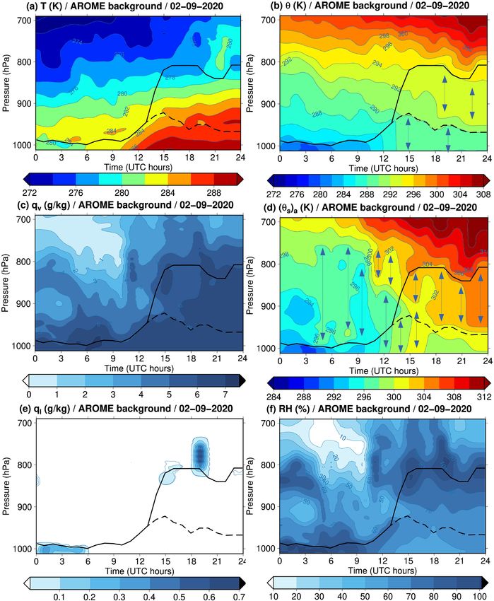
forecasts for a subset of 5000 points randomly selected in Figure 3 displays for the selected day at 06:00 UTC the cross-
the AROME domain to obtain a sufficiently large statistical correlations between T and qv (top) and between (θs )a and
sample. Then, matrices associated with fog areas, denoted qt (bottom), with (right) and without (left) a fog mask. For
Bx (T , qv )fog , were computed every hour by applying a fog the classical variables the correlations are strongly positive
mask (defined by areas where ql is above 10−6 kg kg−1 for in the saturated boundary layer with the fog mask from lev-
the three lowest model levels), in order to select only model els 75 to 90 (between 1015 and 950 hPa), while with profiles
grid points for which fog is forecast in the majority of the 25 in all-weather conditions the correlations between T and qv
AROME members. The background error covariance matri- are very weak in the lowest layers. On the other hand, the
ces Bz ((θs )a , qt ) and Bz ((θs )a , qt )fog were obtained in a sim- atmospheric layers above the fog layer exhibit negative cor-
ilar way. relations between temperature and specific humidity along
The observation errors are those proposed by Martinet the first diagonal.
et al. (2020) with values between 1 and 1.7 K for humidity When considering conservative variables, the correlations
channels (frequencies between 22 and 31 GHz), values be- along the diagonal show a consistently positive signal in the
tween 1 and 3 K for transparent channels affected by larger troposphere (below level 20 located around 280 hPa). Con-
uncertainties in the modelling of the oxygen absorption band trary to the classical variables, which are rather independent
(frequencies between 51 and 54 GHz) and values below 0.5 K in clear-sky atmospheres as previously shown by Ménétrier
for the most opaque channels (frequencies between 55 and and Montmerle (2011), the Bz matrix reflects the physical
58 GHz). link between the two new variables (shown by Eq. 4) as di-
The RTTOV model is used to calculate TBs in differ- agnosed from the AROME model. The correlations are pos-
ent frequency bands from atmospheric temperature, wa- itive with and without a fog mask. This result shows that
ter vapour and hydrometeor profiles together with surface the matrix Bz ((θs )a , qt ) is less sensitive to fog conditions
properties (provided by outputs from the AROME model). than the Bx matrix. It could therefore be possible to com-
This radiative transfer model has been adapted to simulate pute a Bz ((θs )a , qt ) matrix without any profile selection cri-
ground-based microwave radiometer observations (RTTOV- teria that would be nevertheless suitable for fog situations,
gb) by De Angelis et al. (2016). resulting in a more robust estimate. This result is key for
1D-Var retrievals which are commonly used in the commu-
nity of ground-based remote-sensing instruments to provide
4 Numerical results databases of vertical profiles for the scientific community. In
fact, the accuracy of 1D-Var retrievals is expected to be more
The 1D-Var algorithm was tested on the day of 9 Febru- robust with less flow-dependent B matrices.
ary 2020 with observations from the HATPRO microwave
https://doi.org/10.5194/amt-15-2021-2022 Atmos. Meas. Tech., 15, 2021–2035, 20222028 P. Marquet et al.: Data assimilation using conservative thermodynamic variables
Figure 3. Background error cross-correlation matrices at Figure 4. Same as Fig. 3, but at 21:00 UTC.
06:00 UTC 9 February 2020 without (a, c) and with (b, d)
a fog mask. (a, b) Between the classical variables (T , qv ).
(c, d) Between the new conservative variables ((θs )a , qt ). The axes
correspond to the levels of the AROME vertical grid (1 at the vations can reach higher values exceeding 10 K (in the after-
top and 90 for the first level above the surface). Correlations are noon) or around −5 K (in the morning).
between −1 (blue) and 1 (red) as shown in the colour bars (the In terms of residuals, as expected from 1D-Var systems,
same for the four plots). both experiments significantly reduce the deviations of the
observed TB from those calculated using the background
profiles, especially for the first eight channels sensitive to wa-
ter vapour and liquid water. We can note that the residuals are
We also note that these background error statistics are
not as reduced for channel 9 (52.28 GHz) compared to other
less dependent on the diurnal cycle and on the meteorolog-
channels. Indeed, channels 8 and 9 (51.26 and 52.28 GHz)
ical situation (e.g. in the presence of fog at 06:00 UTC and
suffer from larger calibration uncertainties (Maschwitz et al.,
low clouds at 21:00 UTC), contrary to the Bx (T , qv ) matrix,
2013) and larger forward model uncertainties dominated by
where there is a reduction in the area of positive correlation
oxygen line mixing parameters (Cimini et al., 2018) than
in the lowest layers between 06:00 and 21:00 UTC (Fig. 4).
other temperature-sensitive channels. However, by compar-
The 1D-Var results are now assessed in observation space
ing simulated TB with different absorption models (Hewi-
by examining innovations (differences between observed and
son, 2007), or through monitoring with simulated TB from
simulated TBs) from AROME background profiles and resid-
clear-sky background profiles (De Angelis et al., 2017; Mar-
uals. In the following, we have only used background error
tinet et al., 2020), larger biases are generally observed only at
covariance matrices estimated at 06:00 UTC with a fog mask,
52.28 GHz. Consequently, the higher deviations observed in
for a simplified comparison framework of the two 1D-Var
Fig. 5 for channel 9 mostly originate from larger modelling
systems.
and calibration uncertainties, which are taken into account in
the assumed instrumental errors (prescribed observation er-
4.2 1D-Var analysis fit to observations rors of about 3 K for these two channels compared to < 1 K
for other temperature-sensitive channels) and also possibly
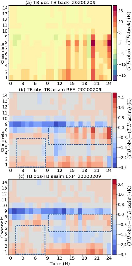
Figure 5 presents both (a) innovations and (b, c) residuals from larger instrumental biases.
obtained with the two 1D-Var systems (Fig. 5b: REF and The temperature channels used in the zenith mode are only
Fig. 5c: EXP) for the 13 channels (1, 2, 4–14) and for each slightly modified as the deviations from the background val-
hour of the day. The innovations are generally positive for ues are much smaller than for the other channels. During
water-vapour-sensitive channels during the day, and negative the second half of the day, characterized by the presence of
for temperature channels, especially in the morning. The dif- clouds around 800 hPa (see Fig. 2e and f), the residual values
ferences are mostly between −2.5 and 5 K. For channels 8, 9 are largely reduced in the frequency bands sensitive to liquid
and 10, which are sensitive to liquid water content, the inno- water for channels 6, 7 and 8, especially for EXP as shown by
Atmos. Meas. Tech., 15, 2021–2035, 2022 https://doi.org/10.5194/amt-15-2021-2022P. Marquet et al.: Data assimilation using conservative thermodynamic variables 2029
bias of 1.32 K. Both assimilation experiments reduce these
two quantities by modifying model profiles. The RMSEs
are 0.71 K for EXP and 0.72 K for REF and the biases are
−0.17 K for EXP and −0.11 K for REF. These statistics
have also been calculated by restricting the dataset to the
two dashed rectangular boxes presented in Fig. 5b and c. A
significant improvement is observed for the most sensitive
channels to liquid water in the afternoon with the RMSE de-
creasing from 4.3 K in the background to 0.57 K in REF and
0.37 K in EXP. For all computed statistics, EXP always pro-
vides the best performance in terms of RMSE. Table 2 sum-
marizes the bias and RMSE values obtained for the different
samples.
4.3 Vertical profiles of analysis increments
After examining the fit of the two experiments to the
observed TBs, we assess the corrections made in model
space. Figure 6 shows the increments of (a, b) temperature,
(c, d) specific humidity and (e, f) liquid water for the two
experiments REF (left panels) and EXP (right panels). In ad-
dition, the increments of (θs )a are shown in panels (g)–(h).
The temperature increments are mostly located in the
lower troposphere (below 650 hPa) with a dominance of neg-
ative values of small amplitude (around 0.5 K). This is con-
sistent with the negative innovations observed in the tem-
perature channels, highlighting a warm bias in the back-
ground profiles. The areas of maximum cooling take place in
cloud layers (inside the thick fog layer below 900 hPa until
09:00 UTC and around 700 hPa after 12:00 UTC). The incre-
ments are rather similar between REF and EXP, but the pos-
itive increments appear to be larger with EXP (e.g. at 08:00
and 20:00 UTC around 800 hPa).
Concerning the profiles associated with moist variables,
Figure 5. Differences in observed (channels 1, 2 and 4 to 7 located the structures show similarities between the two experiments
between 22 and 31 GHz and channels 8 to 14 located between 51 but with differences in intensity. During the night and in
and 58 GHz, HATPRO radiometer) and simulated (with RTTOV-gb) the morning, the qv increments near the surface are neg-
TBs (in Kelvin): (a) from AROME background profiles, (b) from ative. These negative increments are projected into incre-
1D-Var analyses from the REF configuration and (c) from 1D-Var ments having the same sign as T by the strong positive cross-
analyses from the EXP configuration for all hours of the day on correlations of the Bfog matrix up to 900 hPa (Fig. 3). Thus,
9 February 2020 at Saint-Symphorien (Les Landes region). The the largest negative temperature and specific humidity incre-
dashed blue boxes indicate the channels and times where EXP is ments remain confined in the lowest layers.
improved with respect to REF. Colour bars are in unit of K. Liquid water is added in both experiments between 03:00
and 07:00 UTC, close to the surface, where the Jacobians
of the most sensitive channels to ql (6 to 8) have signifi-
the comparison of the pixels in the dashed rectangular boxes cant values in the fog layer present in the background (see
in Fig. 5b and c. Residuals are also slightly reduced for EXP Fig. 2e). After 14:00 UTC, values of qv between 850 and
in the morning and during the fog and low temperature pe- 700 hPa and ql around 800 hPa are enhanced in both cases,
riod for the first five channels (1, 2, 4–6) between 02:00 and with larger increments for the REF case, in particular at
08:00 UTC. 20:00 UTC and around 24:00 UTC (midnight). Most of the
In order to quantify these results for the 9 February 2020 liquid water is created in low clouds. Additionally, incre-
dataset (all hours and all channels), the bias and root mean ments of ql above 600 hPa are larger and more extended
square error (RMSE) values are computed for the back- vertically and in time in EXP, where condensation occurs
ground and the analyses produced by REF and EXP. The over a thicker atmospheric layer between 500 and 300 hPa
innovations are characterized by a RMSE of 3.20 K and a after 12:00 UTC. In the REF experiment, the creation of liq-
https://doi.org/10.5194/amt-15-2021-2022 Atmos. Meas. Tech., 15, 2021–2035, 20222030 P. Marquet et al.: Data assimilation using conservative thermodynamic variables
Table 2. Bias/RMSE (K) of the background and analyses produced by EXP and REF against MWR TB observations. Statistics are computed
either using all data or restricted to channels 1 to 5 between 02:00 and 08:00 UTC or channels 7 to 9 between 10:00 and 24:00 UTC (these
two sub-samplings are represented by the dashed rectangular boxes in Fig. 5b and c).
Background REF EXP
All data 1.3/2.2 −0.11/0.72 −0.17/0.71
Channels 1 to 6, 02:00 to 08:00 UTC 1.5/2.2 0.11/0.3 0.08/0.3
Channels 6 to 8, 10:00 to 24:00 UTC 2.7/4.3 0.16/0.57 −0.12/0.37
uid water above 500 hPa only reaches values of 0.3 g kg−1 to the RS profile. The 1D-Var increments are thus small and
sporadically, for example at 21:00 UTC. In this experimental close between the two experiments. However, we can note
set-up, condensed water can be created or removed over the that the EXP profile is slightly moister than the REF profile
whole column by means of the supersaturation diagnosed at from the surface up to 3500 m, which leads to a somewhat
each iteration of the minimization process (since RTTOV-gb better agreement with the RS profile below 1500 m. In terms
needs (T , qv , ql ) profiles for the TB computation). This is a of integrated water vapour (IWV), a significant improvement
clear advantage of EXP over REF, which keeps the vertical of the background IWV with respect to the RS IWV is ob-
structure of the ql profile unchanged from the background. In served with the difference reduced from almost 1 kg m−2 in
REF, liquid water is only added where it already exists in the the background to less than 0.4 kg m−2 in the analyses. These
background because once the LWP variable is updated, the analyses confirm the improvement brought to the model pro-
analysed ql profile is just modified proportionally to the ratio files by both the REF and EXP analysis increments, with
between the LWP of the analysis and of the background, as some enhanced improvement for EXP.
explained in more details by Deblonde and English (2003).
The profiles of increments for (θs )a show structures sim-
ilar to the increments of qv around 800 hPa and to the in- 5 Conclusions
crements of T below, where temperature Jacobians are the
largest (see Fig. 7 in De Angelis et al., 2016). The conversion The aim of this study was to examine the value of using
of T , qv and qt changes obtained with REF into (θs )a incre- moist-air entropy potential temperature (θs )a and total water
ments (Fig. 6g) highlights the main differences between the content qt as new control variables for variational assimila-
two systems. They take place around 800 hPa with larger in- tion schemes. In fact, the use of control variables less depen-
crements produced by the new 1D-Var particularly between dent on vertical gradients of (T , qv , ql , qi ) variables should
11:00 and 14:00 UTC. ease the specification of background error covariance matri-
Some radiosoundings (RSs) have been launched during ces, which play a key role in the quality of the analysis state
the SOFOG3D IOPs. As only one RS profile was launched in operational assimilation schemes.
at 05:21 UTC in the case study presented in the article, no To that end, a 1D-Var system has been used to assimi-
statistical evaluation of the profile increments can be carried late TB observations from the ground-based HATPRO mi-
out. However, we have conducted an evaluation of the analy- crowave radiometer installed at Saint-Symphorien (Les Lan-
sis increments obtained at 05:00 and 06:00 UTC (the 1D-Var des region in south-western France) during the SOFOG3D
retrievals were performed at a 1 h temporal resolution in line measurement campaign (winter 2019–2020).
with the operational AROME assimilation cycles) around the The 1D-Var system has been adapted to consider these new
RS launch time. As the AROME temperature background quantities as control variables. Since the radiative transfer
profile extracted at 06:00 UTC was found to have a verti- model needs profiles of temperature, water vapour and cloud
cal structure closer to the RS launched at 05:21 UTC, Fig. 7 liquid water for the simulation of TB, an adjustment process
compare the AROME background profile and 1D-Var anal- has been defined to obtain these quantities from (θs )a and qt .
yses performed with the REF and EXP experiments valid at The adjoint version of this conversion has been developed for
06:00 UTC against the RS profile. an efficient estimation of the gradient of the cost function.
The temperature increments are a step in the right direction Dedicated background error covariance matrices have been
by cooling the AROME background profile in line with the estimated from the EDA system of AROME. We first demon-
observed RS profile. The two 1D-Var analyses are close to strated that the matrices for the new variables are less depen-
each other, but the EXP analysis produces a temperature pro- dent on the meteorological situation (all-weather conditions
file slightly cooler compared to the REF analysis. In terms of vs. fog conditions) and on the time of the day (stable con-
absolute humidity (ρv = pv /(Rv T ), with pv the partial pres- ditions at night vs. unstable conditions during the day) lead-
sure and Rv the gas constant for water vapour), the back- ing to potentially more robust estimates. This is an important
ground profile already exhibits a similar structure compared result as the optimal estimation of the analysis depends on
the accurate specification of the background error covariance
Atmos. Meas. Tech., 15, 2021–2035, 2022 https://doi.org/10.5194/amt-15-2021-2022P. Marquet et al.: Data assimilation using conservative thermodynamic variables 2031 Figure 6. Profiles of analysis increments resulting from two 1D-Var experiments: REF (left) and EXP (right) for (a–b) T in K, (c–d) qv in g kg−1 , (e–f) ql in g kg−1 and (g–h) (θs )a in K. Colour bars have the same units (K or g kg−1 ) as the variables. matrix, which is known to highly vary with weather condi- cloud and fog areas. We also note that atmospheric incre- tions when using classical control variables. ments are somewhat different in cloudy conditions between The new 1D-Var has produced rather similar results in the two systems. For example, in the stratocumulus layer that terms of the fit of the analysis to observed TB values formed during the afternoon, the new 1D-Var induces larger when compared to the classical one using temperature, wa- temperature increments and reduced liquid water corrections. ter vapour and LWP. Nevertheless, quantitative results reveal Moreover, its capacity to generate cloud condensates in clear- smaller biases and RMSE values with the new system in low sky regions of the background has been demonstrated. As https://doi.org/10.5194/amt-15-2021-2022 Atmos. Meas. Tech., 15, 2021–2035, 2022
2032                                        P. Marquet et al.: Data assimilation using conservative thermodynamic variables

                                                                      using the new conservative variables when additional eleva-
                                                                      tion angles are included in the observation vector. Other case
                                                                      studies from the field campaign could also be examined to
                                                                      confirm our first conclusions.
                                                                         Finally, the conversion operator could be improved by ac-
                                                                      counting not only for liquid water content ql but also for ice
                                                                      water content qi (e.g. using a temperature threshold criteria).
                                                                      Indeed, inclusion of qi in the conversion operator should lead
                                                                      to more realistic retrieved profiles of cloud condensates, and
                                                                      a 1D-Var system with only ql can create water clouds at lo-
                                                                      cations where ice clouds should be present, as done in our
                                                                      experiment around 400 hPa between 15:00 and 24:00 UTC.
                                                                      However, since the frequencies of HATPRO are not sensitive
                                                                      to ice water content, the fit of simulated TBs to observations
                                                                      could be reduced. As a consequence, the synergy with an
                                                                      instrument sensitive to ice water clouds, such as a W-band
                                                                      cloud radar, would be necessary for improved retrievals of
                                                                      both qi and ql . It is worth noting that the variable (θs )a can
                                                                      easily be generalized to the case of the ice phase and mixed
                                                                      phases by taking advantage of the general definition of θs and
                                                                      (θs )1 , where Lvap ql is simply replaced by Lvap ql + Lsub qi .

                                                                      Code and data availability. The numerical code of the RTTOV-gb
                                                                      model together with the associated resources (coefficient files) can
                                                                      be downloaded from http://cetemps.aquila.infn.it/rttovgb/rttovgb.
                                                                      html (last access: 31 March 2022, Cimini et al., 2022) and
                                                                      from https://nwp-saf.eumetsat.int/site/software/rttov-gb/ (last ac-
                                                                      cess: 31 March 2022, NWP SAF, 2022a). The 1D-Var soft-
                                                                      ware has been adapted from the NWP SAF 1D-Var provided
                                                                      at https://nwp-saf.eumetsat.int/site/software/1d-var/ (last access:
                                                                      31 March 2022, NWP SAF, 2022b), available on request to
                                                                      pauline.martinet@meteo.fr. The instrumental data are available on
                                                                      the AERIS website dedicated to the SOFOG3D field experiment:
Figure 7. Vertical profiles of absolute temperature T (a, in K) and   https://doi.org/10.25326/148 (Martinet, 2021). AROME back-
absolute humidity ρv (b, in g m−3 ) for 9 February 2020 and show-     ground data are available on request to pauline.martinet@meteo.fr.
ing the RS launched at 05:21 UTC (solid black), the AROME back-       Quicklooks from the cloud radar BASTA are available at
ground valid at 06:00 UTC (solid blue) and the 1D-Var retrievals at   https://doi.org/10.25326/155 (Delanoë, 2021). The BUMP library
06:00 UTC obtained with REF (dashed blue) and EXP (dot–dashed         used to compute background error matrices, developed in the frame-
blue). Integrated water vapour (IWV) retrievals are also compared     work of the JEDI project led by the JCSDA (Joint Center for Satel-
to the RS IWV (in the blue box in the bottom panel).                  lite Data Assimilation, Boulder, Colorado), can be downloaded at
                                                                      https://doi.org/10.5281/zenodo.6400454 (Ménétrier et al., 2022).

a preliminary validation, the retrieved profiles from the 1D-         Author contributions. PMarq supervised the work of ALB, con-
Var have been compared favourably against an independent              tributed to the implementation of the new conservative variables in
observation data set (one radiosounding launched during the           the computation of new background error covariance matrices and
SOFOG3D field campaign). The new 1D-Var leads to pro-                 participated in the scientific analysis and manuscript revision. JFM
files of temperature and absolute humidity slightly closer to         developed the conversion operator and adjoint version and partici-
observations in the PBL.                                              pated in the scientific analysis and manuscript revision. PMart su-
   The encouraging results obtained from this feasibility             pervised the modification of the 1D-Var algorithm, supported the
study need to be consolidated by complementary studies.               use of the EDA to compute the background error covariance ma-
Observed TBs at lower elevation angles should be included             trices, provided the instrumental data used in the 1D-Var and par-
                                                                      ticipated in the manuscript revision. ALB adapted the 1D-Var al-
in the 1D-Var for a better constraint on temperature profiles
                                                                      gorithm and processed all the data, prepared the figures and par-
within the atmospheric boundary layer. Indeed, larger differ-         ticipated in the manuscript revision. BM developed and adapted the
ences in the temperature increments might be obtained be-
tween the classical 1D-Var system and the 1D-Var system

Atmos. Meas. Tech., 15, 2021–2035, 2022                                                 https://doi.org/10.5194/amt-15-2021-2022
P. Marquet et al.: Data assimilation using conservative thermodynamic variables 2033
BUMP library to compute the background error covariance matrices System Using ACARS Aircraft Observations, Mon.
for the 1D-Var and participated in the manuscript revision. Weather Rev., 119, 888–906, https://doi.org/10.1175/1520-
0493(1991)1192.0.CO;2, 1991.
Benjamin, S. G., Grell, G. A., Brown, J. M., Smirnova,
Competing interests. The contact author has declared that neither T. G., and Bleck, R.: Mesoscale Weather Prediction with the
they nor their co-authors have any competing interests. RUC Hybrid Isentropic-Terrain-Following Coordinate Model,
Mon. Weather Rev., 132, 473–494, https://doi.org/10.1175/1520-
0493(2004)1322.0.CO;2, 2004.
Disclaimer. Publisher’s note: Copernicus Publications remains Betts, A. K.: Non-precipitating cumulus convection and its
neutral with regard to jurisdictional claims in published maps and parameterization, Q. J. Roy. Meteor. Soc., 99, 178–196,
institutional affiliations. https://doi.org/10.1002/qj.49709941915, 1973.
Blot, E.: Etude de l’entropie humide dans un con-
texte d’analyse et de prévision du temps, Rapport de
stage d’approfondissement EIENM3, Zenodo [report],
Acknowledgements. The authors are very grateful to the two anony-
https://doi.org/10.5281/zenodo.6396371, 2013.
mous reviewers who suggested substantial improvements to the
Brousseau, P., Seity, Y., Ricard, D., and Léger, J.: Improve-
article. The instrumental data used in this study are part of the
ment of the forecast of convective activity from the AROME-
SOFOG3D experiment. The SOFOG3D field campaign was sup-
France system, Q. J. Roy. Meteor. Soc., 142, 2231–2243,
ported by METEO-FRANCE and the French ANR through the
https://doi.org/10.1002/qj.2822, 2016.
grant AAPG 2018-CE01-0004. Data are managed by AERIS, the
Cimini, D., Rosenkranz, P. W., Tretyakov, M. Y., Koshelev, M.
French national centre for atmospheric data and services. The
A., and Romano, F.: Uncertainty of atmospheric microwave
MWR network deployment was carried out thanks to support
absorption model: impact on ground-based radiometer simula-
by IfU GmbH, the University of Cologne, the Met Office, the
tions and retrievals, Atmos. Chem. Phys., 18, 15231–15259,
Laboratoire d’Aérologie, Meteoswiss, ONERA and Radiometer
https://doi.org/10.5194/acp-18-15231-2018, 2018.
Physics GmbH. MWR data have been made available, quality con-
Cimini, D., Hocking, J., De Angelis, F., Cersosimo, A., Di Paola,
trolled and processed in the framework of CPEX-LAB (Cloud
F., Gallucci, D., Gentile, S., Geraldi, E., Larosa, S., Nilo, S.,
and Precipitation Exploration LABoratory, http://www.cpex-lab.de,
Romano, F., Ricciardelli, E., Ripepi, E., Viggiano, M., Luini,
last access: 31 March 2022), a competence centre within the
L., Riva, C., Marzano, F. S., Martinet, P., Song, Y. Y., Ahn, M.
Geoverbund ABC/J with the acting support of Ulrich Löhnert,
H., and Rosenkranz, P. W.: RTTOV-gb v1.0 – updates on sen-
Rainer Haseneder-Lind and Arthur Kremer from the University of
sors, absorption models, uncertainty, and availability, Geosci.
Cologne. This collaboration is driven by the European COST ac-
Model Dev., 12, 1833–1845, https://doi.org/10.5194/gmd-12-
tions ES1303 TOPROF and CA18235 PROBE. Julien Delanoë and
1833-2019, 2019.
Susana Jorquera are thanked for providing the cloud radar quick-
Cimini, D., Hocking, J., De Angelis, F., Cersosimo, A., Di Paola,
looks used in this study for better understanding the meteorological
F., Gallucci, D., Gentile, S., Geraldi, E., Larosa, S., Nilo,
situation. Thibaut Montmerle and Yann Michel are thanked for their
S., Romano, F., Ricciardelli, E., Ripepi, E., Viggiano, M.,
support on the use of the AROME EDA to compute background er-
Luini, L., Riva, C., Marzano, F. S., Martinet, P., Song, Y. Y.,
ror covariance matrices. The work of Benjamin Ménétrier is funded
Ahn, M. H., and Rosenkranz, P. W.: RTTOV-gb, CETEMPS
by the JCSDA (Joint Center for Satellite Data Assimilation, Boul-
[code], http://cetemps.aquila.infn.it/rttovgb/rttovgb.html, last ac-
der, Colorado) UCAR SUBAWD2285.
cess: 31 March 2022.
Clough, S. A. and Testud, J.: The Fronts-87 experiment and
mesoscale frontal dynamics project, WMO Bulletin, 37, 276–
Financial support. This research has been supported by the Agence 281, 1988.
Nationale de la Recherche (grant no. AAPG 2018-CE01-0004), the Cullen, M. J. P.: Four-dimensional variational data assimilation:
European COST actions (ES1303 TOPROF and CA18235 PROBE) A new formulation of the background-error covariance matrix
and JCSDA UCAR (SUBAWD2285). based on a potential-vorticity representation, Q. J. Roy. Meteor.
Soc., 129, 2777–2796, https://doi.org/10.1256/qj.02.10, 2003.
De Angelis, F., Cimini, D., Hocking, J., Martinet, P., and Kneifel,
Review statement. This paper was edited by Maximilian Maahn S.: RTTOV-gb – adapting the fast radiative transfer model
and reviewed by two anonymous referees. RTTOV for the assimilation of ground-based microwave ra-
diometer observations, Geosci. Model Dev., 9, 2721–2739,
https://doi.org/10.5194/gmd-9-2721-2016, 2016.
De Angelis, F., Cimini, D., Löhnert, U., Caumont, O., Haefele, A.,
References Pospichal, B., Martinet, P., Navas-Guzmán, F., Klein-Baltink, H.,
Dupont, J.-C., and Hocking, J.: Long-term observations minus
Bauer, L. A.: The relation between “potential tem- background monitoring of ground-based brightness temperatures
perature” and “entropy”, Phys. Rev., 26, 177–183, from a microwave radiometer network, Atmos. Meas. Tech., 10,
https://doi.org/10.1103/PhysRevSeriesI.26.177, 1908. 3947–3961, https://doi.org/10.5194/amt-10-3947-2017, 2017.
Benjamin, S. G., Brewster, K. A., Brümmer, R., Jew- Deblonde, G. and English, S.: One-Dimensional Variational Re-
ett, B. F., Schlatter, T. W., Smith, T. L., and Stamus, trievals from SSMIS-Simulated Observations, J. Appl. Me-
P. A.: An Isentropic Three-Hourly Data Assimilation
https://doi.org/10.5194/amt-15-2021-2022 Atmos. Meas. Tech., 15, 2021–2035, 2022You can also read