Using multidimensional speckle dynamics for high-speed, large-scale, parallel photonic computing
←
→
Page content transcription
If your browser does not render page correctly, please read the page content below
Using multidimensional speckle dynamics for high-speed,
                                                             large-scale, parallel photonic computing
                                                                       Satoshi Sunada1,2 , Kazutaka Kanno3 , and Atsushi Uchida3
                                                           1 Faculty  of Mechanical Engineering, Institute of Science and Engineering, Kanazawa University
                                                                                  Kakuma-machi Kanazawa, Ishikawa 920-1192, Japan
                                                     2 Japan Science and Technology Agency (JST), PRESTO, 4-1-8 Honcho, Kawaguchi, Saitama 332-0012, Japan
                                                                        3 Department of Information and Computer Sciences, Saitama University,

                                                                          255 Shimo-Okubo, Sakura-ku, Saitama City, Saitama, 338-8570, Japan.

                                                          The recent rapid increase in demand for data processing has resulted in the need for novel machine
                                                      learning concepts and hardware. Physical reservoir computing and an extreme learning machine are
                                                      novel computing paradigms based on physical systems themselves, where the high dimensionality and
arXiv:2104.00311v1 [physics.optics] 1 Apr 2021

                                                      nonlinearity play a crucial role in the information processing. Herein, we propose the use of multidi-
                                                      mensional speckle dynamics in multimode fibers for information processing, where input information
                                                      is mapped into the space, frequency, and time domains by an optical phase modulation technique.
                                                      The speckle-based mapping of the input information is high-dimensional and nonlinear and can be
                                                      realized at the speed of light; thus, nonlinear time-dependent information processing can successfully
                                                      be achieved at fast rates when applying a reservoir-computing-like-approach. As a proof-of-concept,
                                                      we experimentally demonstrate chaotic time-series prediction at input rates of 12.5 Gigasamples per
                                                      second. Moreover, we show that owing to the passivity of multimode fibers, multiple tasks can be si-
                                                      multaneously processed within a single system, i.e., multitasking. These results offer a novel approach
                                                      toward realizing parallel, high-speed, and large-scale photonic computing.

                                                 1    Introduction
                                                 Reservoir computing (RC) [1, 2, 3] and an extreme learning machine (ELM) [4] are novel neuro-inspired
                                                 computing methods that use high-dimensional and nonlinear systems, e.g., neural networks, to process
                                                 input information. Unlike a conventional neural network, internal networks are fixed, and only the
                                                 readout weights are trained, which greatly simplifies the training method and enables easy hardware
                                                 implementation. To date, a variety of physical implementations of RC and ELM, including optoelectronic
                                                 and photonic systems [5], memristors [6], spin waves [7], and soft-robots [8], have been proposed, and
                                                 have demonstrated a performance comparable with that of digital computing based on other algorithms
                                                 in a series of benchmark tasks, including time-series prediction, wireless channel equalization, and image
                                                 and phoneme recognition [9].
                                                     Photonics-based RC is of particular interest. The use of photonic systems for RC implementation is
                                                 expected to accelerate recurrent neural network processing with low energy costs [10, 11]. Most photonic
                                                 RC systems are based on delayed feedback structures, which can be simply realized using a nonlinear
                                                 device with a time-delayed feedback loop [12, 13, 14, 15, 16, 17, 18]. Based on a time-multiplexing
                                                 technique [19, 20], the sampled signals of the nonlinear device are used as virtual neurons (network
                                                 nodes) for information processing. With this approach, most complex tasks can be solved with few
                                                 errors; however, these systems suffer from an inherent trade-off between the number of neurons and the
                                                 required processing time.
                                                     Meanwhile, significant progress has been made with various multiplexing approaches that utilize
                                                 other degrees of freedom of light, i.e., space and wavelength, to overcome the above trade-off [21, 22,
                                                 23, 24, 25, 26, 27]. Most multiplexing techniques are based on optical data transportation techniques
                                                 used for optical fiber communication and have the potential to realize high-speed parallel operation.
                                                 Spatial multiplexing schemes, based on optical node arrays, have been used for RC in silicon photonic
                                                 chips and have demonstrated high-speed processing of the bit header recognition at up to 12.5 Gbit/s
                                                 [21]. To generate a larger number of spatial nodes (i.e., a larger network scale), the use of speckles
                                                 generated from light scattering [24] and multimode waveguides [25], and diffractively coupled systems
                                                 [26], have been proposed, demonstrating good performance even for complex tasks, such as chaotic time-
                                                 series prediction. As other approaches, frequency multiplexing schemes have also been proposed, where
                                                 the amplitude and phase of the frequency sidebands of a laser in a fiber loop are used as reservoir
                                                 nodes, demonstrating nonlinear channel equalization and speech recognition [27]. These approaches are
                                                 promising; however, there are certain limitations. For example, the constructions of the abovementioned
                                                 spatial multiplexing networks essentially involve a direct trade-off between parallelism and footprint. In
                                                 frequency multiplexing, the number of nodes may be practically limited by the amplitudes or bandwidth
                                                 of the electronic modulators.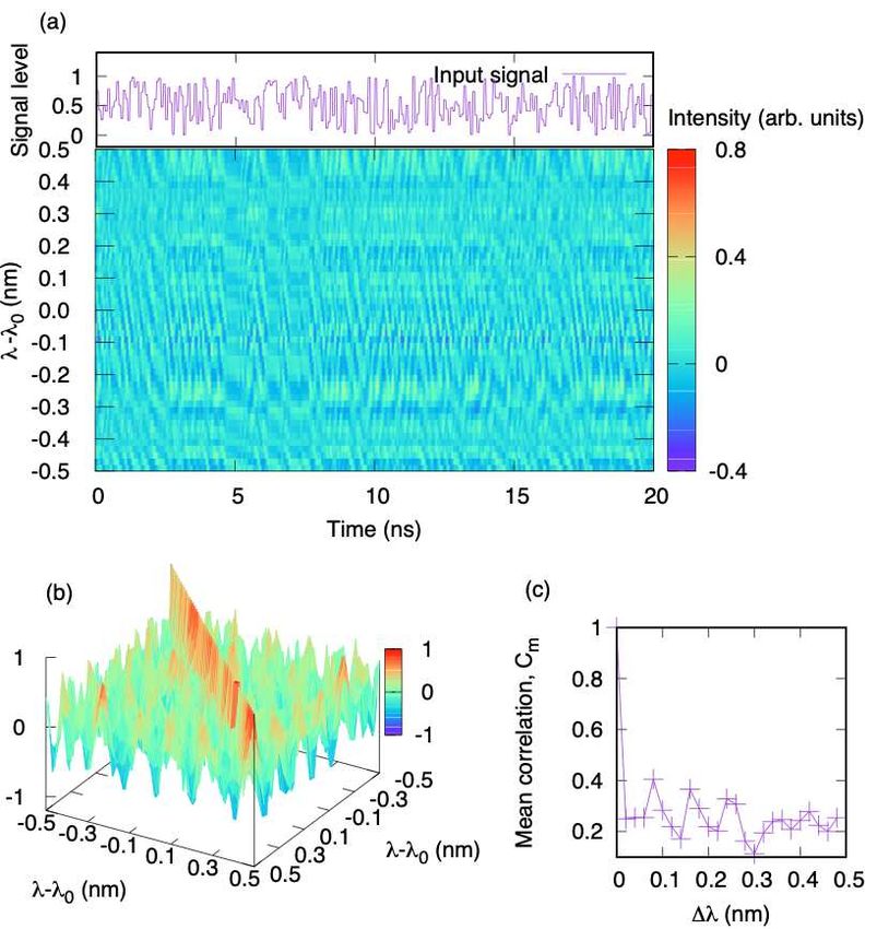
Herein, we propose a new approach to photonic parallel information processing based on high-
dimensional speckle dynamics generated from multimode fibers. This approach easily enables the com-
bined use of space, wavelength, and time multiplexing to achieve high-speed, large-scale, and parallel
processing. In the proposed system, high nonlinearity required to process nonlinear tasks can be intro-
duced using fast optical phase modulation over a few Gigasamples/s (GS/s). The origin of the nonlinearity
is the nonlinear optical mapping from phase-encoded input information into speckle patterns. This differs
from other types of photonic RC using multimode fiber speckles [25], where nonlinearity is electronically
introduced. As a proof-of-concept demonstration for high-speed parallel processing, we experimentally
show that a chaotic time-series prediction can be performed at 12.5 GS/s. Moreover, the proposed ap-
proach enables a multitasking operation, i.e., simultaneous processing of a number of independent tasks
with a single photonic processing unit, using both the space- and wavelength multiplexing techniques
together. As a primitive demonstration, we also show the simultaneous processing of two independent
tasks with respect to nonlinear channel equalization.

2     Speckle dynamics in multimode fibers
2.1    Multimode fiber speckles
Multimode fibers support hundreds of guided modes with different phase velocities. For monochromatic
input light, a complex speckle pattern is generated in the intensity distribution at the end of the multimode
fiber as a result of the interference of guided modes with different phase velocities [28, 29]. A remarkable
feature of a speckle pattern is its dependence on the wavelength of the input light. The longer the fiber
length is, the more sensitive it becomes [29, 30]. This suggests that when the wavelength (frequency) of the
input light is modulated, the speckle pattern dynamically varies over time. In other words, information
encoded by the wavelength modulation of the input light can be mapped as dynamically varying speckle
patterns. See the Appendix for the theoretical model.

2.2    Experimental setup
Figure 1(a) shows the experimental setup used to generate and measure the modulation-induced speckle
dynamics in a multimode fiber. We used a commercially available step-index multimode fiber with a
core diameter of 50 µm, numerical aperture (NA) of 0.22, and length of 10 m. The multimode fiber
supports approximately 250 guided modes at an input wavelength of λ0 = 1550 nm. The multimode fiber
was covered with an insulator to reduce the effects of thermal fluctuation and mechanical vibration. A
narrow-linewidth tunable laser (Alnair Labs, TLG-200, 100 kHz linewidth, 10 mW) was used as a light
source. The laser light was phase-modulated using a phase modulator (EO Space, AX-0MSS-20-LV, 16
GHz bandwidth) to encode an input signal, which was generated by an arbitrary waveform generator
(Tektronix, AWG70002A, 25 GS/s), as an instantaneous frequency. The maximum phase modulation
was approximately 0.9π. The modulated light was sent through a polarization-maintaining single-mode
fiber to the multimode fiber. We used a lensed fiber (spot size of ∼ 2 µm with a working distance
of ∼ 10 µm) as a probe to measure the time-variation of the output near the focal position at the
end of the multimode fiber, and the output was sent to a photodetector (New Port, 1554-B, 12 GHz
bandwidth) through an optical fiber amplifier (FiberLabs, AMP-FL80133-CB) and measured using a
digital oscilloscope (Tektronix, DPO71604B, 50 GS/s, 16 GHz bandwidth).
    To obtain the time-variation of the speckle pattern, the measurement position was repeatedly changed
by changing the position of the lensed fiber in parallel with the cross-section of the fiber end [Fig. 1(b)]
with a micro-positioning stage, whereas the input light was repeatedly modulated using the same signal.
The origins of the time variation of the output signals at each measurement position were matched by
adjusting each trigger signal to reconstruct the intensity patterns at each time. This method is effective
because a multimode fiber is passive with respect to the input, and the output demonstrates consistency
for the same inputs [31].

2.3    Speckle dynamics
Figure 2(a) shows an instance of the time variation of the intensity pattern measured by the above
method, where the phase of the input light was modulated at 12.5 GS/s with a pseudorandom sequence
and each intensity signal was measured along the x−axis shown in Fig. 1(b). The intensity pattern varies
in a nonlinear manner, according to the input signal. The nonlinearity originates from the relationship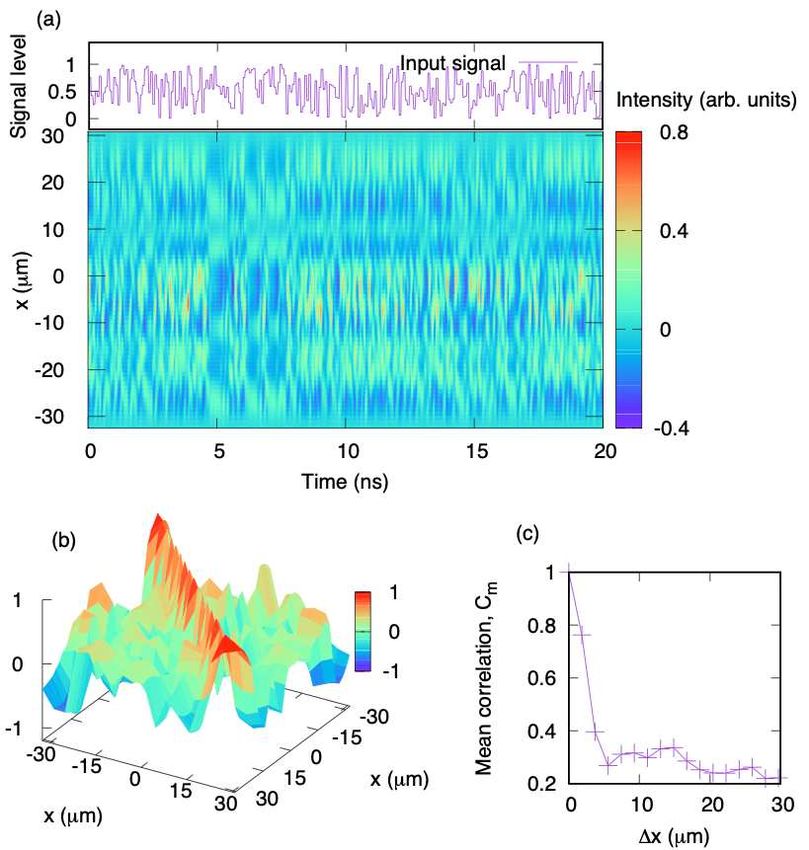
Figure 1: (a) Experimental setup for generating speckle dynamics using a multimode fiber. ISO, optical
isolator; Amp, electric amplifier; AWG, arbitrary waveform generator; PM, phase modulator; MMF,
multimode fiber; OA, optical amplifier; PD, photodetector; OSC, digital oscilloscope. A porlarization-
maintaining single-mode fiber was coupled to the MMF through a standard FC/APC mating sleeve. The
fiber probe (lensed fiber) was adjusted to measure the speckle at the end of the multimode fiber using
a five-axis positioning stage. (b) Schematic of the cross-section at the end of the multimode fiber. The
origin of the xy−axis was set as the center of the core layer.

between the input signal and output intensity signal, i.e., the input signal is encoded with the phase
modulation, whereas the output is obtained as an intensity signal (see the Appendix). Considering that
the computational capacity of the system depends on the number of linearly independent signals measured
in the system [32], we measured the correlation between two signals measured at different positions, i.e.,

                                           h[φλ0 (x, t) − φ̄λx0 ][φλ0 (x′ , t) − φ̄λx′0 ]iT
                             C(x, x′ ) =                                                    ,           (1)
                                                              σx σx′

where φλ0 (x, t) represents the intensity measured at position x at time t for input wavelength λ0 . Here,
              RT
hf iT = 1/T 0 f dt denotes the mean of f over measurement time T . In addition, φ̄λx0 and σx are
the mean and standard deviation of φλ0 (x, t), respectively. The correlation C(x, x′ ) decays for large
∆x =R |x′ − x|, as shown in Fig. 2(b). To clarify this, we calculated the mean correlation value Cm (∆x) =
1/D |C(x, x + ∆x)|dx and plot Cm (∆x) in Fig. 2(c). Here, Cm (∆x) sufficiently decays when ∆x > 4
µm for the multimode fiber used in our experiment. We use the output signals sampled at the interval
∆x ≈ 4 µm for information processing, as discussed in Sec. 3.1.

2.4    Frequency dependence
The speckle dynamics depends on the wavelength (frequency) of the input light, and a variety of dynamics
can be generated with different wavelengths in parallel. To confirm this, we varied the wavelength λ of
the input light around λ0 = 1550 nm and measured the intensity variation from the multimode fiber. In
the results shown in Fig. 3(a), the input light is phase-modulated with the same pseudorandom sequence
at 12.5 GS/s. As can be seen in the figure, various time variations are obtained, depending on the input
wavelength λ. We also measured the correlation,
                                                             ′                 ′
                                     h φλ (x0 , t) − hφλx0 i [φλ (x0 , t) − hφλx0 i]iT

                                 ′
                          C(λ, λ ) =                                                   ,                (2)
                                                           σλ σλ′

where φλ (x0 , t) represents the intensity measured at x = xR0 and y ≈ 0 for input wavelength λ [Fig. 3(b)].
Figure 3(c) shows the mean correlation Cm (∆λ) = 1/Dλ |C(λ, λ + ∆λ)|dλ. Here, Cm (∆λ) sufficiently
decays when ∆λ > 0.02 nm for the multimode fiber. ∆λ of 0.02 nm corresponds to lower bounds for the
parallel generation of different speckles and modulation bandwidth for information encoding with input
lights of different wavelengths. The correlation Cm (∆λ) can more rapidly decay with an increase in the
length of the multimode fiber [30], and a variety of dynamics that are more sensitive to the wavelength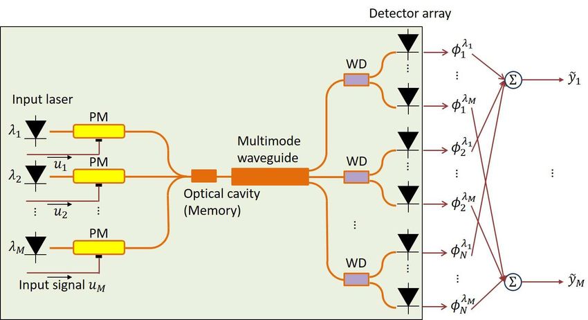
Figure 2: (a) Input signal u (upper panel) and output intensity signals φλ0 (x, t) (bottom panel) measured
at the end of the multimode fiber by scanning using a lensed fiber probe along the x−axis shown in Fig.
1(b) (see Visualization 1). The input rate 1/τ was set to 12.5 GS/s. The input signal u is displayed
as a function of time t = nτ , and the origin of time (t = 0) is adjusted to that for the output signals
for display purposes. (b) Correlation map C(x, x′ ) between the output signals φλ0 (x, t) and φλ0 (x′ , t),
which were measured at fiber positions x and x′ , respectively. (c) Mean correlation Cm as a function of
∆x = |x − x′ |. The correlation sufficiently decays when ∆x > 4 µm.
can be obtained. This result suggests that with multiple light sources of different wavelengths, the input
information can be encoded even within the wavelength domain with a multiplexing technique, and
parallel information processing is enabled, as demonstrated in Sec. 4.

Figure 3: (a) Time series of input signal u (upper panel) and output intensity signals φλ (x0 , t) (bottom
panel) measured at the fixed position x0 by changing the wavelength λ of the light source. In (a), the
input signal u is displayed as a function of time t = nτ , and the origin of time (t = 0) is adjusted
                                                                                     ′
to that for the output signals for display purposes. (b) Correlation map C(λ, λ ) between the output
                          ′                                                              ′
signals φλ (x0 , t) and φλ (x0 , t). (c) Mean correlation Cm as a function of ∆λ = |λ − λ |. The correlation
sufficiently decays when ∆λ > 0.02 nm.

3     Information processing based on speckle dynamics
3.1    Method
As demonstrated in the previous section, the use of a multimode fiber enables high-dimensional and
nonlinear mapping of the input information in the speckle patterns. We use the mapping properties
based on multimode fibers to process time-dependent input information in the following ways: The input
light is phase-modulated with a signal, u(n) (n ∈ {1, 2, · · · }), where u(n) holds for the time interval τ . The
output intensity signals, φλi 0 (t) = |E(r i , t)|2 , from the multimode fiber are measured at r i = (xi , yi ) with
steps ∆x = ∆y ≈ 4 µm in the xy-plane [Fig.1(b)] at the sampling time t = nτ , where i ∈ {1, 2, · · · , N }
is the index of the measurement position. The readout is given by the following:
                                                       N
                                                       X
                                             ŷ(n) =         wi φλi 0 (nτ ),                                    (3)
                                                       i=1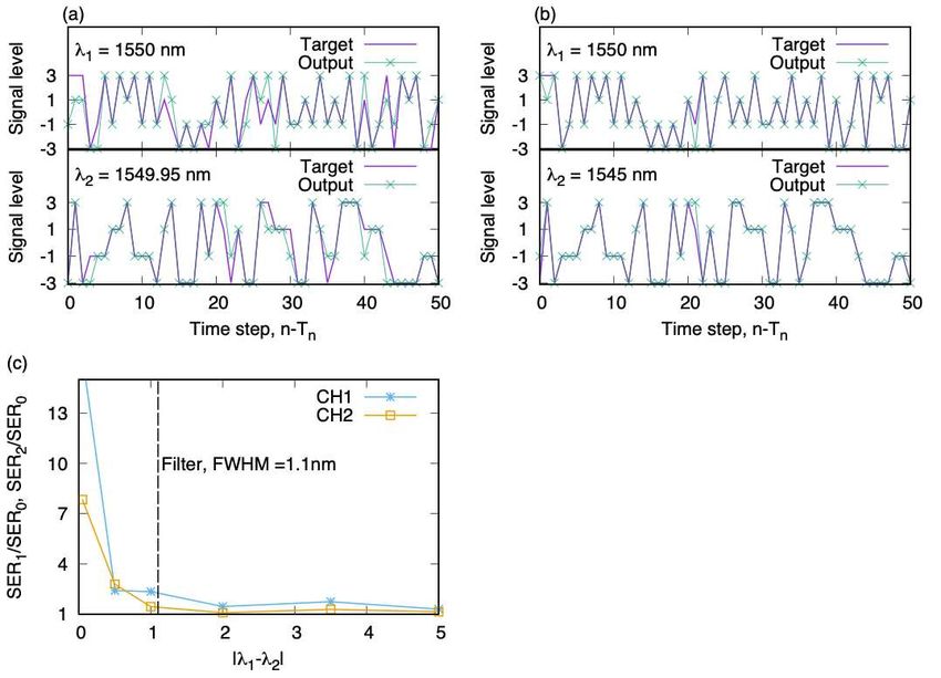
where wi is a readout weight. The goal of the processing is to approximate a functional relationship
between the input signal u(n) and target y(n) using ŷ(n). To this end, a finite set of training data
{u(n), y(n)}Tn=0
n
is utilized to calculate the optimal readout weights. This is performed through a simple
PTn 2
PN 2
ridge regression to minimize the error, n |y(n) − ŷ(n)| + λ i wi , where λ is the regularization
parameter to avoid an ill-conditioned problem [12].
3.2 Chaotic time-series prediction
As a demonstration of a computation application using speckle dynamics, we conducted the Santa Fe
time-series prediction task [33], which is a one-step ahead prediction task of chaotic data generated from a
far-infrared laser [see Fig. 4(a)]. In this task, the input signal u(n) corresponds to the n-th sampling point
of the chaotic waveform, and y(n) is set as the n+ 1-th sampling point, u(n+ 1). The prediction error was
evaluated using the normalized mean square error (NMSE), which is given by 1/Tn Tn=1 |y(n)−ŷ(n)|2 /σy2 ,
P n
2
where σy is the variance of the target signal y(n). We used Tn = 3000 steps for training and 1000 steps
for testing.
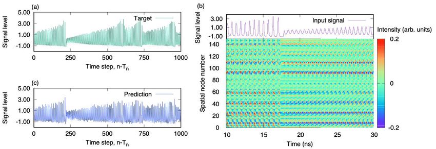
Figures 4(b) and 4(c) show the results of the measured intensity signals φλi 0 (t) and readout ŷ(n) for
an input rate of 1/τ = 12.5 GS/s of the signal u(n), respectively. According to Eq. (3), the readout ŷ(n)
was calculated with N = 150 intensity signals, which were measured at 60×60 µm2 near the fiber end.
The NMSE of the prediction was approximately 0.09, which is comparable with the NMSEs obtained for
the other photonic systems. (As an example, NMSEs of 0.106 and 0.109 have been reported for N = 388
and 124 in [13] and [16], respectively.) Unlike in other photonic information processing systems using
laser devices [13, 16], active devices are not involved in the processing in the proposed system; thus, the
response time is not limited. We expect that faster speckle dynamics and then faster processing can be
realized by increasing the input rate 1/τ .
Figure 4: (a) Target signal y(n) in the Santa Fe time-series prediction task. (b) Input signal u as a
function of time t = (n − Tn)τ (upper panel), where Tn = 3000 and τ = 0.08 ns (input rate of 1/τ = 12.5
GS/s). The lower panel shows the measured intensity signals, [φλ1 0 (t), φλ2 0 (t), · · · , φλN0 (t)], responding to
the input light with wavelength λ0 = 1550 nm, which is phase-modulated by the input signal u (see
Visualization 2). These signals are used as nodes to obtain the readout ŷ [see Eq. (3)]. (c) The readout
ŷ(n) obtained using the measured signals, [φλ1 0 (t), φλ2 0 (t), · · · , φλN0 (t)].
3.3 Using wavelength- and time-multiplexing techniques
The number of nodes N required to construct a readout ŷ [Eq. (3)] is limited by the physical dimensions of
the multimode fiber. However, as shown in Fig. 3(a), the signals generated for different input wavelengths
are expected to be used as additional nodes in the proposed system, enabling processing on a larger-scale
network. In addition, although the present experimental system does not have any memory effect, which
is crucial for time-dependent signal processing, the memory effect can be introduced by adding an optical
cavity in the system [22] or using the past information as a node in the time domain with a time-
multiplexing method [19]. In this study, we simply use the latter method, i.e, the time-multiplexing
method, and explore the availability of additional nodes in the time and wavelength domains to discuss
the potential improvement of the computational performance. We here consider the following three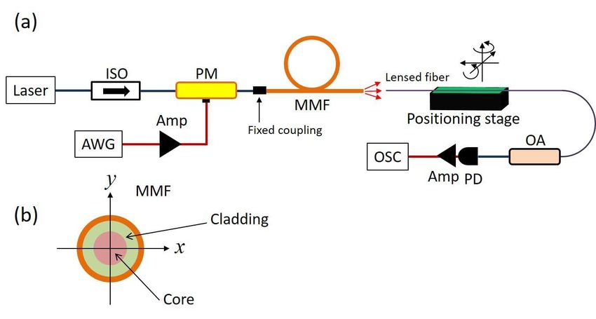
readouts:
K X
X N
ŷ1 (n) = wi,k φλi 0 [(n − k)τ ], (4)
k=0 i=1
M
K X
λ
X
ŷ2 (n) = wj,k φ0 j [(n − k)τ ], (5)
k=0 j=1
K N M
λ
X X X
ŷ3 (n) = wi,k φλi 0 [(n − k)τ ] + wj,k φ0 j [(n − k)τ ] , (6)
k=0 i=1 j=1
where the output intensity φλi 0 [(n − k)τ ] is sampled at a measurement position labeled by i for the fixed
λ
input wavelength λ0 at time t = (n − k)τ . Here, φ0 j (t) is the output intensity measured at i = 0 for
input wavelength λj (j ∈ {1, 2, · · · M }) at time t. In addition, ŷ1 (n), ŷ2 (n), and ŷ3 (n) are the readouts in
the space, wavelength, and mixed (space/wavelength) domains, respectively, and K denotes the number
of past output signals used for calculating the readouts. The readout weights wi,k and wj,k were trained
for the Santa Fe time-series prediction task.
Figure 5 shows the result of the prediction task, which was obtained by the trained readouts ŷl (n) (l ∈
{1, 2, 3}), where λ0 = 1550 nm and λj = 1549.5 + 0.02j nm. For comparison, the total number of nodes,
N + M , is fixed at 50 for all cases. As K increases, the NMSEs decrease and the prediction performance
improves. The readout ŷ1 (n) shows the best NMSE of 0.06 for K = 7, which is better than that of
other photonic RC [13, 16]. The readouts ŷ2 (n) and ŷ3 (n) exhibit a relatively improved performance,
and the best NMSE was 0.052. This improvement may be attributed to the linear independence among
λ
the signals φ0 j in the wavelength domain [Fig. 3(a)]. These results suggest that the simultaneous use of
the nodes in the space, wavelength, and time domains is effective for processing time-dependent signals.
Figure 5: Prediction errors (NMSEs) as a function of K for three readouts, ŷ1 (n), ŷ2 (n), and ŷ3 (n), which
are plotted using open circles, open squares, and crosses, respectively. The numbers of nodes used for
readouts 1, 2, and 3 are N = 50, M = 50, and N = M = 25, respectively.
4 Multitasking
Finally, we discuss the simultaneous use of the above space and wavelength multiplexing techniques,
which also allows a multitasking operation, i.e., parallel processing of numerous independent tasks, with
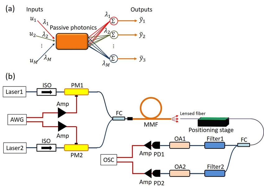
a single photonic component, that is, a multimode fiber [Fig. 6(a)]. This is enabled by the encoding of
different input information at different wavelengths because there are no nonlinear interactions between
the lights with different wavelengths. Figure 6(b) shows the experimental setup for the multitasking
operation. We used two light sources (wavelength-tunable lasers), the wavelengths of which are λ1 and
λ2 , respectively. The respective lights were then independently phase-modulated with different input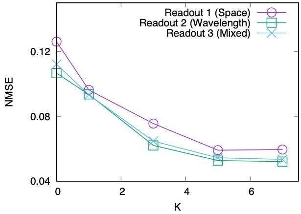
signals, u1 and u2 , and injected into a multimode fiber. The output light of λ1(2) from the multimode
fiber was detected by PD1(2) after passing through a tunable optical filter (Filter 1(2)) with a bandwidth
(full width at half maximum) of ∆ ≈ 1.1 nm, the center transmission wavelength of which was tuned at
λ1(2) and used as the spatial nodes for calculating the readouts.

Figure 6: (a) Schematic of multitasking based on passive photonics. Each input signal uj (j ∈
{1, 2, · · · , M }) is encoded as optical signals with wavelength λj and is independently processed in a
single photonic component (multimode fiber) to obtain the readout ỹi . (b) Experimental setup used for
multitasking operation based on a multimode fiber. Two input signals are generated from an arbitrary
waveform generator (AWG). The input lights with wavelengths λ1 and λ2 are phase-modulated using
PM1 and PM2, respectively, and injected into a multimode fiber (MMF). The outputs from the MMF
are separated by two optical filters (Filter 1 and 2) and sent to photodetectors PD1 and PD2 through
optical amplifiers (OA1 and OA2), respectively.

   As a demonstration, we used the nonlinear channel equalization task [2]. A goal of this task is
to reconstruct four digital signals {−3, −1, 1, 3} transmitted through a communication channel with
nonlinear distortion. The nonlinear transformation of the communication channel is given by a model
equation [20]
                      q(n) =      0.08d(n + 2) − 0.12d(n + 1) + d(n) + 0.18d(n − 1)
                                  −0.1d(n − 2) + 0.091d(n − 3) − 0.05d(n − 4)                             (7)
                                  +0.04d(n − 5) + 0.03d(n − 6) + 0.01d(n − 7),
                      u(n) =      q(n) + 0.036q(n)2 − 0.011q(n)3 + v(n),                                  (8)
where d(n) ∈ {−3, −1, +1, +3} is the original signal before transmission through the communication
channel, q(n) is the linear channel output, u(n) is the noisy nonlinear channel output, and v(n) is white
Gaussian noise with a zero mean.
    In our experiment, we assumed two original signals, d1 (n) and d2 (n), consisting of two independent
random sequences, and two different noisy communication channels with different noises, v1 (n) and v2 (n).
The power ratio between the signal di (n) (i = 1, 2) and noise vi (n) (i = 1, 2) was set to 30 dB. The goal of
our experiment is to simultaneously recover the two original signals, d1 (n) and d2 (n), from the respective
noisy nonlinear channel outputs u1 (n) and u2 (n). The computation performance was evaluated using the
symbol error rate (SER).
    Figure 7 shows the parallel processing at a signal input rate of 12.5 GS/s for this task, where the
                                                                          PK PN            λ
respective readouts for channels 1 and 2 were calculated as ỹ1(2) (n) = k=0 i wi,k φi 1(2) [(n − k)τ ] with
N = 100 and K = 7 in this experiment. We used Tn = 3000 samples for training and 3000 samples for
testing. When the difference between the two wavelengths, ∆λ = |λ1 − λ2 |, is smaller than the bandwidth
of the optical filter ∆ ≈ 1.1 nm, the optical signal of the wavelength λ2(1) cannot be sufficiently eliminated
with the optical filter 1(2), and their interference causes large errors in the parallel computing [Fig. 7(a)].
The SERs were worse than that for the single operation, i.e., SER0 = 0.022. However, when ∆λ > ∆,
the SERs improved, and SER/SER0 ≈ 1.0 was obtained, i.e., parallel processing can be performed,
although the original error rate, SER0 , was worse than in previous studies. The low SER0 may be due
to the low stability of the multimode fiber in our experiment; it is likely to improve when the multimode
fiber is replaced with a multimode waveguide in a photonic chip. We consider that further parallel and
multitasking processing will be conducted using optical filters with a narrower bandwidth. The number
of parallel operations will not be limited in principle. This is a unique property of the proposed optical
information processing system.
Figure 7: Results of simultaneous processing for nonlinear channel equalization tasks. (a) When λ1 −λ2 =
0.05 nm, large errors occur for each channel as a result of the interference of the two signals. (b) When
λ1 − λ2 = 5 nm, each error rate improves up to the level for the case of a single operation. (c) Symbol
error rates [SER1(2) for channel 1(2)] normalized by SER0 as a function of the difference in wavelength
|λ1 − λ2 |. Here, SER0 denotes the error rate for the case of a single operation. In (a)-(c), the input signals
were set to include two white Gaussian noises v1 and v2 with zero mean adjusted in power to yield an
SNR of 30 dB.
5 Summary and discussion
In this study, we experimentally demonstrated that the use of multidimensional speckle dynamics in
multimode fibers enables fast and parallel information processing for time-dependent signals at input
rates of 12.5 GS/s. The rate of information processing is limited only by the bandwidths of the phase
modulator and photodetectors in the present experiment, and can increase further when those with
larger bandwidths are used. Larger-scale information processing can in principle be achieved through
the simultaneous use of the output signals (network nodes) in both the space and wavelength domains.
In addition, the use of wavelength multiplexing combined with spatial speckles enables a multitasking
operation, as demonstrated in Sec. 4.
Although the present experimental system does not have any memory, the memory effects can be
easily introduced by adding an optical cavity to store past information, and the system with a memory
can be used as a reservoir computer. Figure 8 shows an example of the entire photonic architecture
for reservoir computing. The multimode waveguide with a spiral geometry or interferometer structure
fabricated on a silicon chip can provide a long optical path length and high NA to generate speckles
sensitive to the wavelength [34, 35, 36]; further, it can be used to induce speckle dynamics with a shorter
latency in a small footprint. Each signal from the multimode waveguide can be split by a splitter andwavelength demultiplexer and detected by the photodetector array. This type of photonic integration
will offer a pathway for compact, parallel, large-scale photonic computers.
Figure 8: Conceptual schematic for photonic parallel reservoir computer consisting of multiple lasers,
phase modulators (PMs), optical cavity for memory, wavelength demultiplexers (WDs), and photodetec-
tor array.
Appendix: Speckle-based mapping using a multimode fiber
Here, we show a mapping model based on dynamic speckle patterns in a multimode fiber for a time-
dependent signal u(t). In the experimental setup shown in Fig. 1(a), the laser light is phase-modulated
using a voltage V (t) proportional to u(t) and sent to a multimode fiber. The input electric field is given
by E in (r, t) = E 0 (r)ei(πV (t)/Vπ +ω0 t) , where Vπ is the voltage required to produce a π-phase shift in a
phase modulator, r = (x, y) is the transverse dimension of the propagation, and ω0 is the input angular
frequency. Given that R the field can be expressed as the superposition of signals with angular frequency
ω, i.e., E in (r, t) = Ê in (r, ω)eiωt dω, each frequency component after propagating in a multimode fiber
is written as follows [30]:
X
Ê(r, z, ω) = Am (ω)Ψm (r, ω)e−iβm (ω)z , (9)
m
where Am (ω) is the complex amplitude of the m-th guided mode which has the spatial profile Ψm (r, ω)
and propagation constant βm (ω) for input angular frequency ω, and is determined such that the boundary
condition Ê(r, 0, ω) = Ê in (r, ω) is satisfied. Thus, the entire output field at the end of a multimode fiber
with length L at time t can be expressed by the Fourier transform:
Z
E(r, L, t) = Ê(r, L, ω)eiωt dω, (10)
and the intensity of the field at r i (i = 1, 2, · · · , N ) is measured as φ(r i , t) = |E(r i , L, t)|2 . As shown in
the above model, the mapping from time-dependent signal u(t) to signal φ(r i , t) is nonlinear and exhibits
high dimensionality when Am (ω) 6= 0 for a wide range of frequencies ω and modes m, i.e., the input
signal is modulated at fast rates, and many guided modes are excited by the input field.
Funding
Japan Society for the Promotion of Science (JSPS) (KAKENHI 19H00868, 20H04255, 20K15185); Japan
Science and Technology Agency (JST) (PRESTO JPMJPR19M4); The Okawa Foundation for Informa-
tion and Telecommunications; The Telecommunications Advancement Foundation.Disclosures
The authors declare no conflicts of interest.
References
[1] D. Verstraeten, B. Schrauwen, M. D’Haene, and D. Stroobandt, “An experimental unification of
reservoir computing methods,” Neural. Netw. 20, 391 (2007).
[2] H. Jaeger and H. Haas, “Harnessing nonlinearity: predicting chaotic systems and saving energy in
wireless communication,” Science 304(5667), 78-80 (2004).
[3] W. Maass, T. Natschlager, and H. Markram, “Real-time computing without stable states: a new
framework for neural computation based on perturbations,” Neural Comput. 14(11), 2531-2560
(2002).
[4] G. -B. Huang, Q.-Y. Zhu,and C.-K. Siew, “Extreme learning machine: Theory and applications,”
Neurocomputing 70, 489-501 (2006).
[5] S. Ortin, M. C. Soriano, L. Pesquera, D. Brunner, D. San-Martin, I. Fischer, C. R. Mirasso and J. M.
Gutierrez, “A Unified Framework for Reservoir Computing and Extreme Learning Machines based
on a Single Time-delayed Neuron,” Sci. Rep. 5 14945 (2015).
[6] C. Du, F. Cai, M. A. Zidan, W. Ma, S. H. Lee, and W. D. Lu, “Reservoir computing using dynamic
memristors for temporal information processing,” Nat. Commun. 8, 2204 (2017).
[7] R. Nakane, G. Tanaka, and A. Hirose, “Reservoir Computing With Spin Waves Excited in a Garnet
Film,” IEEE Access 6, 4462-4469 (2018).
[8] K. Nakajima, H. Hauser, T. Li, and R. Pfeifer, “Information processing via physical soft body,” Sci.
Rep. 5, 10487 (2015).
[9] G. Tanaka, T. Yamane, J. B. Heroux, R. Nakane, N. Kanazawa, S. Takeda, H. Numata, D. Nakano,
and A. Hirose, “Recent Advances in Physical Reservoir Computing: A Review,” Neural Networks
115, 100-123 (2019).
[10] G. Van der Sande, D. Brunner, and M. C. Soriano, “Advances in photonic reservoir computing,”
Nanophotonics 6(3), 561-576 (2017).
[11] K. Kitayama, M. Notomi, M. Naruse, K. Inoue, S. Kawakami, and A. Uchida, “Novel frontier of
photonics for data processing–Photonic accelerator,” APL Photon. 4, 090901 (2019).
[12] L. Larger, A. Baylón-Fuentes, R. Martinenghi, V. S. Udaltsov, Y. K. Chembo, and M. Jacquot,
“High-Speed Photonic Reservoir Computing Using a Time-Delay-Based Architecture: Million Words
per Second Classification,” Phys. Rev. X 7, 011015 (2017).
[13] D. Brunner, M. C. Soriano, C. R. Mirasso, and I. Fischer, “Parallel photonic information processing
at gigabyte per second data rates using transient states,” Nat. Commun. 4, 1364 (2013).
[14] L. Larger, M. C. Soriano, D. Brunner, L. Appeltant, J. M. Gutierrez, L. Pesquera, C. R. Mirasso,
and I. Fischer, “Photonic information processing beyond Turing: an optoelectronic implementation
of reservoir computing,” Opt. Express 20(3), 3241-3249 (2012).
[15] A. Uchida, K. Kanno, S. Sunada, and M. Naruse, “Reservoir computing and decision making using
laser dynamics for photonic accelerator,” Jpn. J. Appl. Phys. 59 040601 (2020).
[16] K. Takano, C. Sugano, M. Inubushi, K. Yoshimura, S. Sunada, K. Kanno, and A. Uchida, “Compact
reservoir computing with a photonic integrated circuit,” Opt. Express 26(22), 29424-29439 (2018).
[17] Q. Vinckier, F. Duport, A. Smerieri, K. Vandoorne, P. Bienstman, M. Haelterman, and S. Massar,
“Highperformance photonic reservoir computer based on a coherently driven passive cavity,” Optica
2(5), 438-446 (2015).[18] C. Sugano, K. Kanno, and A. Uchida, “Reservoir computing using multiple lasers with feedback on
a photonic integrated circuit,” IEEE J. Sel. Top. Quantum Electron. 26(1), 1500409 (2020).
[19] L. Appeltant, M. C. Soriano, G. Van der Sande, J. Danckaert, S. Massar, J. Dambre, B. Schrauwen,
C. R. Mirasso, and I. Fischer, “Information processing using a single dynamical node as complex
system,” Nat. Commun. 2, 468 (2011).
[20] Y. Paquot, F. Duport, A. Smerieri, J. Dambre, B. Schrauwen, M. Haelterman, and S. Massar,
“Optoelectronic reservoir computing,” Sci. Rep. 2, 287 (2012).
[21] K. Vandoorne, P. Mechet, T. Van Vaerenbergh, M. Fiers, G. Morthier, D. Verstraeten, B. Schrauwen,
J. Dambre, and P. Bienstman, “Experimental demonstration of reservoir computing on a silicon
photonics chip,” Nat. Commun. 5, 3541 (2014).
[22] S. Sunada and A. Uchida, “Photonic reservoir computing based on nonlinear wave dynamics at
microscale,” Sci. Rep. 9, 19078 (2019).
[23] F. Laporte, A. Katumba, J. Dambre, and P. Bienstman, “Numerical demonstration of neuromorphic
computing with photonic crystal cavities,” Opt. Express 26(7), 7955-7964 (2018).
[24] J. Dong, M. Rafayelyan, F. Krzakala, and S. Gigan, “Optical reservoir computing using multiple
light scattering for chaotic systems prediction,” IEEE J. Sel. Top. Quantum Electron. 26(1), 7701012
(2020).
[25] U. Paudel, M. Luengo-Kovac, J. Pilawa, T. Justin Shaw, and G. C. Valley, “Classification of time-
domain waveforms using a speckle-based optical reservoir computer,” Opt. Express 28(2), 1225 (2020).
[26] J. Bueno, S. Maktoobi, L. Froehly, I. Fischer, M. Jacquot, L. Larger, and D. Brunner, “Reinforcement
learning in a large-scale photonic recurrent neural network,” Optica 5(6), 756 (2018).
[27] A. Akrout, A. Bouwens, F. Duport, Q. Vinckier, M. Haelterman, and S. Massar, “Parallel photonic
reservoir computing using frequency multiplexing of neurons,” arXiv:1612.08606 (2016).
[28] M. Imai and Y. Ohtsuka, “Speckle-pattern contrast of semiconductor laser propagating in a multi-
mode optical fiber,” Opt. Commun. 33(1), 4-8 (1980).
[29] E. G. Rawson, J. W. Goodman, and R. E. Norton, “Frequency dependence of modal noise in multi-
mode optical fibers,” J. Opt. Soc. Am. 70(8), 968-976 (1980).
[30] B. Redding, S. M. Popoff, and H. Cao, “All-fiber spectrometer based on speckle pattern reconstruc-
tion,” Opt. Express 21(5) 6584-6600 (2013).
[31] A. Uchida, R. McAllister, and R. Roy, “Consistency of nonlinear system response to complex drive
signals,” Phys. Rev. Lett. 93, 244102-1-4 (2004).
[32] J. Dambre, D. Verstraeten, B. Schrauwen, and S. Massar, “Information Processing Capacity of
Dynamical Systems,” Sci. Rep. 2, 514 (2012).
[33] S. A. Weigend, N. A. Gershenfeld, “Results of the time series prediction competition at the Santa
Fe Institute,” IEEE International Conference on Neural Networks 3, 1786-1793 (1993).
[34] M. Piels and D. Zibar, “Compact silicon multimode waveguide spectrometer with enhanced band-
width,” Sci Rep 7, 43454 (2017).
[35] B. Redding, S. F. Liew, Y. Bromberg, R. Sarma, and H. Cao, “Evanescently coupled multimode
spiral spectrometer,” Optica 3, 956-962 (2016).
[36] U. Paudel and T. Rose, “Ultra-high resolution and broadband chip-scale speckle enhanced Fourier-
transform spectrometer,” Opt. Express 28(11) 16469-16485 (2020).You can also read