Variations in surface roughness of heterogeneous surfaces in the Nagqu area of the Tibetan Plateau - HESS
←
→
Page content transcription
If your browser does not render page correctly, please read the page content below

Hydrol. Earth Syst. Sci., 25, 2915–2930, 2021
https://doi.org/10.5194/hess-25-2915-2021
© Author(s) 2021. This work is distributed under
the Creative Commons Attribution 4.0 License.

Variations in surface roughness of heterogeneous surfaces
in the Nagqu area of the Tibetan Plateau
Maoshan Li1 , Xiaoran Liu2 , Lei Shu1 , Shucheng Yin1 , Lingzhi Wang1 , Wei Fu1 , Yaoming Ma3 , Yaoxian Yang4 , and
Fanglin Sun4
1 School of Atmospheric Sciences/Plateau Atmosphere and Environment Key Laboratory of Sichuan Province/
Joint Laboratory of Climate and Environment Change, Chengdu University of Information Technology,
Chengdu 610225, Sichuan, China
2 Climate Center, Meteorological Bureau of Inner Mongolia Autonomous Region,

Huhehot 010051, Inner Mongolia Autonomous Region, China
3 Key Laboratory of Tibetan Environment Changes and Land Surface Processes, Institute of Tibetan Plateau Research,

Chinese Academy of Sciences, CAS Center for Excellence in Tibetan Plateau Earth Sciences, Beijing, China
4 Key Laboratory of Land Surface Process and Climate Change in Cold and Arid Regions,

Chinese Academy of Sciences, Lanzhou, China

Correspondence: Maoshan Li (lims@cuit.edu.cn)

Received: 9 July 2020 – Discussion started: 25 August 2020
Revised: 14 April 2021 – Accepted: 17 April 2021 – Published: 31 May 2021

Abstract. Temporal and spatial variations of the surface           MP (multi-parameterisation) model to replace the original
aerodynamic roughness lengths (Z0 m ) in the Nagqu area            parameter design numerical simulation experiment. After re-
of the northern Tibetan Plateau were analysed in 2008,             placing the model surface roughness, the sensible heat flux
2010 and 2012 using MODIS satellite data and in situ               and latent heat flux were simulated with a better diurnal dy-
atmospheric turbulence observations. Surface aerodynamic           namics.
roughness lengths were calculated from turbulent observa-
tions by a single-height ultrasonic anemometer and retrieved
by the Massman model. The results showed that Z0 m has
an apparent characteristic of seasonal variation. From Febru-      1   Introduction
ary to August, Z0 m increased with snow ablation and veg-
etation growth, and the maximum value reached 4–5 cm at            Known as the “third pole” of Earth (Jane, 2008), the Tibetan
the BJ site. From September to February, Z0 m gradually de-        Plateau (TP) has an average altitude of over 4000 m and ac-
creased and reached its minimum values of about 1–2 cm.            counts for a quarter of China’s territory. It is located in south-
Snowfall in abnormal years was the main reason for the sig-        western China adjacent to the subtropical tropics in the south,
nificantly lower Z0 m compared with that in normal condi-          and it reaches the mid-latitudes in the north, making it the
tions. The underlying surface can be divided into four cate-       highest plateau in the world. Due to its special geographical
gories according to the different values of Z0 m : snow and ice,   location and geomorphic characteristics, it plays an impor-
sparse grassland, lush grassland and town. Among them, lush        tant role in the global climate system as well as the formation,
grassland and sparse grassland accounted for 62.49 % and           outbreak, duration and intensity of the Asian monsoon (Yang
33.74 %, and they have an annual variation of Z0 m between         and Yao, 1998; Zhang and Wu, 1998; Wu and Zhang, 1998,
1–4 and 2–6 cm, respectively. The two methods were pos-            1999; Wu et al., 2004, 2005; Ye and Wu, 1998; Tao et al.,
itively correlated, and the retrieved values were lower than       1998). Many studies (Wu et al., 2013; Wang, 1999; Ma et al.,
the measured results due to the heterogeneity of the under-        2002) have shown that the land–atmosphere interaction on
lying surface. These results are substituted into the Noah-        the TP plays an important role in the regional and global cli-
                                                                   mate. Over the past 47 years, the Tibetan Plateau has shown

Published by Copernicus Publications on behalf of the European Geosciences Union.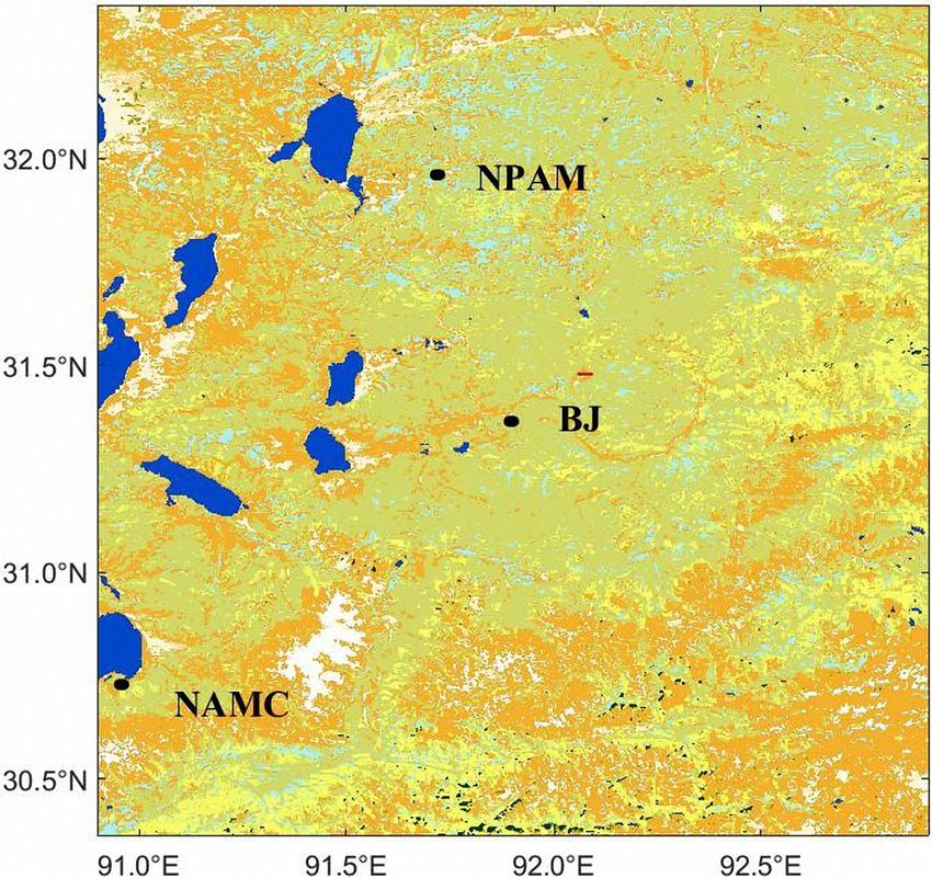
2916                             M. Li et al.: Variations in surface roughness of heterogeneous surfaces in the Nagqu area

a significant warming trend and increased precipitation (Li et     recent years, especially in the improvement of parameterisa-
al., 2010). The thermal effects of the Tibetan Plateau not only    tion schemes (Smirnova et al., 2016). Luo et al. (2009) used
have an important impact on the Asian monsoon and precip-          the land surface model CoLM to conduct a single-point nu-
itation variability but also affect the atmospheric circulation    merical simulation at the BJ station and successfully simu-
and climate in North America, Europe and the southern In-          lated the energy exchange process in the Nagqu area. Zhang
dian Ocean by inducing large-scale teleconnections similar         et al. (2017) evaluated the surface physical process param-
to the Asian–Pacific Oscillation (Zhou et al., 2009).              eterisation schemes of the Noah LSM (land surface model)
   The various thermal and dynamic effects of the Tibetan          and Noah-MP (multi-parameterisation) model in the entire
Plateau on the atmosphere affect the free atmosphere via the       East Asia region and evaluated the simulation of the surface
atmospheric boundary layer. Therefore, it is particularly im-      heat flux of the Tibetan Plateau. Xie et al. (2017) explored
portant to analyse the micrometeorological characteristics of      the simulation effect of the land surface model CLM4.5 in
the atmospheric boundary layer of the Tibetan Plateau, espe-       the alpine meadow area of the Qinghai-Tibet Plateau. Xu
cially the near-surface layer (Li et al., 2000). Affected by the   et al. (2018) studied the applicability of different parame-
unique underlying surface conditions of the Tibetan Plateau,       terisation schemes in the Weather Research and Forecast-
local heating shows interannual and interdecadal variability       ing (WRF) model when simulating boundary layer charac-
(Zhou et al., 2009). Different underlying surfaces have differ-    teristics in the Nagqu area. Comparative analyses have been
ing diversities, complex compositions and uneven distribu-         performed of the meteorological elements simulated by dif-
tions, which also makes the land surface that they constitute      ferent land surface process schemes in the WRF model in the
diverse and has a certain degree of complexity. As the main        Yellow River source region (Zhang et al., 2020). However,
input factor for atmospheric energy, the surface greatly af-       the applicability of the model in the Tibetan Plateau needs
fects the various interactions between the ground and the at-      further study. The terrain of the Tibetan Plateau is complex,
mosphere and even plays a key role in local areas or specific      the underlying surface is very uneven and the area has high
times (Guan et al., 2009). The surface characteristic param-       spatial heterogeneity. Because the condition of the underly-
eters (dynamic roughness, thermodynamic roughness, etc.)           ing surface has a very significant impact on the surface flux,
play an important role in the land surface process and are im-     obtaining information on the surface vegetation status of a
portant factors in causing climate change (Jia et al., 2000).      certain area is very helpful for analysing the spatial represen-
The underlying surface of the Tibetan Plateau presents dif-        tation of the surface flux.
ferent degrees of fluctuation, which introduces certain ob-           In this study, satellite data were obtained by MODerate-
stacles to understanding the land–atmosphere interaction of        resolution Imaging Spectroradiometer (MODIS), and the
the Tibetan Plateau. The fluctuating surface may alter the ar-     normalised difference vegetation index (NDVI) in the Nagqu
rangement of roughness elements on the surface and cause           area was used to study the dynamic surface roughness length.
changes in surface roughness. Changes in roughness can also        Atmospheric turbulence observation data in 2008, 2010
affect changes in the characteristics of other surface turbulent   and 2012 and observation data from automatic weather sta-
transportation, which may also result in changes in surface        tions were collected at three observation stations. The mea-
fluxes. Chen et al. (2015) presented a practical approach for      sured values of the average wind speed and turbulent flux
determining the aerodynamic roughness length at fine tempo-        of a single-height ultrasonic anemometer were used to deter-
ral and spatial resolutions over the landscape by combining        mine the surface dynamic roughness Z0 m (Chen et al., 1993).
remote-sensing and ground measurements. Surface rough-             The timescale dynamics of Z0 m and the results of different
ness is an important parameter in land surface models and          underlying surfaces were analysed. Through a comparison
climate models. Its size controls the exchange, transmission       of the calculation results to the observation data, we stud-
intensity and interactions between the near-surface airflow        ied whether the surface roughness values retrieved by satel-
and the underlying surface to some extent (Liu et al., 2007;       lites were reliable to provide accurate surface characteristic
Irannejad and Shao, 1998; Shao, 2000; Zhang and Lv, 2003).         parameters. Then we used the retrieved surface roughness
Zhou et al. (2012) demonstrated that simulated sensible heat       to replace the surface roughness in the original model for
flux compared with measurement was significantly improved          numerical simulation experiments, and evaluated the model
using a time-dependent Z0 m parameter. Therefore, the pri-         simulation results. This research will be helpful for the study
mary objective of this study is to calculate the surface rough-    of land–atmosphere interactions in the plateau area and im-
ness and its variation characteristics to further understand the   provement of the theoretical research of the near-surface
land–atmosphere interactions on the central Tibetan Plateau.       layer on the Tibetan Plateau. In the following section, we de-
   Through the study of surface roughness, it is beneficial to     scribe the case study area, the MODIS remote-sensing data,
obtain the land surface characteristics in the region, provide     the ground observations and the land cover map used to drive
the ground truth value for model inputs, improve land sur-         the revised Massman model (Massman, 1997; Massman and
face simulations in the Tibetan Plateau and deepen the un-         Weil, 1999). In Sect. 3, we present the results and then a vali-
derstanding of land–atmosphere interaction processes. Sim-         dation based on flux measurements at Nagqu station. Finally,
ulation of surface fluxes has made considerable progress in        we provide some concluding remarks on the variation char-

Hydrol. Earth Syst. Sci., 25, 2915–2930, 2021                                       https://doi.org/10.5194/hess-25-2915-2021
M. Li et al.: Variations in surface roughness of heterogeneous surfaces in the Nagqu area                                      2917

                                                                      ultrasonic wind thermometer and humidity probe pulsator
                                                                      and includes data on temperature and humidity, air pressure,
                                                                      average wind speed, average wind direction, surface radia-
                                                                      tive temperature, soil heat flux, soil moisture and temperature
                                                                      and radiation (Ma et al., 2006). The NAMC station is located
                                                                      at 30◦ 46.440 N, 90◦ 59.310 E and has an altitude of 4730 m.
                                                                      It is located on the southeastern shore of Nam Co lake in
                                                                      Namuqin Township, Dangxiong County, Tibet Autonomous
                                                                      Region. It is backed by the Nyainqêntanglha mountain range,
                                                                      and the underlying surface is an alpine meadow. This study
                                                                      uses NPAM station data for the whole year of 2012 and
                                                                      NAMC station data for the whole year of 2010.
                                                                         The land cover data used in this study are GLC2009 (Arino
                                                                      et al., 2010) data from the Envisat satellite in 2009, and the
Figure 1. Location of sites and the land cover on the northern Ti-    spatial resolution is 300 m. The classification standard is the
betan Plateau. The black solid circle “•” indicates the location of   land cover classification system (LCCS), and it divides the
the sites.                                                            global surface into 23 different types, with the study area in-
                                                                      cluding 14 of these types. The actual situation in the selected
                                                                      area does not match the data part of GLC2009 because of
acteristics of aerodynamic roughness lengths and numerical            the lack of an underlying surface, such as farmland, in the
simulation of the surface turbulent flux in the Nagqu area of         selected area. Therefore, according to the actual land cover
the central Tibetan Plateau.                                          types obtained by Chu et al. (2010), the categories irrigated
                                                                      farmland, dry farmland, mixed farmland vegetation, mixed
                                                                      multi-vegetation land, closed grassland and open grassland
2     Study area, data and methods                                    are replaced with six grasslands, shrub meadows, mountain
                                                                      meadows, alpine grasslands, alpine meadows and sparse veg-
2.1    Study area and data                                            etation in the mountains. Since the proportion of the un-
                                                                      derlying surface of the tree as a whole is only 0.36 %, the
The area selected in this study is a 200×200 km2 area centred         underlying surface types evergreen coniferous forest, mixed
on the Nagqu Station of Plateau Climate and Environment of            forest, multi-forest grassland mix and multi-grass forestland
the Northwest Institute of Ecology and Environmental Re-              mix will no longer be studied.
sources, Chinese Academy of Sciences.                                    The MODerate-resolution Imaging Spectroradiome-
   In this area, three meteorological observatory stations are        ter (MODIS) is a sensor on board the satellites TERRA
located: North Pam (Portable Automated Meso-net) Auto-                and AQUA launched by the US Earth Observing System
matic Meteorological Observatory (NPAM), Nam Co Sta-                  Program. The band of the MODIS sensor covers the full
tion for Multisphere Observation and Research, Chinese                spectrum from visible light to thermal infrared; thus, this
Academy of Sciences (NAMC) and BJ station (Fig. 1). The               sensor can detect surface and atmospheric conditions,
underlying surface around the observation site is relatively          such as surface temperature, surface vegetation cover,
flat on a small spatial scale, and a certain undulation is ob-        atmospheric precipitation and cloud top temperature. The
served at a large spatial scale. The data used included obser-        finest spatial resolution is 250 m. The normalised vegetation
vations from atmospheric turbulence and automatic meteoro-            index obtained by MODIS is the MYD13Q1 product, which
logical stations.                                                     provides a global resolution of 250 m per 16 d. This study
   The BJ station is located at coordinates 31.37◦ N, 91.90◦ E        selects 73 data files for 2008, 2010 and 2012 in Nagqu.
and has an altitude of 4509 m a.s.l. The BJ observation site
is located in the seasonal frozen soil area, and the vegeta-          2.2     Methodology
tion is alpine grassland. The site measurement equipment in-
cludes an ultrasonic anemometer (CAST3, Campbell, Inc.),              2.2.1    Method for calculating surface roughness by
CO2 /H2 O infrared open path analyser (LI 7500), and an au-                    observation data
tomatic meteorological observation system (Ma et al., 2006).
                                                                      Using the measured values of the average wind speed and
This study uses the BJ station data from 2008 and 2012. The
                                                                      turbulent flux of a single-height ultrasonic anemometer, the
NPAM station is located at 31◦ 560 N, 91◦ 430 E and has an
                                                                      calculation scheme of surface roughness proposed by Chen
altitude of approximately 4700 m. The ground of the experi-
                                                                      et al. (1993) was selected, and the dynamic variation in the
mental field is flat, and the area is wide. The ground is cov-
                                                                      surface roughness was obtained.
ered by a plateau meadow that grows 15 cm high in summer.
The experimental station observation equipment includes an

https://doi.org/10.5194/hess-25-2915-2021                                          Hydrol. Earth Syst. Sci., 25, 2915–2930, 2021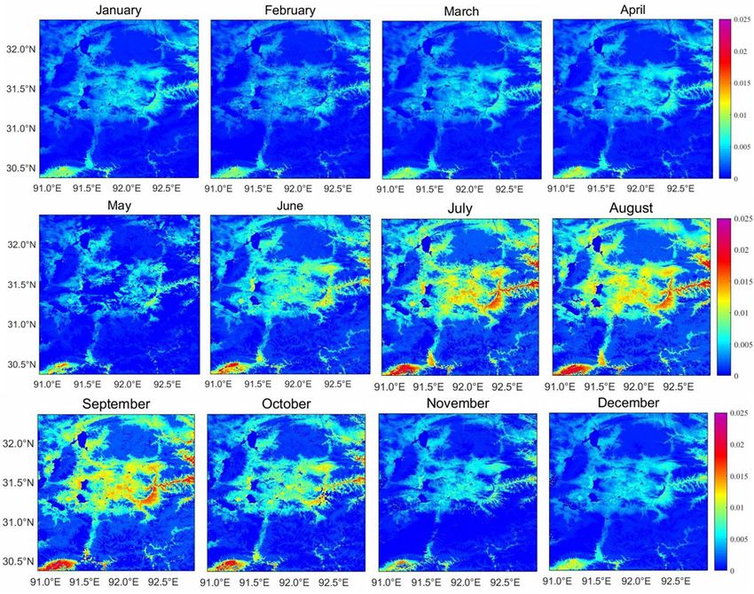
2918 M. Li et al.: Variations in surface roughness of heterogeneous surfaces in the Nagqu area
According to the Monin–Obukhov similarity theory
(Monin and Obhukov, 1954), the wind profile formula with
γ = C1 − C2 · exp (−C3 · Cd · LAI) (5)
the stratification stability correction function (Panosky and
Dutton, 1984) is as follows: Cd · LAI
nec = (6)
2·γ2
u∗ z−d
1 − exp (−2 · nec )
U (z) = ln − ψm (ζ ) (1) dh = 1 − (7)
k Z0 m 2 · nec
1 + x2
1+x π Z0 m
k
ψm(ζ ) =2 ln + ln − tan−1 (x) + = [1 − dh ] · exp − , (8)
2 2 2 h γ
ζ 0, (3) the model and related to the surface drag coefficient; LAI is
p the leaf area index; Cd = 0.2 is the drag coefficient of the
where u∗ = −u0 w0 ; Z0 m is the dynamic surface roughness foliage elements; nec is the wind speed profile coefficient of
length; z is the height of wind observation; d is zero plane fluctuation in the vegetation canopy; and h is the vegetation
displacement, d = 2/3h (Stanhill, 1969), h is the vegetation height. In many earlier studies, the high-altitude environment
height. h takes 0 in winter, 0.020 in spring, 0.0450 in sum- of the Tibetan Plateau was correlated with a low temperature
mer and 0.030 in autumn in this study; U is the average in the study area and shown to affect the height and sparse-
wind speed; k is the Karman constant, which is set to 0.40 ness of the vegetation. Based on previous research, this study
u3∗
(Högström, 1996); L = − is the Monin–Obukhov considers that the vegetation height in northern Tibet is re-
(k g )θ 0 ω0
θ lated to the normalised difference vegetation index (NDVI)
length (Monin and Obhukov, 1954); x = (1 − 16ζ )1/4 ; and and altitude (Chen et al., 2013) and introduces the altitude
ζ = (z − d)/L is the atmospheric stability parameter. Avail- correction factor on the original basis. The following is the
able from Eq. (1), calculation formula:
z−d kU
hmax − hmin
ln = + ψm (ζ ). (4) H = hmin + (NDVI − NDVImin ) (9)
Z0 m u∗ NDVImax − NDVImin
Using Eq. (2)–(4), Z0 m can be determined by fitting ζ and h = acf · H , (10)
observing a single height kU
u∗ . where hmin and hmax are the minimum and maximum veg-
2.2.2 Method for calculating surface roughness by etation height observed at the observation station, respec-
satellite data tively, NDVImax and NDVImin are the maximum and min-
imum NDVI of the observation station, respectively; H is
For a fully covered uniform canopy, Brutsaert (1982) sug- based on the assumption that the vegetation height is directly
gested that Z0 m = 0.13hv. For a canopy with proportional proportional to the NDVI; x is the altitude, which is obtained
coverage (partial coverage), Raupach (1994) indicated that from ASTER’s digital elevation model (DEM) products; and
Z0 m varies with the leaf area index (LAI). However, Pierce et acf is the altitude correction factor (Chen et al., 2013), which
al. (1992) pointed out that for all kinds of biological groups, is used to characterise the effect of elevation on the height
the leaf area index can be obtained from the NDVI, and the of vegetation in northern Tibet. The acf parameter has the
fractional cover of vegetation can be related to the NDVI. following form:
Asrar et al. (1992) pointed out that a mutual relationship oc-
curred among the LAI, NDVI and ground cover through the 0.149, x > 4800
acf = 11.809 − 0.0024 · x, 4300 < x < 4800 . (11)
study of physical models. The study by Moran et al. (1994)
1.49, x < 4300
provides another method that uses the function of the rela-
tionship between NDVI and Z0 m in the growing season of The LAI used in this study is calculated by the NDVI of
alfalfa. MODIS (Su, 1996). The calculation formula is as follows:
Considering that the main underlying surface of the study
area is grassland, this study selects the Massman model 0.5
NDVI · (1 + NDVI)
(Massman, 1997; Massman and Weil, 1999). to calculate the LAI = . (12)
1 − NDVI
Z0 m in the Nagqu area of the central Tibetan Plateau. The
Massman model is calculated as follows:
Hydrol. Earth Syst. Sci., 25, 2915–2930, 2021 https://doi.org/10.5194/hess-25-2915-2021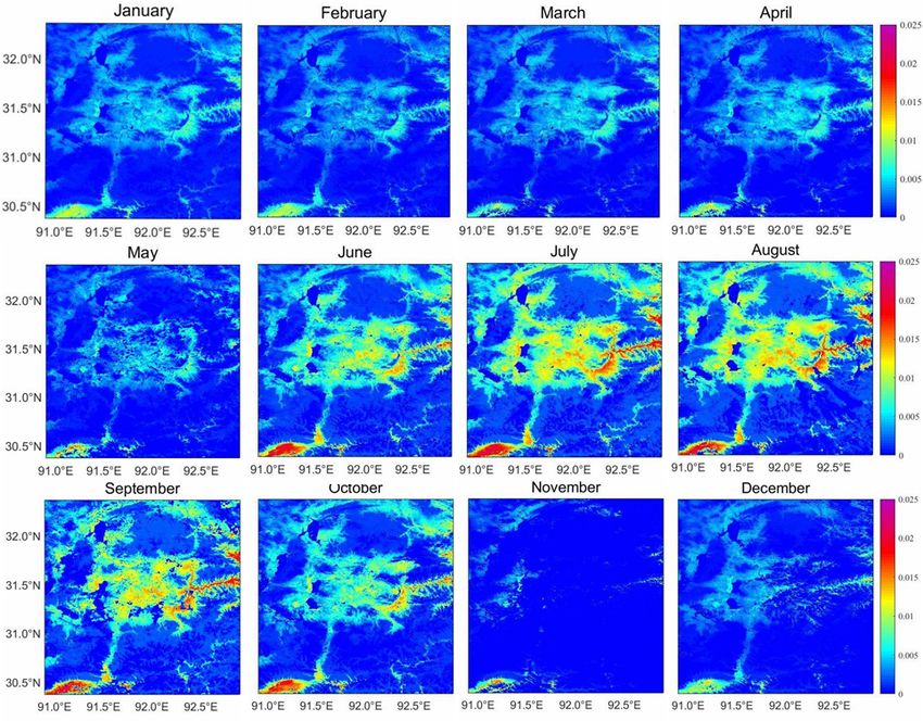
M. Li et al.: Variations in surface roughness of heterogeneous surfaces in the Nagqu area 2919
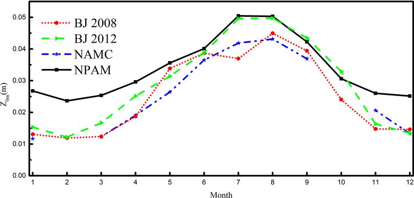
Figure 2. Surface roughness length of different sites on the northern Tibetan Plateau.
3 Results analysis crease in precipitation that accelerated the growth of vegeta-
tion and the rapid rise of Z0 m . In June, July and August, con-
3.1 Variation characteristics of surface roughness tinuous precipitation and rising temperatures led to vigorous
based on measured data vegetation growth, although changes were not observed af-
ter the vegetation reached maturity. The corresponding max-
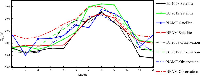
Figure 2 shows the temporal variation characteristics of the imum value of Z0 m in the figure remains unchanged, al-
surface roughness of sites in different years in the Nagqu though due to high values in these 3 months, the area with
area. The Z0 m value has continued to increase since Febru- high Z0 m values gradually expanded and reached the maxi-
ary to reach a maximum in July and August. The results for mum range in August. From September to December, as the
the BJ and NPAM stations in 2012 show that July has slightly plateau summer monsoon retreated, the temperature and hu-
larger ones than August, and the results for the NAMC sta- midity gradually decreased. Compared with the plateau sum-
tion in 2010 and BJ station in 2008 show that August has mer monsoon, the conditions were no longer suitable for veg-
larger values than July. After August, the Z0 m value began etation growth; thus, the contribution of vegetation to Z0 m
to decrease, and in December, the value was approximately was weakened, the surface vegetation height gradually de-
the same as the value in January. In general, the change in the creased and Z0 m continued to decrease. Moreover, the area
Z0 m degree of each station increases from spring to summer with high Z0 m value also gradually decreased.
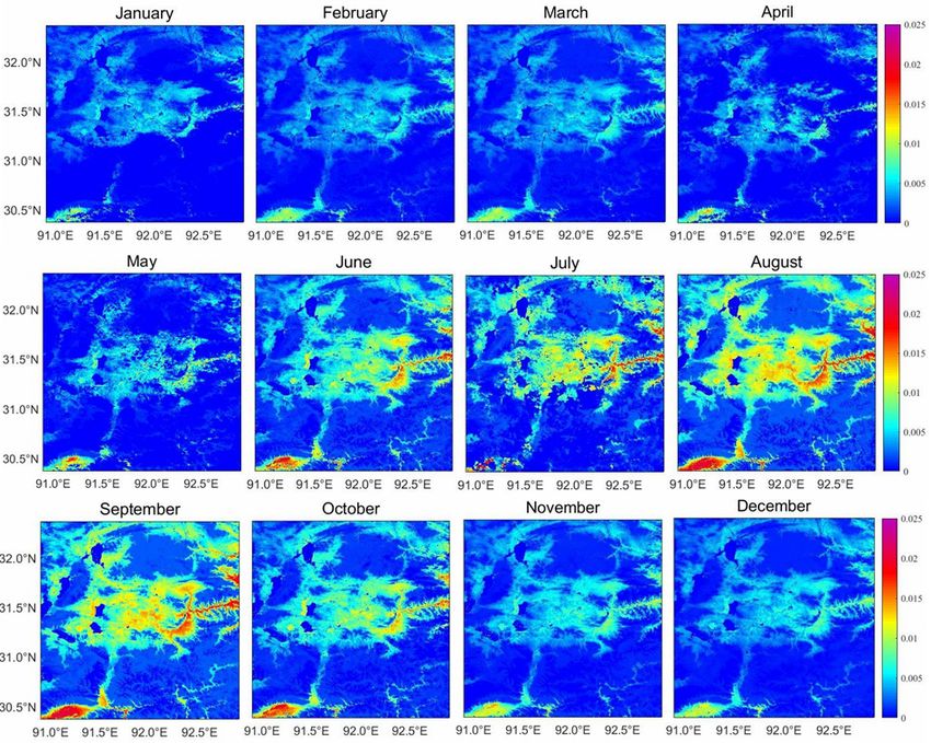
and decreases month by month from summer to winter. Figures 4 and 5 show the retrieved monthly surface rough-
ness values in the BJ area in 2010 and 2012, respectively.
3.2 Spatio-temporal variation characteristics of Moreover, Z0 m also showed a decrease from January to
surface roughness length retrieved by MODIS data February in the Nagqu area in 2010 and 2012. Starting in
February, Z0 m increased. Starting in June, Z0 m increased
Figure 3 shows a plot of the surface roughness distribution
rapidly and reached the peak of the whole year in August.
of 200 × 200 km2 around the BJ site in 2008. In February,
Subsequently, Z0 m began to decrease.
the Z0 m decreased from January, which may have been due
Figures 3–5 show that Z0 m changes with the spatial and
to snowfall or temperature, etc., resulting in a small Z0 m
temporal scale. Z0 m shows different trends on different un-
that continued to decrease. Due to the rising temperature and
derlying surfaces. In November 2008, the Z0 m in the Nagqu
snow melting, Z0 m showed a slowly increasing trend from
area was small overall and generally as low as 1 cm. His-
February to May and a rapid increase from June to August.
torical data show that there is a large-scale snowfall process
From June onwards, a large number of surface textures were
in the Nagqu area at this time. Snowfall over the meadow
observed, indicating the complexity of the underlying sur-
causes the underlying surface of the meadow to be homoge-
face. Whether the bulk surface or vegetation had a more im-
neous and flat, and after the snowfall falls, it is easy to form
portant impact on Z0 m is not clear. From May to August, ob-
a block with a scattered and discontinuous underlying sur-
vious changes in humidity, temperature and pressure caused
face. We subsequently determined that the surface roughness
by the plateau summer monsoon led to an increase in the
of the area with ice and snow as the underlying surface is not
height and coverage of surface vegetation, and Z0 m peaked
more than 1 cm, which is consistent with historical weather
in August. In particular, the change from May to June was
processes. Therefore, we think that snowfall caused the Z0 m
very significant, which may have been related to the begin-
in November to be very small. From November to Decem-
ning of the summer monsoon in June, the corresponding in-
https://doi.org/10.5194/hess-25-2915-2021 Hydrol. Earth Syst. Sci., 25, 2915–2930, 2021
2920                              M. Li et al.: Variations in surface roughness of heterogeneous surfaces in the Nagqu area

Figure 3. Surface roughness length on the northern Tibetan Plateau in 2008.

ber, Z0 m showed a growing trend, which may be due to tem-             were larger than the satellite-data-retrieved results through-
perature, unfrozen soil or other reasons that resulted in the          out the year. The calculation results of the site data were
melting of snow, and then the surface roughness showed a               very close to the satellite-data-retrieved results from January
growing trend (Zhou et al., 2017).                                     to April and July to November, although a large difference
                                                                       was observed in May, June and December, with the largest
3.3    Evaluation of satellite-data-retrieved results                  difference occurring in May at 1.8 cm. In 2012, the BJ site
                                                                       data calculation results were consistent with the satellite-
                                                                       data-retrieved results for the whole year, although the site
The underlying surfaces of the three sites selected in this
                                                                       data calculation results were larger than the satellite-data-
study are all alpine meadows. In Fig. 6, the NPAM site data
                                                                       retrieved results from March to June, and the station data cal-
calculation results are larger than the satellite-data-retrieved
                                                                       culation results were smaller than the satellite-data-retrieved
results throughout the year. Only the values in September
                                                                       at other times. As a result, the largest difference occurred in
and October are very close, and the trends are similar. The
                                                                       June at 1.1 cm. Figure 6 shows that for the overall situation,
maximum value of the site data calculation is 5 cm, and the
                                                                       the seasonal variation trend of the site data calculation results
satellite-data-retrieved result is 4.5 cm. The maximum dif-
                                                                       is consistent with the satellite-data-retrieved results in Jan-
ference is in May at 1.7 cm. The NAMC station data cal-
                                                                       uary, February, March, November and December. However,
culation results are very close to the satellite-data-retrieved
                                                                       the site data calculation results from April to October are
results from April to November, although the satellite-data-
                                                                       greater than the satellite-data-retrieved results. From Fig. 6,
retrieved results are significantly larger than the site data cal-
                                                                       the Z0 m calculated from the site observation data is larger
culation results in January, March and December. The largest
                                                                       than that of the satellite data, which may be because of the
difference occurs in January, and the difference value reaches
                                                                       average smoothing effect. From February to July, the single-
1.5 cm. In 2008, the calculation results of the BJ station data

Hydrol. Earth Syst. Sci., 25, 2915–2930, 2021                                           https://doi.org/10.5194/hess-25-2915-2021
M. Li et al.: Variations in surface roughness of heterogeneous surfaces in the Nagqu area                                        2921

Figure 4. Surface roughness length on the northern Tibetan Plateau in 2010.

point Z0 m value was significantly increased according to the          age results of the underlying surface is 0.83, and the corre-
independent method of determining the surface roughness,               lation coefficient with the satellite-retrieved results is 0.62.
while the results obtained using the satellite data did not in-        Because the NAMC observation station is closer to the lake
crease significantly. The satellite results show that the values       (1 km), it is more affected by local microclimates, such as
from January to May, November and December are basically               lake and land winds. The results in Fig. 7 all passed the
stable below 2 cm and only change from June to October,                F test of P = 0.05, which indicates that there is no signif-
which is related to non-uniformity of the underlying surface           icant difference between the site data calculation results and
in Massman model. In general, the results calculated by the            the satellite-data-retrieved results.
station are generally larger than those obtained by satellite
retrieval.
   The Z0 m scatter plot is shown in Fig. 7. A significant posi-       4      Variation characteristics of the surface roughness of
tive correlation is observed between the satellite retrieval and              different underlying surfaces
the surface roughness calculated from the site data. The cor-
                                                                       According to the vegetation dataset GLC2009, combined
relation coefficients between the observation result and the
                                                                       with actual local conditions, the 200×200 km2 area of Nagqu
retrieved result are large, except for at the NAMC station
                                                                       was divided into 10 different underlying surfaces (Arino
in 2010 in Fig. 7g. The average results of the underlying sur-
                                                                       et al., 2010): mountain grassland, shrub meadow, mountain
face were consistent with the underlying surface results in
                                                                       meadow, alpine grasslands, alpine meadows, sparse vegeta-
different regions, further indicating that the satellite-retrieved
                                                                       tion lap, urban land, bare land, water bodies, ice sheets and
results are consistent with the site calculation results. How-
                                                                       snow cover.
ever, the results of the NAMC site are different from those
of the other sites. The correlation coefficient with the aver-

https://doi.org/10.5194/hess-25-2915-2021                                             Hydrol. Earth Syst. Sci., 25, 2915–2930, 2021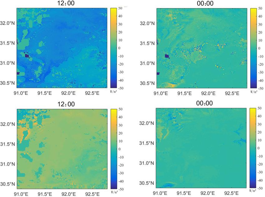
2922                              M. Li et al.: Variations in surface roughness of heterogeneous surfaces in the Nagqu area

Figure 5. Surface roughness length on the northern Tibetan Plateau in 2012.

Figure 6. Comparison of the surface roughness length by site observations and satellite-remote-sensing-retrieved data.

   The monthly variation in Z0 m in different underlying sur-           than that of other types throughout the year, and the change
faces in the Nagqu area is shown in Fig. 8, which indicates             in Z0 m is very large, which is probably due to the irregular
that 14 different underlying surfaces (Table 1) in the Nagqu            changes in the underground areas of the selected areas and
area can be divided into four categories. The first category            the irregularities caused by human activities. The second cat-
is urban land, which accounts for 0.07 % of the whole study             egory is lush grassland, including shrub meadows, mountain
area. The Z0 m of this type of underlying surface is greater            grasslands, alpine grasslands and mountain meadows, which

Hydrol. Earth Syst. Sci., 25, 2915–2930, 2021                                             https://doi.org/10.5194/hess-25-2915-2021
M. Li et al.: Variations in surface roughness of heterogeneous surfaces in the Nagqu area                                        2923

Figure 7. Scatter plots of the retrieved and calculated surface roughness lengths at four sites.

https://doi.org/10.5194/hess-25-2915-2021                                                Hydrol. Earth Syst. Sci., 25, 2915–2930, 2021
2924                               M. Li et al.: Variations in surface roughness of heterogeneous surfaces in the Nagqu area

Figure 8. Curve of the surface roughness length for different underlying surfaces.

Hydrol. Earth Syst. Sci., 25, 2915–2930, 2021                                        https://doi.org/10.5194/hess-25-2915-2021
M. Li et al.: Variations in surface roughness of heterogeneous surfaces in the Nagqu area                                 2925

Table 1. Legend of the land cover map on the northern Tibetan     and begins to increase after February, reaching a peak in Au-
Plateau.                                                          gust and then starting to decrease. However, Fig. 6 clearly
                                                                  shows that there are several stages in which Z0 m changes
                                                                  significantly, in early April, mid-May, early July, late Au-
                                                                  gust and late September. The change at the end of August
                                                                  was the most obvious. At each of the underlying surfaces,
                                                                  Z0 m changes by more than 2 cm on average. The extent of
                                                                  the change in late September was also large, with an average
                                                                  change of more than 1.5 cm. Moreover, the change in early
                                                                  July was special because the change resulted in a significant
                                                                  increase in the Z0 m of water bodies and ice.
                                                                     Certain factors, such as cloud cover in May, August and
                                                                  November 2008, August and September 2010, and April and
                                                                  July 2012, caused significant changes in the overall Z0 m ,
                                                                  which resulted in two very significant changes in the 3-year
                                                                  average for August and November. In November, the change
                                                                  was caused by snowfall based on other meteorological data.
                                                                  In August 2008 and 2010, the changes were caused by pre-
                                                                  cipitation based on an analysis of the sudden increase in
                                                                  the Z0 m of the water body and ice and snow surface. Com-
                                                                  bined with several changes in Z0 m , precipitation, snowfall
accounts for 62.49 % of the area. The variation curves of Z0 m    and snow accumulation will make the underlying surface
of the four underlying surfaces are similar, and the Z0 m of      more uniform and flatter, which will lead to relative reduc-
the urban land is only smaller than that of other underly-        tions in Z0 m .
ing surfaces. The third category is sparse grassland, includ-
ing alpine sparse vegetation, alpine meadows and bare land,
and it accounts for 33.74 % of the area. The Z0 m values of       5     Simulation and evaluation of the impact of surface
the three underlying surfaces are similar at a medium height.           roughness on turbulent fluxes using the Noah-MP
The Z0 m of the bare soil is at the lowest point of these un-           model
derlying surface Z0 m , and the Z0 m of the alpine meadow is
                                                                  5.1    Model setup
relatively stable and less affected by the outside vegetation.
The fourth category is ice and snow, including ice surfaces       According to the surface roughness variation characteristics
and snow cover and water bodies, which are two kinds of           retrieved from satellite data, the underlying surface of Nagqu
underlying surfaces, accounting for 3.7 % of the area. The        area can be divided into four types. They are urban, lush
Z0 m of these three underlying surfaces presents another phe-     grass, sparse grass and ice and snow. Among them, urban
nomenon. The variation range of the whole year is relatively      accounts for 0.07 %, and its Z0 m is up to 9 cm; lush grass-
small, and the Z0 m of these underlying surfaces is also small.   land accounts for 62.49 % of the area, and its Z0 m can reach
It is more than 1 cm in mid-June and less than 1 cm at other      up to 6 cm; sparse grassland accounts for up to 33.74 %, and
times. Figure 8d shows the multi-year average seasonal vari-      its Z0 m can reach up to about 4 cm; and ice and snow ac-
ation in Z0 m . The figure clearly shows that the underlying      counts for 3.7 % of the area, and the Z0 m does not exceed
surface can be divided into four categories due to the differ-    1 cm. These results are substituted into Noah-MP to replace
ence in surface roughness. The change from January to May         the original parameter design numerical simulation experi-
Z0 m is very small, peaking from May to August and then           ment. The model after replacing the surface roughness is set
down to the previous January to May level in November and         as a sensitivity experiment, and the original model is set as
December. The snowfall in November 2008 may have led to           a control experiment. The selection of other parameterisa-
the low level of November in Fig. 8d. Table 2 shows that the      tion schemes suitable for numerical simulation in the Nagqu
winter albedo at the BJ station and NAMC station is higher        area is shown in Table 3. The simulation time is from 1 to
than that in other seasons, and it is the smallest in the sum-    31 July 2008, and the spin-up time is 9 d. The forcing field
mer. The surface albedo at both stations in November 2008         dataset is a Chinese meteorological forcing dataset (He et
was significantly higher than that in November of the other 2     al., 2020), jointly developed by the Tibetan Plateau Data As-
years. In fact, the surface roughness in November should be       similation and Modelling Centre and the Institute of Tibetan
higher than that in December in former years.                     Plateau Research of the Chinese Academy of Sciences (ITP-
   Figure 8 also shows that in the Nagqu area, except for         CAS).
the area of the fourth type of underlying surface, the Z0 m
change in other areas decreases from January to February

https://doi.org/10.5194/hess-25-2915-2021                                       Hydrol. Earth Syst. Sci., 25, 2915–2930, 2021
2926 M. Li et al.: Variations in surface roughness of heterogeneous surfaces in the Nagqu area
Table 2. The observed albedo of the sites (BJ and NAMC) on the northern Tibetan Plateau.
Site Year Jan Feb Mar Apr May Jun Jul Aug Sep Oct Nov Dec
2008 0.13 0.17 0.14 0.13 0.12 0.10 0.09 0.09 0.09 0.16 0.32 0.16
BJ 2009 0.30 0.26 0.30 0.25 0.26 0.21 0.19 0.19 0.21 0.26 0.24 0.26
2010 0.26 0.30 0.31 0.30 0.34 0.22 0.19 0.18 0.18 0.35 0.26 0.27
2008 0.28 0.28 0.31 0.28 0.25 0.21 0.17 0.18 0.18 0.30 0.89 0.28
NAMC 2009 0.35 0.32 0.28 0.24 0.26 0.22 0.19 0.17 0.22 0.24 0.31 0.27
2010 0.45 0.23 0.25 0.24 0.29 0.22 0.20 0.17 0.18 0.40 0.35 0.24
Table 3. The selected other schemes in Noah-MP.
Options for different schemes Name of the option
Dynamic vegetation Use table LAI; use FVEG = SHDFAC from input
Canopy stomatal resistance Ball–Berry method
Soil moisture factor for stomatal resistance Noah’s method
Runoff and groundwater TOPMODEL with groundwater
Surface layer drag coeff. Monin–Obukhov method
Supercooled liquid water No iteration
Frozen soil permeability Non-linear effects, less permeable
Radiation transfer Two-stream applied to grid cell
Ground snow surface albedo Classic method
Partitioning precipitation into rainfall and snowfall Jordan method
Lower boundary condition of soil temperature TBOT at ZBOT (8 m) read from a file
Snow/soil temperature time scheme Full implicit (original Noah); temperature top boundary condition
5.2 Evaluation of the simulated single-point heat flux are better than the control experiments, while latent heat flux
in the sensitivity experiment is greater than that in the control
experiment and is close to the observation results at NPAM
Figure 9a shows that the sensible heat flux simulated by the
site (Fig. 9f). It also shows that improving the accuracy of
sensitivity experiment is closer to the measured value than
surface roughness can improve the simulation effect of latent
the control experiment at the BJ site. In the daytime, the re-
heat flux.
sults of sensitivity experiment were in general smaller than
those of the control experiment. At night, the results of the
two models were close to each other before 21 July, and the 5.3 Evaluation of regional heat flux simulation results
sensitivity experiment results were significantly improved af-
ter 21 July. Figure 9b shows that the sensitivity experiment In order to compare the changes of sensible heat flux and la-
results are basically consistent with the control experiment tent heat flux before and after improvement, the sensitivity
results at the BJ site, which are maintained at about 0 W m−2 , simulations are used to subtract the control model simulation
and there is no improvement at night. Before 19 July, the la- results. By subtracting the sensible heat flux of control from
tent hear fluxes for the two experiments remained at about sensitivity experiment, the results are shown in Fig. 10. It can
200 W m−2 , which was less than the observed latent heat also be seen from Fig. 10a that the difference of sensible heat
flux, and the simulated maximum value of the sensitivity ex- flux is basically negative in the daytime, indicating that the
periment was greater than that of the control experiment. Af- sensible heat flux after improvement is smaller than that be-
ter 19 July, the two experiments simulation results began to fore improvement. The above results show that the modified
increase and reached about 400 W m−2 , consistent with the surface roughness can improve the simulation effect of sensi-
observed latent heat flux, indicating that the simulation ef- ble heat flux in daytime. The results in Fig. 10c are basically
fect was improved to some extent. Similarly, it can be found positive in the daytime, indicating that the latent heat flux
from the maximum value that the sensitivity experiment re- after improvement is larger than that before improvement,
sults were slightly greater than the control experiment re- about 15 W m−2 . The above results show that the model sim-
sults. The simulated values of sensible heat fluxes at NAMC ulation results are generally less than the actual observation
and NPAM sites (Fig. 9c and e) are significantly larger than results, so it can be considered that the improvement of sur-
the observation results, but the sensitivity experiment results face roughness in the daytime can improve the simulation of
Hydrol. Earth Syst. Sci., 25, 2915–2930, 2021 https://doi.org/10.5194/hess-25-2915-2021M. Li et al.: Variations in surface roughness of heterogeneous surfaces in the Nagqu area 2927
Figure 9. Comparison of simulated and observed sensible heat flux (a, c, e) and latent heat flux (b, d, f) at BJ, NAMC and NPAM sites.
heat fluxes. Figure 10 also shows that the improvement of A strong connection is observed between the monthly
night-time latent heat flux is not significant, which is basi- variation in surface roughness and the changes in me-
cally maintained at 0 W m−2 . teorological elements brought by the plateau summer
monsoon. Among them, the satellite surface retrieval
results in a slow increase in surface roughness from
6 Conclusions and discussion February to May.
Through the calculation and analysis of the surface rough- 2. Through the characteristics of surface roughness vari-
ness of the Nagqu area in the central Tibetan Plateau and ation retrieved by satellite data, the underlying surface
comparing the retrieved satellite data with the calculation re- can be divided into four categories according to the sur-
sults of the observational data, the main conclusions attained face roughness (from large to small): urban, lush grass-
are as follows. land, sparse grassland and ice and snow. Among them,
lush grassland accounts for 62.49 %, and the Z0 m can
1. The retrieved results of the satellite data are basically
reach 6 cm; sparse grassland accounts for 33.74 %, and
consistent with the calculated results of the measured
the Z0 m can reach up to 4 cm; and ice and snow ac-
data. Both results indicate that the surface roughness
counts for 3.7 %, and the Z0 m does not exceed 1 cm.
continued to increase from February to August, began
to decrease after reaching a peak in August and reached 3. Comparing satellite-retrieved results and measured data
the lowest value in February of the following year. shows that the results are positively correlated, and the
https://doi.org/10.5194/hess-25-2915-2021 Hydrol. Earth Syst. Sci., 25, 2915–2930, 20212928 M. Li et al.: Variations in surface roughness of heterogeneous surfaces in the Nagqu area
Figure 10. The difference of the control and sensitivity experiments simulated regional sensible heat flux at (a) 12:00 LT and (b) 00:00 LT
and latent heat flux at (c) 12:00 LT and (d) 00:00 LT.
satellite-retrieved results fit the measured results better. Code availability. The surface roughness length
Due to the average sliding effect of the retrieved data, code used in this article is available online at
the satellite-retrieved data are smaller than the measured https://doi.org/10.5281/zenodo.4797701 (Li and Liu, 2021).
results. This method can be used to calculate the surface
roughness results for a region and provide a true value
for the model for simulation. Data availability. The surface energy fluxes data
used in this article are available online at
4. The accuracy of ground–air flux simulation can be https://doi.org/10.11888/Meteoro.tpdc.270910 (Ma, 2020).
improved after adjusting the surface roughness in the
Nagqu area. After replacing the model surface rough-
ness, the sensible heat flux has improved by 20 W m−2 Author contributions. ML, XL, LS and YY mainly wrote the
during the daytime. The improvement for the simulation manuscript and were responsible for the research design, data
of sensible heat flux is poor at night, about 0.15 W m−2 . preparation and analysis. YM and ML supervised the research, in-
The improvement of latent heat flux is not obvious, and cluding methodology development, as well as manuscript structure,
writing and revision. ML drafted the manuscript. FS, SY, LW and
there is an improvement within 15 W m−2 during the
WF prepared the data and wrote this paper.
daytime.
This study uses remote-sensing images and an aerody-
namic roughness remote-sensing-retrieved model to estimate Competing interests. The authors declare that they have no conflict
the spatial scale of aerodynamic roughness conditions in of interest.
northern Tibet, and this method will provide parameter and
parameterisation scheme improvements for model simula-
tions to study the spatial distribution of the surface flux Special issue statement. This article is part of the special issue
“Data acquisition and modelling of hydrological, hydrogeological
in the Tibetan Plateau. Air thermodynamics surface rough-
and ecohydrological processes in arid and semi-arid regions”. It is
ness (Z0 h ) is affected by shortwave and longwave radiation
not associated with a conference.
(the latter for deriving surface temperature), air temperature,
wind speed, precipitation and snowfall. The relationship be-
tween air thermodynamics surface roughness and these other Acknowledgements. This work was financially supported by the
variables and how to parameterise them in the Massman Second Tibetan Plateau Scientific Expedition and Research (STEP)
model will be studied in the future.
Hydrol. Earth Syst. Sci., 25, 2915–2930, 2021 https://doi.org/10.5194/hess-25-2915-2021M. Li et al.: Variations in surface roughness of heterogeneous surfaces in the Nagqu area 2929
program (grant no. 2019QZKK0103), the National Natural Sci- Irannejad, P. and Shao, Y. P.: Description and validation of
ence Foundation of China (grant nos. 41675106 and 41805009), the atmosphere-land-surface interaction scheme (ALSIS) with
the National Key Research and Development Program of HAPEX and Cabauw data, Global Planet. Change, 19, 87–114,
China (grant no. 2017YFC1505702) and the Scientific Research https://doi.org/10.1016/S0921-8181(98)00043-5, 1998.
Project of Chengdu University of Information Technology (grant Jane, Q.: The third pole, Nature, 454, 393–396, 2008.
no. KYTZ201721). Jia, L.: The Characteristics of Roughness Length for Heat and Its
Influence on Determination of Sensible Heat Flux in Arid Zone,
Plateau Meteorol., 19, 495–503, 2000.
Financial support. This research has been supported by the Second Li, J. L., Hong, Z. X., and Sun, S. F.: An Observational Ex-
Tibetan Plateau Scientific Expedition and Research (STEP) pro- periment on the Atmospheric Boundary Layer in Gerze Area
gram (grant no. 2019QZKK0103). of the Tibetan Plateau, Chin. J. Atmos. Sci., 24, 301–312,
https://doi.org/10.1007/s10011-000-0335-3, 2000.
Li, L., Chen, X. G., Wang, Z. Y., Xu, W. X., and Tang,
Review statement. This paper was edited by Philip Brunner and re- H. Y.: Climate Change and Its Regional Differences over
viewed by three anonymous referees. the Tibetan Plateau, Adv. Clim. Change Res., 6, 181–186,
https://doi.org/10.3969/j.issn.1673-1719.2010.03.005, 2010.
Li, M., and Liu, X.: code_for calculate z0m in Matlab, Zenodo,
https://doi.org/10.5281/zenodo.4797701, 2021.
References Liu, J., Zhou, M., and Hu, Y.: Discussion on the Terrain Aerody-
namic Roughness, Ecol. Environ., 16, 1829–1836, 2007.
Arino, O., Ramos, J., Kalogirou, V., Defourny, P., and Achard, F.: Luo, S., Lü, S., and Yu, Z.: Development and validation of the
Glob Cover 2009, in: Proceedings of the living planet Sympo- frozen soil parameterization scheme in Common Land Model,
sium, Edinburgh, UK, 686–689, available at: http://hdl.handle. Cold Reg. Sci. Technol., 55, 130–140, 2009.
net/2078.1/74498 (last access: 18 February 2011), 2010. Ma, Y.: A long-term dataset of integrated land-
Asrar, G., Myneni, R. B., and Choudhury, B. J. : Spatial hetero- atmosphere interaction observations on the Tibetan
geneity in vegetation canopies and remote sensing of absorbed Plateau (2005–2016), National Tibetan Plateau Data Cen-
photosynthetically active radiation: A modelling study, Re- ter, https://doi.org/10.11888/Meteoro.tpdc.270910, 2020.
mote Sens. Environ., 41, 85–103, https://doi.org/10.1016/0034- Ma, Y. and Wang, J. M.: Analysis of Aerodynamic and Thermody-
4257(92)90070-Z, 1992. namic Parameters on the Grassy Marshland Surface of Tibetan
Brutsaert, W. A.: Evaporation into the Atmosphere, D. Reidel Plateau, Prog. Nat. Sci., 12, 36–40, 2002.
Publishing Company, Dordrecht, the Netherlands, 113–121, Ma, Y., Tsukamoto, O., Wang, J. M., Ishikawa, H., and Tamagawa,
https://doi.org/10.1007/978-94-017-1497-6, 1982. I.: Analysis of aerodynamic and thermodynamic parameters on
Chen, J., Wang, J., and Mitsuaki, H.: An independent method to the grassy marshland surface of Tibetan Plateau, Prog. Nat. Sci.,
determine the surface roughness length, Chin. J. Atmos. Sci., 12, 36–40, 2002.
17, 21–26, https://doi.org/10.3878/j.issn.1006-9895.1993.01.03, Ma, Y., Yao, T., Wang, J., and Hu, Z.: The Study on the Land Sur-
1993. face Heat Fluxes over Heterogeneous Landscape of the Tibetan
Chen, Q. T., Jia, L., Hutjes, R., and Menenti, M.: Estimation of Plateau, Adv. Earth Sci., 21, 1215–1223, 2006.
Aerodynamic Roughness Length over Oasis in the Heihe River Massman, W.: An analytical one-dimensional model of momentum
Basin by Utilizing Remote Sensing and Ground Data, Remote transfer by vegetation of arbitrary structure, Bound.-Lay. Me-
Sens., 7, 3690–3709, https://doi.org/10.3390/rs70403690, 2015. teorol., 83, 407–421, https://doi.org/10.1023/A:1000234813011,
Chen, X., Su, Z., Ma, Y., Yang, K., Wen, J., and Zhang, 1997.
Y.: An improvement of roughness height parameterization Massman, W. and Weil, J. C.: An analytical one-dimensional
of the Surface Energy Balance System (SEBS) over the second-order closure model of turbulence statistics and the
Tibetan Plateau, J. Appl. Meteorol. Clim., 52, 607–622, Lagrangian time scale within and above plant canopies
https://doi.org/10.1175/JAMC-D-12-056.1, 2013. of arbitrary structure, Bound.-Lay. Meteorol., 91, 81–107,
Chu, D., Basabta, S., Wang, W., Zhang, Y. L., Liu, L. S., and https://doi.org/10.1023/A:1001810204560, 1999.
Shushil, P.: Land Cover Mapping in the Tibet Plateau Using Monin, A. and Obukhov A.: Basic laws of turbulent mixing in the
MODIS Imagery, Resour. Sci., 32, 2152–2159, 2010. atmosphere near the ground, Tr. Akad. Nauk SSSR Geofiz. Inst.,
Guan, X. D., Huang, J. P., Guo, N., Bi, J. R., and Wang, G. Y.: Vari- 24, 163–187, 1954.
ability of soil moisture and its relationship with surface albedo Moran, M . S., Clarke, T. H., Inone, Y., and Vidal, A.: Estimating
and soil thermal parameters over the Loess Plateau, Adv. Atmos. crop water deficit using the relation between surface-air temper-
Sci., 26, 692–700, https://doi.org/10.1007/s00376-009-8198-0, ature and spectral vegetation index, Remeot Sens. Environ., 49,
2009. 246–263, https://doi.org/10.1016/0034-4257(94)90020-5, 1994.
He, J., Yang, K., Tang, W., Lu, H., Qin, J., and Chen, Panosky, H. A. and Dutton, J. A.: Atmospheric Turbulence: Mod-
Y.: The first high-resolution meteorological forcing dataset els and Methods for Engineering Applications, John Wiley, New
for land process studies over China, Scient. Data, 7, 25, York, 1–399, 1984.
https://doi.org/10.1038/s41597-020-0369-y, 2020. Pierce, L. L., Walker, J., and Downling, T. I.: Ecological change in
Högström, U.: Review of Some Characteristics of the Atmo- the Murry-Darling Basin – III: A simulation of regional hydro-
spheric Surface Layer, Bound.-Lay. Meteorol., 78, 215–246, logical changes, J. Appl. Ecol., 30, 283–294, 1992.
https://doi.org/10.1007/BF00120937, 1996.
https://doi.org/10.5194/hess-25-2915-2021 Hydrol. Earth Syst. Sci., 25, 2915–2930, 20212930 M. Li et al.: Variations in surface roughness of heterogeneous surfaces in the Nagqu area Raupach, M. R.: Simplified expressions for vegetation roughness Xu, L. J., Liu, H. Z., Xu X. D., Du, Q., and Wang, L.: Applicability lengh and zero-plane displacement as functions of canopy height of WRF model to the simulation of atmospheric boundary layer and area index, Bound.-Lay. Meteorol., 71, 211–216, 1994. in Nagqu area of Tibetan Plateau, Acta Meteorol. Sin., 76, 955– Shao, Y.: Phtsics and Modeling of Wind Erosion, Kluwer Academic 967, 2018. Publishers, London, 1–452, 2000. Yang M. X., and Yao T. D.: A Review of the Study on the Impact of Smirnova, T. G., Brown, J. M., Benjamin, S. G., and Kenyon, Snow Cover in the Tibetan Plateau on Asian Monsoon, J. Glaciol. J. S.: Modifications to the rapid update cycle land surface Geocryl., 20, 90–95, 1998. model (RUC LSM) available in the weather research and fore- Ye, D. Z. and Wu, G. X.: The role of heat source of the Tibetan casting (WRF) model, Mon. Weather Rev., 144, 1851–1865, Plateau in the general circulation, Meteorol. Atmos. Phys., 67, https://doi.org/10.1175/MWR-D-15-0198.1, 2016. 181–198, https://doi.org/10.1007/BF01277509, 1998. Stanhill, G.: A simple instrument for the field measurement of tur- Zhang, G., Zhou, G. S., and Chen, F.: Analysis of Parameter Sen- bulent diffusion flux, J. Appl. Meteorol., 8, 509–513, 1969. sitivity on Surface Heat Exchange in the Noah Land Surface Su, Z.: Remote Sensing Applied to Hydrology: The Sauer River Model at a Temperate Desert Steppe Site in China, Acta Me- Basin Study, PhD Thesis, Wageningen University and Research, teorol. Sin., 31, 1167–1182, https://doi.org/10.1007/s13351-017- Wageningen, the Netherlands, 1996 7050-1, 2017. Tao, S. Y., Chen, L. S., and Xu, X. D.: Progresses of the Theoretical Zhang, Q. and Lv, S. H.: The Determination of Roughness Length Study in the Second Tibetan Plateau Experiment of Atmospheric over City Surface, Plateau Meteorol., 22, 24–32, 2003. Sciences (Part I), China Meteorological Press, Beijing, 1–348, Zhang, Y., Yan, D., Wen, X., Li, D., Zheng, Z., Zhu, X., Wang, 1998. B., Wang, C., and Wang, L.: Comparative analysis of the mete- Wang, J.: Land Surface Process Experiments and Interaction Study orological elements simulated by different land surface process in China – from HEIFE to Imgrass and GAME-TIBET/TIPEX, schemes in the WRF model in the Yellow River source region, Plateau Meteorol., 18, 280–294, 1999. Theor. Appl. Climatol., 139, 145–162, 2020. Wu, G. and Zhang, Y.: Tibetan Plateau forcing and timing of the Zhang, Y. S. and Wu, G. X.: Diasnostic Investigations of Mecha- Mon-soon onset over south Asia and the south China sea, Mon. nism of Onset of Asian Summer Monsoon and Abrupt Seasonal Weather Rev., 4, 913–927, 1998. Transitions Over Northern Hemisphere PartI, Acta Meteorol. Wu, G. and Zhang, Y.: Thermal and Mechanical Forcing Sin., 56, 2–17, https://doi.org/10.11676/qxxb1998.047, 1998. of the Tibetan Plateau and Asian Monsoon Onset Part: Zhou, X. J., Zhao, P., Chen, J. M., Chen, L. X., and Li, W. L.: Im- Timing of the Onset, Chin. J. Atmos. Sci., 23, 52–62, pacts of Thermodynamic Processes over the Tibetan Plateau on https://doi.org/10.1016/S0013-4686(02)00731-4, 1999. the Northern Hemispheric Climate, Sci. China Ser. D, 52, 1679– Wu, G. X., Mao, J. Y., and Duan, A. M.: Recent progress in the 1693, https://doi.org/10.1007/s11430-009-0194-9, 2009. study on the impact of Tibetan Plateau on Asian summer climate, Zhou, Y. L., Ju, W., Sun, X., Wen, X. F., and Guan, D.: Significant Acta Meteorol. Sin., 62, 528–540, 2004. decrease of uncertainties in sensible heat flux simulation using Wu, G. X., Liu, Y. M., Liu, X., Duan, A. M., and Liang, temporally variable aerodynamic roughness in two typical forest X. Y.: How the heating over the Tibetan Plateau affects the ecosystems of China, J. Appl. Meteorol. Clim., 51, 1099–1110, Asian climate in summer, Chin. J. Atmos. Sci., 29, 47–56, https://doi.org/10.1175/JAMC-D-11-0243.1, 2012. https://doi.org/10.1360/gs050303, 2005. Zhou, Y., Xu, W., Bai, A., Zhang, J., Liu, X., and Ouyang, J. F.: Wu, X. M., Ma, W. Q., and Ma, Y. M.: Observation and Simu- Dynamic Snow-melting Process and its Relationship with Air lation Analyses on Characteristics of Land Surface Heat Flux Temperature in Tuotuohe, TibetanPlateau, Plateau Meteorol., 36, in Noethern TibetanPlateau in Summer, Plateau Meteorol., 32, 24–32, 2017. 1246–1252, 2013. Xie, Z. P., Hu, Z. Y., Liu, H. L., Sun, G. H., Yang, Y., Lin, Y., and Huang, F. F.: Evaluation of the Surface Energy Exchange Simu- lations of Land Surface Model CLM4.5 in Alpine Meadow over the Qinghai-Xizang Plateau, Plateau Meteorol., 36, 1–12, 2017. Hydrol. Earth Syst. Sci., 25, 2915–2930, 2021 https://doi.org/10.5194/hess-25-2915-2021
You can also read