Wave Effects in Double-Plane Lensing - arXiv
←
→
Page content transcription
If your browser does not render page correctly, please read the page content below
J. Astrophys. Astr. (0000) 000: ####
                                               DOI

                                               Wave Effects in Double-Plane Lensing

                                                          RAHUL RAMESH1 , ASHISH KUMAR MEENA1,2 and JASJEET SINGH BAGLA1*
                                                          1
                                                              Department of Physical Sciences, IISER Mohali, Sector 81, SAS Nagar, Punjab, India - 140306.
                                                          2
                                                              Physics Department, Ben-Gurion University of the Negev, P.O. Box 653, Be’er-Sheva 8410501, Israel
                                                          *
                                                              Corresponding author. E-mail: jasjeet@iisermohali.ac.in
arXiv:2109.09998v2 [astro-ph.CO] 15 Oct 2021

                                                          MS received xx yy 2021; accepted xx yy 2021

                                                          Abstract. We discuss the wave optical effects in gravitational lens systems with two point mass lenses in two
                                                          different lens planes. We identify and vary parameters (i.e., lens masses, related distances, and their alignments)
                                                          related to the lens system to investigate their effects on the amplification factor. We find that due to a large number
                                                          of parameters, it is not possible to make generalized statements regarding the amplification factor. We conclude by
                                                          noting that the best approach to study two-plane and multi-plane lensing is to study various possible lens systems
                                                          case by case in order to explore the possibilities in the parameter space instead of hoping to generalize the results
                                                          of a few test cases. We present a preliminary analysis of the parameter space for a two-lens system here.

                                                          Keywords.       gravitational waves—microlensing—multi-plane lensing.

                                               1. Introduction                                                   objects, as the wavelength of GW signal in this case
                                                                                                                 is comparable to the Schwarzschild radius of the lens
                                               In the last few decades, gravitational lensing has be-            (RSch ∼ λGW ). As a result, wave effects becomes sig-
                                               come a useful tool to probe properties of the Uni-                nificant, and this leads to frequency dependent ampli-
                                               verse (Bartelmann, 2010; Kneib & Natarajan, 2011;                 fication of GWs. These wave effects due to an iso-
                                               Umetsu, 2020). However, most of its applications are              lated single/double point mass lens (e.g., Takahashi &
                                               discussed in the context of gravitational lensing of Elec-        Nakamura, 2003; Christian et al., 2018) or a point mass
                                               tromagnetic (EM) radiation originating from a distant             with external effects (e.g., Diego et al., 2019; Meena &
                                               source. Recent detection of gravitational wave (GW)               Bagla, 2020; Mishra et al., 2021) have been discussed
                                               signals from merging compact objects by Laser Inter-              in recent studies and it has been shown that if the point
                                               ferometer Gravitational-Wave Observatory (LIGO; Ab-               mass lens is embedded in an external environment then
                                               bott et al., 2019, 2020) has opened a new avenue for              the wave effects may obtain a significant boost.
                                               application of gravitational lensing.                                  In the above studies, only a single lens plane was
                                                    GWs are subject to deflection due to intervening             considered. Another interesting scenario is the lens-
                                               matter as they travel from the source to the observer             ing due to a double plane lens. Subramanian & Chitre
                                               (Ohanian, 1974; Baraldo et al., 1999) in a manner sim-            (1984) were amongst the first to explore the frame-
                                               ilar to EM waves. As the GW signal in these direct                work of double plane lensing due to galaxy scale lenses,
                                               observations originates from sources at cosmological              and Subramanian et al. (1987) applied the formalism to
                                               distances, the possibility of strong lensing due to an            consider dual dark matter halos as double plane lenses.
                                               intervening galaxy or galaxy cluster is significant (Li           Kochanek & Apostolakis (1988) later pointed out that
                                               et al., 2018; Smith et al., 2018; Broadhurst et al., 2019,        the population of double plane lenses is small, and is
                                               2018, 2020). For gravitational lensing of GW signals              only expected to be approximately 1% − 10% of all
                                               in the LIGO frequency range, lensing due to a galaxy              lensed systems. Although the gravitational lensing of
                                               or a galaxy cluster can be described in the same man-             gravitational waves due to galaxy scale lenses in dou-
                                               ner as that of EM radiation, i.e., in the geometric op-           ble plane configuration can be studied using the con-
                                               tics limit. This is possible as the Schwarzschild ra-             ventional geometric approach, the microlenses residing
                                               dius of the lens is much larger in comparison to the              in these lens galaxies can lead to wave effects. As these
                                               wavelength of the GW signal (RSch  λGW ). How-                   microlenses are lying in two different lens planes, the
                                               ever, the same is not true for gravitational lensing of           corresponding wave effects can be significantly differ-
                                               GWs (in LIGO frequency range) due to stellar mass                 ent from the case of one or two-point mass lenses in sin-

                                               © Indian Academy of Sciences                                                                                                    1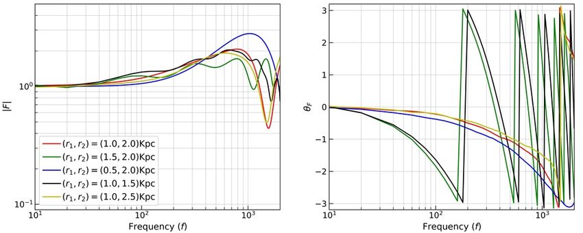
#### Page 2 of 1                                                                         J. Astrophys. Astr. (0000) 000: ####

gle plane. Erdl & Schneider (1993) presented a detailed       where κ is known as convergence and represents the di-
study of two-point mass lens in double plane lensing in       mensionless surface mass density of the lens.
the geometric optics limit and pointed out various dif-           For a lensed signal coming from the source, the cor-
ferences between single and double-plane lensing.             responding time delay (td ) with respect to the unlensed
    In the present work, we focus on the wave effects         signal is given by
in double plane lensing due to two point mass lenses.
                                                                   ξ02 Ds               (x − y)2
                                                                                      "                         #
While we consider both the point lenses as isolated
lenses for the bulk of the paper, we also briefly ex-         td =          (1 + zd )            − ψ(x) + φm (y) ,           (4)
                                                                   c Dd Dds                2
plore cases wherein these lenses are embedded in for-
eign galaxies. The method to calculate the amplifica-         where zd is the lens redshift, ξ0 is an arbitrary length
tion factor in a generalized N-plane lensing scenario is      scale used to make Equation 1 dimensionless and φm (y)
presented in Yamamoto (2003). For reference, we also          is a constant which is independent of lens properties
briefly explore the one and two-point mass single plane       and can be chosen to simplify the calculations.
lenses. To the best of our knowledge, the dependence               The above mentioned formalism of gravitational
of the amplification factor of the two-point mass single      lensing is valid as long as the Schwarzschild radius of
(or double) plane lens on its various parameters has not      the lens is much greater than the wavelength of the sig-
been studied in as much detail as what we present.            nal, i.e., RSch  λ. Hence, it is applicable in case of
    The rest of the paper is organised as follows: In         gravitational lensing of EM waves originating from a
§2., we review the basics of geometric and wave optics        distance source due to a lens in the mass range from
in gravitational lensing. In §3., we revisit the single and   stellar mass objects (∼ 1M ) to cluster of galaxies
double point mass lens in a single plane. In §4., we ex-      (∼ 1015 M ). On the other hand, if the wavelength of
plore the double plane lensing due to two point masses        the signal is of the order of the Schwarzschild radius
in detail: this is the core part of our work. Summary         of the lens, then the framework of geometric optics no
and conclusions are presented in §5..                         longer holds and we need to take wave effects into ac-
                                                              count. For light with wavelength ∼ 1µm, wave effects
                                                              are considerable if lens mass is ∼ 10−9 M .
2. Gravitational Lensing                                           For gravitational waves in the LIGO frequency
                                                              range (10 Hz-104 Hz), gravitational lensing due to
In this section, we briefly review the relevant ba-           a galaxy or a cluster of galaxies can be well de-
sics of gravitational lensing in the geometric op-            scribed using the geometric optics approach outlined
tics regime (Schneider et al., 1992) and wave optics          above. However, wave effects arise if the signal is
regime (Takahashi & Nakamura, 2003) for a single lens         lensed by stellar mass objects (10M − 104 M ; see fig-
plane. The gravitational lensing of a distant source by       ure 1 in Meena & Bagla 2020) as the corresponding
an intermediate lens mass distribution (between source        Schwarzschild radius (RSch ) is of the order of the wave-
and observer) can be described by the so-called gravi-        length of the signal (λGW ).
tational lens equation,                                            Thus, in a typical scenario of microlensing of grav-
                                                              itational waves, one cannot use geometric optics as the
y = x − α(x),                                          (1)    wave effects are not negligible: these manifest as a fre-
                                                              quency dependent amplification factor and phase shift.
where x = ξ/ξ0 , y = ηDd /ξ0 D s are the dimension-           The corresponding amplification factor which is de-
less source and image positions in the source and lens        fined as the ratio of the lensed and unlensed signals
plane, respectively, and ξ0 is an arbitrary length scale.     is given as (Nakamura & Deguchi, 1999; Takahashi &
Dd , Ds and Dds are the angular diameter distances from       Nakamura, 2003)
observer to lens, observer to source and from lens to
source, respectively. α(x) is the scaled deflection angle                   Ds ξ02 (1 + zd ) f
                                                                                                 Z
and related to the lens potential as: α(x) = ∇ψ(x). The       F ( f, y) =                            d2 x exp 2πi f td (x, y) ,

projected lens potential is given as                                           cDd Dds       i
                                                                                                                             (5)
          Z
        1
ψ(x) =       d2 x0 κ(x0 ) ln |x − x0 |,               (2)     where f is the frequency of the gravitational wave sig-
        π
                                                              nal, and the rest of the symbols have their usual mean-
with                                                          ing. One can see that the amplification factor depends
                                                              on the frequency of the GW signal. Hence, different
         Σ(x)               c2 D s                            frequency components of the signal are modulated by
κ(x) =        ,    Σcr =              ,                (3)
          Σcr              4πG Dd Dds                         varying factors, unlike the case of achromatic lensing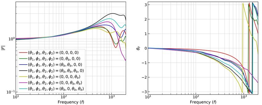
J. Astrophys. Astr. (0000)000: ####                                                                         Page 3 of 1 ####

in the regime of geometric optics. As the amplification         3.2 Single Plane Two-Point Mass lens
factor, F( f, y), is a complex quantity, wave effects mod-
                                                                In a typical galaxy, approximately half of the stellar
ify both the amplitude and the phase of the GW signal.
                                                                mass objects are in binary systems. Hence, a two-point
     As we transition towards high frequencies (geomet-
                                                                (binary) mass lens is a natural generalization of the iso-
ric optics regime), the integral in the above equation
                                                                lated point mass lens (Schneider & Weiss, 1986). The
turns highly oscillatory and only the stationary points
                                                                lensing potential corresponding to a two-point mass
of the time delay (td ) contribute significantly. The form
                                                                lens is given as
of Equation 5 in geometric optics is
            Xq                                                ψ (x1 , x2 ) = µ1 ln (x − L) + µ2 ln (x + L) ,            (8)
F ( f, y) =         |µ j | exp 2πi f td, j − iπn j ,    (6)
             i                                                  where (µ1 , µ2 ) = (M1 /MT , M2 /MT ), with MT = M1 +
                                                                M2 . For a two-point mass lens, one can always choose
where td, j is the value of time delay for j-th image, µ j is
                                                                a coordinate system in which both point masses lie
the amplification of the j-th image and n j is the Morse
                                                                on the x-axis and are at equal distance from the cen-
index with values 0, 1/2, 1 for images corresponding to
                                                                ter. Hence, the distance vectors for the first and second
minima, saddle and maxima of the time delay function,
                                                                point masses are (L, 0) and (−L, 0), respectively.
respectively. One can see that phase of the lensed GW
                                                                      A two-point mass lens system can be described by
signal corresponding to saddle (maxima) gets modified
                                                                a total of five parameters, namely, the source position
by e−iπ/2 (e−iπ ).
                                                                (y1 , y2 ), the lens masses (M1 , M2 ), and their separa-
                                                                tion 2L. Depending on the values of these parameters,
3. Single Plane Lensing                                         one obtains either a three or a five-image configura-
                                                                tion. Gravitational lensing due to a binary lens in ge-
3.1 Single Plane One-Point Mass lens                            ometric optics has already been studied in great detail
                                                                (e.g., Schneider & Weiss, 1986; Witt & Petters, 1993;
Although one cannot solve Equation 5 analytically for           Asada, 2003; Pejcha & Heyrovský, 2009; Bozza et al.,
general lens mass models, the isolated point mass lens          2020). However, the same is not true for the wave op-
model has an analytical solution (Peters, 1974):                tics regime.
                    "
                      πω iω
                                 (
                                        ω
                                                      )#              Figure 2 shows the F( f ) curves for a binary lens
   F (ω, y) = exp          +        ln      − 2φm (y)           with different values of the above mentioned parame-
                       4       2         2                      ters. The corresponding caustics and critical line plots
                       iω        iω     iω                  are shown in Figure 8 in Appendix A.. The top panel
                Γ 1−         1 F1      , 1; y2 ,         (7)
                         2           2      2                   in Figure 2 shows the amplitude (|F|) and phase shift
where ω = 8πG(1 + zd )ML f /c                                   (θF ) in the left and right panel, respectively, for different
                                    , yp= |y|, φm (y) =
                                    3
                                                                source positions keeping the lens masses and the sepa-
(xm − y) /2 − ln xm with xm = y + y2 + 4 /2. Here
         2
                                                                ration vector fixed. Here, we fix lens masses (M1 , M2 )
we have used the Einstein radius of the lens system as          and the separation vector (L) to be (50M , 50M ) and
                                                     1/2
the relevant scale length: ξ0 = 4GML Dd Dds /c2 Ds .            (0.5, 0), respectively. Analogous to a single point mass
     The amplification factor of an isolated point mass         lens, as we move towards the center, the amplitude of
lens depends on two parameters: the lens mass ML ,              the fluctuations in amplitude and phase shift increases
and the source position (y) in the source plane. Figure 1       and the frequency of the oscillations decreases. How-
shows the dependency of F( f ) on these two parameters.         ever, the presence of extra images due to the binary
The top row represents the absolute value of the ampli-         lens introduces further fluctuations in the amplitude and
fication factor (|F|) and the phase shift (θF ) in left and     phase shift. Instead of the source position, if we vary
right panel, respectively, for different source positions       the mass of the two components of the binary (centre
(y). Here the lens mass (ML ) has been fixed at 100M .          panel), at low frequency ( f < 100Hz), we make ob-
Similarly, the bottom row represents the variation in           servations similar to the previous case (and the isolated
the lens mass ML with a fixed source position y = 1.            point mass lens). However, at f > 100Hz, we notice
One can see that for a fixed lens mass, variations in the       differences due to the varying number of images, the
source position changes the amplitude of the oscilla-           time delay between these images, and the magnifica-
tions. As we move the source towards the center, the            tion of the various images. This can be seen in the
amplitude of the oscillations increases. However, the           green and blue curves which correspond to (M1 , M2 )
frequency of the oscillations decreases. On the other           = (50M , 50M ) and (70M , 30M ). Both these con-
hand, the amplitude of the oscillations is fixed if we          figurations give rise to a five-image geometry (centre
fix the source position, and only the rate of oscillations      panel of Figure 8). However, the blue curve shows sig-
change as we vary the lens mass.                                nificant de-amplification compared to the one in green.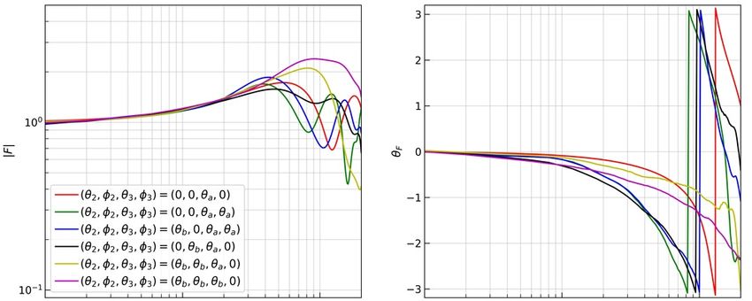
#### Page 4 of 1                                                                             J. Astrophys. Astr. (0000) 000: ####

Figure 1. Gravitational lensing due to point mass lens: The top row represents the amplification factor (|F|) and phase shift
(θF ) due to a point mass lens of 100M with different source positions (y) in left and right panel, respectively. Similarly,
the bottom row shows the amplification factor and phase shift factor due to a point lens with different lens mass values and
source position, y = 1.

In the bottom panel, we vary the separation between             is the corresponding impact parameter in the first (sec-
the two lenses by fixing the source position to (0.1, 0.1)      ond) lens plane, respectively. Due to the additional
and lens masses to (50M , 50M ). For the case of small          deflection (introduced by the second lens plane), the
values of L, we converge towards the point mass lens as         gravitational lens equation no longer remains a gradient
expected (L = 0.1; black curve). Increasing the separa-         mapping from image to source plane, leading to new in-
tion leads to different types of interference patterns de-      teresting image properties (in geometric optics approx-
pending on the number of images and the correspond-             imation). The time delay function in case of double-
ing time delays.                                                plane lensing is given as

                                                                td (x1 , x2 , y) = t12 (x1 , x2 ) + t23 (x2 , y),                 (2)
4. Double-Plane Lensing
                                                                and
The presence of a second lens plane contributes an ad-
                                                                                   1 + zi Di D j (xi − x j )2
                                                                                                "                            #
ditional deflection angle in the gravitational lens equa-       ti j (xi , x j ) =                            − βi j ψ1 (xi ) ,   (3)
tion (in thin lens approximation) given as (in dimen-                                c     Di j       2
sionless form; Schneider et al. 1992),
                                                                where βi j = Di j D s /D j Dis is a combination of various
y = x1 − α1 (x1 ) − α2 (x2 ),                            (1)    angular diameter distances related to the lens system
                                                                with the indices i, j = 1, 2, 3, i < j and j = 3 represents
where y is the unlensed source position in the source           the source plane. The rest of the symbols have their
plane. α1 (α2 ) is the scaled deflection angle and x1 (x2 )     usual meaning.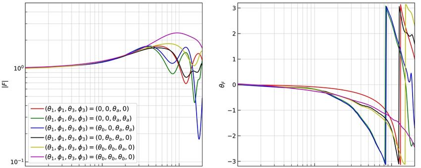
J. Astrophys. Astr. (0000)000: ####                                                                              Page 5 of 1 ####

Figure 2. Gravitational lensing due to binary lens: The top row represents the amplification factor (|F|) and phase shift
(θF ) due to a binary lens with binary lens masses of (M1 , M2 ) = (50M , 50M ) at a separation (L) = 0.5. The different
values of (y1 , y2 ) are mentioned in the left panel. The middle row represents the variation in lens masses while fixing
the source position to (y1 , y2 ) = (0.1, 0.1) and at a separation of (L) = 0.5. The bottom row represents the variation in
the separation vector while fixing the source position to (y1 , y2 ) = (0.1, 0.1) and binary lens masses (M1 , M2 ) = (50M , 50M ).

    Similar to §3., the above mentioned equations are              has been presented in Yamamoto (2003) using path in-
valid only within the regime of geometric optics. To               tegral formalism developed in Nakamura & Deguchi
study the wave effects in double plane lensing, one                (1999). In the case of N-plane lens system, the am-
needs to generalize Equation 5. Such a generalization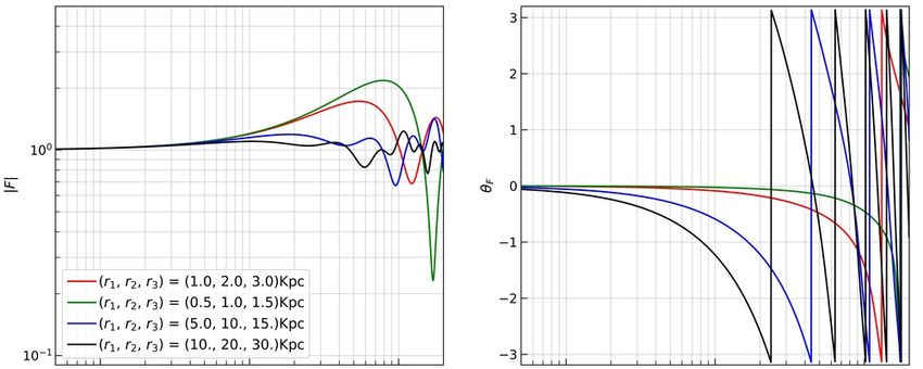
#### Page 6 of 1 J. Astrophys. Astr. (0000) 000: ####
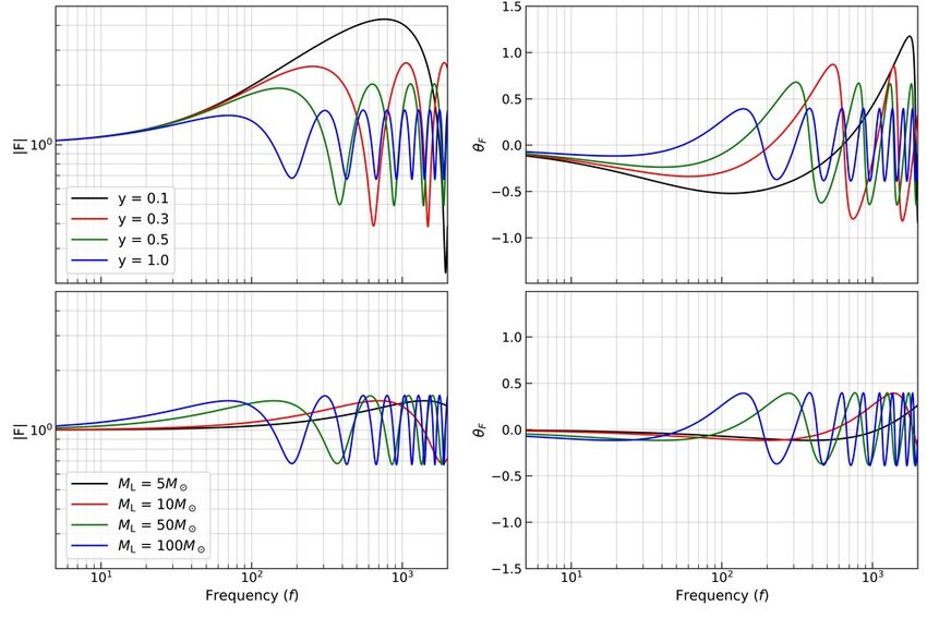
Figure 3. Dependence of the amplification factor (absolute value on the left, and phase (∆Φ = −i ln[F/|F|]) on the right)
on various parameters for the special case (Equation 6). We vary one parameter at a time, while keeping the others fixed
(with values as explained in detail in the main text). Top panel: As M1 increases, oscillations become more rapid, and the
maximum value of amplification increases as well. Centre panel: Similar to the previous case, oscillations become more
rapid, but there is no rise in value of amplification. Also, oscillations here are more rapid in comparison to the previous case.
Bottom panel: Angular position of the observer is varied. When the observer is closer to the line joining the source with the
two lenses, oscillations are slower, but the amplification is larger. As θ3 reduces, we also note that the curves tend to converge.
plification factor is given by (Yamamoto, 2003): (4)
Z where different xi represent two dimensional vectors
F ( f, y) = C f N
d x1 ...d xN exp 2πi f td (x1 , ..., xN , y)
2 2 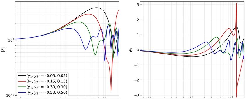
J. Astrophys. Astr. (0000)000: ####                                                                               Page 7 of 1 ####

Figure 4. Dependence of the amplification factor on the radial distances of the three objects for the special case (Equation 6).
While there are multiple ways to vary the three distances, we do so by maintaining a constant ratio between the three values.
In the top panel, we fix the angular position of the observer, while we fix the transverse distance of the observer in the bottom
panel. In the former case, we note that greater values of (r1 , r2 , r3 ) lead to an increase in rate of oscillation, coupled with a
drop in the maximum value of amplification. Trends are opposite in the bottom panel.

in different lens planes. f represents the frequency                   §4.3. Performing this ‘2N’ integral (Equation 4) using
of the signal. The time delay function is given by                     standard quadrature methods is not a very efficient pro-
td (x1 , ..., xN , y) = Σi=1
                         N
                             ti,i+1 (xi , xi+1 ) with xN+1 = y. C is   cess. Hence, for these general cases, we use a Monte
a factor which depends on the various angular diameter                 Carlo integrator provided by the vegas package (Lep-
distances under consideration and given as                             age, 2020).

      −i N YN                                                        4.1 The Special Case
                           D0,i D0,i+1
C=               (1 + zi )             ,                        (5)
       c     i=1
                            Di,i+1                                     Consider two point mass lenses with masses M1 and
                                                                       M2 , at distances r1 and r2 (from the source) respec-
where zi is the redshift for the i-th lens plane and                   tively, that are co-linear with the source. For an ob-
D0,i , D0,i+1 , and Di,i+1 are the angular diameter dis-               server at a distance r3 and angular position θ3 , the am-
tances between observer and i-th lens plane, observer                  plification factor is given by (Yamamoto, 2003):
and (i+1)-th lens plane, and i-th and (i+1)-th lens plane.
     In general, Equation 4 needs to be solved numer-
ically. However, for a special case of double-plane
lensing (N = 2), one can obtain an analytic expression
(Yamamoto, 2003). This special case is discussed in
§4.1. More general cases are discussed in §4.2 and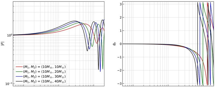
#### Page 8 of 1                                                                              J. Astrophys. Astr. (0000) 000: ####

                                                                       M . As θ3 decreases, i.e. as the observer approaches
                                                                       the line joining the source with the two lenses, two
                                           πkGMT
                                                    !
     F(k, θ3 ) = exp(iα) exp                     Γ (1 − χ1 )           qualitative trends take place: oscillations become less
                                             c2                        rapid, and the maximum value of (modulus of) the am-
                           ∞
                           X (−i)L                                     plification factor increases. This is qualitatively similar
                       z                 Γ (1 + L − χ2 ) (xz)L         to what one observes in the single lens plane case. We
                                 (L!)2
                           L=0                                         also note that the behaviour of the amplification factor
                       2 F1   (1 − χ1 , 1 + L − χ2 , 1 ; 1 − z) (6)    tends to converge as θ3 reduces (e.g. the cyan and pink
                                                                       curves almost superimpose on one another).
where                                                                        In Figure 4, we vary (r1 , r2 , r3 ) while fixing M1 =
                                                                       10 M , M2 = 10 M . In the top panel, we fix the angu-
MT B M1 + M2 ,             k B (2π f )/c,                        (7)   lar position of the source (θ3 = 0.009 arcsec). While the
                                                                       three distances can be varied in multiple ways, we do so
                                                                       by fixing the ratio between the three values. As the dis-
        2ikGM1                   2ikGM2                                tances get larger, oscillations are more rapid, and the
χ1 B           ,       χ2 B             ,                        (8)
           c2                       c2                                 maximum value of amplification is smaller. We note
                                                                       the similarity in observations with those of the bottom
                                                                       panel of Figure 3: increasing θ3 while keeping the three
     r3 (r2 − r1 )                kr2 r3 θ32                           distances fixed is analogous to keeping θ3 fixed while
zB                 ,   xB                    ,                   (9)
     r2 (r3 − r1 )               2(r3 − r2 )                           increasing the three distances – both lead to an increase
                                                                       in the length of the perpendicular dropped from the ob-
α is a real constant corresponding to a constant phase                 server to the line joining the source with the two lenses.
difference, and 2 F1 (a, b, c; d) is the Hyper-geometric                     Instead of fixing the value of θ3 while varying
function.                                                              (r1 , r2 , r3 ), one can alternatively fix the value of the
      For the special case under consideration, there are              above mentioned perpendicular distance. We show
six different parameters on which the amplification fac-               these trends in the bottom panel of Figure 4 where we
tor depends, namely, r1 , r2 , r3 , θ3 , M1 and M2 . In Fig-           fix the perpendicular distance to be ∼4×10¹² meters.
ure 3, we vary these parameters one at a time. For each                Once again, we note similarities to the bottom panel of
case, the absolute value of the amplification factor is                Figure 3: as the magnitude of (r1 , r2 , r3 ) increases, the
shown on the left, while the phase is shown on the right.              angular position of the observer is effectively reduced,
In the top panel, we fix (r1 , r2 , r3 ) = (1.0, 2.0, 3.0) kpc,        and we observe that the oscillations of the amplification
M2 = 10 M , θ3 = 0.009 arc-sec, and vary M1 . As M1                    factor become less rapid, and the maximum value of
increases, oscillations become more rapid, and this is                 (modulus of) the amplification factor increases. Also,
accompanied by an increase in the maximum value of                     the curves tend to converge for large values of the three
the amplification factor. In the centre panel, we vary                 distances.
the value of M2 , while keeping M1 = 10 M and other
parameters fixed at the values mentioned above. As M2                  4.2 Relaxing the Co-linearity Condition
increases, we again notice that the oscillations become
rapid, and the maximum value of the amplification fac-                 In this sub-section, we relax the condition that requires
tor also does increase slightly. However, in the case of               the two lenses to be co-linear with the source. Once
varying M2 , oscillations are more rapid than in the case              we relax the same, there are two possible scenarios that
of varying M1 , and the maximum value of amplification                 one can consider: (1) In-Plane variation of angular po-
does not change as sharply as in the case of varying M1 .              sitions: the source, lenses and the observer lie along
For instance, the black curve in the centre left panel os-             the same plane. This introduces two additional param-
cillates with a frequency of ∼ 500 Hz, while the fre-                  eters in the analysis, namely, θ1 and θ2 – the angular
quency of oscillation of the black curve in the top left               positions of the two lenses with respect to the source.
panel is ∼ 700 Hz. This set of observations suggest                    (2) Off-Plane variation of angular positions: the source,
the following: the mass of the lens closer to the source               lenses and the observer no longer lie along the same
(M1 ) has a greater affect on the maximum value of the                 plane. In addition to θ1 and θ2 , this case has three more
modulus of amplification, while M2 is more important                   parameters, namely, φ1 , φ2 , φ3 – the angles (measured
with respect to the rate at which the amplification factor             from the source) subtended by the off-plane object with
oscillates. We also note the difference in behaviour of                respect to the plane of the paper.
the phase at large M1 .                                                     We start with the In-Plane case, where the two
      In the bottom panel, we vary θ3 while fixing                     lenses, the source and the observer all lie along the
(r1 , r2 , r3 ) = (1.0, 2.0, 3.0) kpc, and (M1 , M2 ) = (10, 10)       same plane. The corresponding absolute values and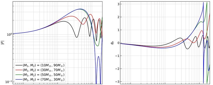
J. Astrophys. Astr. (0000)000: ####                                                                             Page 9 of 1 ####

Figure 5. In-Plane Variation of angular positions – Top Panel: Varying the angular position of the two lenses. As elaborated
in the main text, the lens closer to the source (M1 ) seems to have a greater effect on the range of |F| values, while the rate of
oscillation of the |F| curve seems to have a greater dependence on M2 . Bottom Panel: Varying the radial distance of lenses
at fixed values of other parameters. The dependence of the amplification factor on these two parameters seems to be more
complex than the dependence on angular positions.

phase of the amplification factors are shown in Figure            position of M2 seems to have a greater affect on the rate
5. In the top panel, we choose (r1 , r2 , r3 ) = (1.0, 2.0,       of oscillation in comparison to the maximum value of
3.0) kpc, (M1 , M2 ) = (10, 10) M , θ3 = 0.009 arc-sec,           amplification. Comparing the blue and green curves,
and vary the values of (θ1 , θ2 ). In red, for reference, we      we note the opposite for the angular position of M1 ,
consider (θ1 , θ2 ) = (0, 0), which is the same as some           which seems to have a greater effect on the maximum
of the curves from Figure 3. For the green and blue               value reached by the amplification factor as it oscillates.
curves, we choose (θ1 , θ2 ) = ( 2θ33 , −2θ
                                         3 ) and ( 3 , 3 ).
                                            3     −2θ3 −2θ3
                                                                       In the bottom panel of Figure 5, we continue to
These two curves oscillate faster than the curve in red,          choose (M1 , M2 ) = (10, 10) M and θ3 = 0.009 arc-sec.
with the blue curve portraying faster oscillations than           In addition, we fix (θ1 , θ2 ) = ( −2θ
                                                                                                       3 , 3 ). For reference,
                                                                                                         3 2θ3

the curve in green: oscillations are most rapid when              in red, we show the case with (r1 , r2 ) = (1.0, 2.0) kpc.
both the lenses are away from the line joining the source         With the green and blue (black and yellow) curves, we
with the observer. In the curve in black, we place M2             vary r1 (r2 ) with r2 (r1 ) fixed at 2.0 (1.0) kpc. With the
closer to the line joining the source with the observer,          first two set of curves, we see that the rate of oscilla-
with (θ1 , θ2 ) = ( −2θ
                     3 , 3 ). In this case, the curve oscil-
                        3 2θ3                                     tion of the amplification factor increases (reduces) as
lates slower in comparison to the red curve. While the            M1 moves away (closer) to the source. However, with
angular positions of both lenses have an impact on both           M2 , we note the opposite: oscillations are more (less)
the rate of oscillation and the maximum value of ampli-           rapid when r2 is smaller (larger). Unlike in Figure 5, we
fication, we note the following difference: the angular           see that the (radial) position of both the lenses can have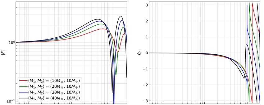
#### Page 10 of 1                                                                           J. Astrophys. Astr. (0000) 000: ####

Figure 6. Off-Plane Variation of angular positions – For simplicity, angles are represented by this set of variables: (θa , θb ) =
(0.009 arc-sec, (2/3)θa )rad. As elaborated in the main text, in each panel, we choose one object (along with the source) to
form the primary axis of the plane under consideration. One of the other two objects are displaced off-plane. We note that
trends are not always similar to in-plane variation of angular positions.

a significant impact on the rate of oscillation. How-             value of amplification. We thus already begin to see
ever, only the (radial) position of M1 greatly effects the        the complex dependence of the amplification factor on
maximum value of amplification. This is as opposed to             the various parameters, wherein trends are not easy to
the top panel of Figure 5, where the (angular) position           extrapolate.
of both the lenses do have an effect on the maximum                   Finally, in Figure 6, we show the Off-Plane case.
J. Astrophys. Astr. (0000)000: ####                                                                        Page 11 of 1 ####

Figure 7. Variation of convergence and shear parameters for the case described in §4.3. In the top (centre) panel, we examine
cases with only external shear (convergence). In the bottom panel, we consider non-zero values of both external shear and
convergence. External shear seems to have a greater effect on the rate of oscillation, while external convergence modifies the
amplification, more so at low frequencies.

As mentioned above, this introduces three additional            axis of the plane to be the line joining the source with
parameters: φ1 , φ2 , φ3 , along with the In-Plane parame-      a given object (lens/observer). The second axis is con-
ters, θ1 , θ2 . Although there are numerous ways in which       sidered to be the perpendicular dropped from one of the
these parameters can be varied, we choose the follow-           other two objects onto the primary axis. These two axes
ing scheme: in each panel, we consider the primary              form the plane, and the third (remaining) object is dis-
#### Page 12 of 1                                                                            J. Astrophys. Astr. (0000) 000: ####

placed out of this plane. In all plots, we fix (r1 , r2 , r3 )   source with the observer as the primary axis. Curves
= (1.0, 2.0, 3.0) kpc, (M1 , M2 ) = (10, 10) M . For             two - four (five - seven) consider off-plane displace-
simplicity, we define θa = 0.009 arc-sec and θb = 2θ3a .         ments of M1 (M2 ). The curve in green considers an
Whenever not varied, we fix (θ1 , φ1 ) = (θ2 , φ2 ) = (0, 0),    off-plane displacement of M1 away from the observer.
and (θ3 , φ3 ) = (θa , 0) rad.                                   From Figure 5, one would expect the curve in green to
     In the top panel, we consider the line joining the          oscillate faster than the one in red, but such a trend is
source with M1 as the primary axis. For reference, in            not seen. However, we note that a slight reduction in
red, we show the case for which the two lenses are co-           the maximum value of amplification, as expected. The
linear with the source. The green and blue curves con-           curve in blue considers a displacement of M1 towards
sider the displacement of the observer from the plane.           the observer, and as expected, this is accompanied by
Both these curves oscillate faster than the reference,           an increase in the maximum value of amplification. The
with the curve in green oscillating faster than the one          curve in black considers an in-plane displacement of
in blue. However, the difference in rates of oscillation         M2 towards the source, and as expected from previ-
is not as large as one would expect from a compari-              ous plots, the rate of oscillation drops. However, we
son with Figure 5. The remaining three curves con-               also note a very sharp increase in the maximum value
sider the displacement of M2 out of the selected plane.          of amplification, which hasn’t always been observed in
With respect to the reference, the curve in black con-           earlier plots. The curves in yellow and pink consider
siders a displacement of M2 away from the observer.              displacements of M2 away and towards the observer,
As expected from previous Figures, oscillations grow             respectively. As expected, we note an increase and
more rapid, and the modulus curve oscillates to com-             decrease in the rate of oscillation, respectively. With
paratively smaller values. The curve in yellow con-              the curve in cyan, we consider a displacement of M1
siders a displacement towards M2 (albeit an ‘in-plane’           towards the observer, and in agreement with previous
displacement). In this case, we notice that oscillations         plots, we note an increase in the maximum value of am-
grow slower and the modulus values oscillate to larger           plification.
values, both of which are in agreement with earlier ob-
servations. In the curve in pink, we reduce the angle            4.3 Effect of External Perturbations
of the observer, which essentially brings the observer
                                                                 So far, we have explored cases where both point mass
closer to M2 . The observed trend is what one would
                                                                 lenses have been treated as isolated objects in their re-
expect from Figure 5: oscillations begin to slow down,
                                                                 spective lens planes. While this is a starting point for
and modulus values begin to increase.
                                                                 lens systems within our own galaxy, a further general-
     In the centre panel, we consider the line joining the
                                                                 ization is required when lenses are embedded in host
source with M2 as the primary axis. Akin to the pre-
                                                                 galaxies. In this subsection, we consider an extension
vious case, the green and blue curves consider the dis-
                                                                 of the special case discussed in §4.1: scenarios wherein
placement of the observer from the plane. Observations
                                                                 the two micro-lenses are collinear with the source, and
are qualitatively similar to the previous case: the green
                                                                 the two micro-lenses are embedded in two distinct host
and blue curves oscillate faster than the reference, with
                                                                 galaxies. We assume that the effect of the host galaxy
the green curve oscillating slightly faster. Once again,
                                                                 is constant across the Einstein radius of the microlens.
the difference in rates of oscillation is smaller than ex-
                                                                 Under this framework, the following terms are intro-
pected. In the remaining three curves, M1 is displaced
                                                                 duced into the lensing potential (an extension of the
off-plane. The black curve considers displacement of
                                                                 single-plane case discussed in Schneider et al. (1992)):
M1 away from the observer. As opposed to previous ob-
servations, absolute values are similar to the reference,
and the rates of oscillation are also comparable. How-
                                                                                                             ψext (x1 , x2 , x3 , x4 ) =
ever, if we consider an additional in-plane displacement                         !h
(yellow curve), the modulus values begin to rise, but not              r1 r3                                                           i
                                                                                      κ1 (x12 + x22 ) + γ11 (x12 − x22 ) + 2γ12 x1 x2
as large as one would expect from Figure 5. Reducing                2(r3 − r1 )
θ3 (pink curve) seems to increase the modulus values,                 r2 r3
                                                                               !h                                                i
which is as expected, but the rate of oscillation drops          +                κ2 (x32 + x42 ) + γ21 (x32 − x42 ) + 2γ22 x3 x4 ,
                                                                   2(r3 − r2 )
significantly, which contradicts Figure 5. We thus see
that a combination of In-Plane and Off-Plane displace-                                                                         (10)
ments lead to trends that are not always in agreement
with In-Plane displacements alone, and the difference                where κ1 (κ2 ) and (γ11 (γ21 ), γ12 (γ22 )) correspond to
is larger for M1 .                                               the external convergence and shear parameters of the
     In the bottom panel, we consider the line joining the       galaxy in which M1 (M2 ) is embedded. For simplicity,
                                                                 we choose γ12 and γ22 to be zero, which correspond to
J. Astrophys. Astr. (0000)000: #### Page 13 of 1 ####
specific orientations of the two galaxies. Note that the wave-optical effects of a double plane lens with a single
various xi ’s in Equation 10 correspond to angular co- lens plane consisting of one and two-point mass lenses.
ordinates. We find that only for some arrangements one can iden-
We show the dependence of the amplification fac- tify similar behavior in single and double plane lens-
tor on the various external convergence/shear parame- ing. For example, in some cases, varying the observer
ters in Figure 7. For reference, in each of the panels, position with respect to the source yields a qualita-
we show the isolated microlenses case in black. To en- tively similar behavior in both single and double planes.
sure that numbers are meaningful with respect to galaxy However, apart from this, it is not straightforward to
lenses, we choose (r1 , r2 , r3 ) = (100.0, 200.0, 300.0) make generalized statements about the behavior of lens
Mpc. We fix θ3 = 0.00003 arc-sec and microlens systems: the number of parameters is just too large,
masses are set to 10 M each. For this choice of θ3 , even for the relatively simple case of two lens planes.
the curve in black is identical to the red curves from the One would expect the complexity to further in-
previous figures. crease for a large number of lens planes. However,
In the top panel, we consider cases with only exter- the probability of observing lens system with more than
nal shear (i.e. κ’s are set to zero). When one/both of the two lens planes is significantly lower. The increase in
two shear parameters is/are non-zero, we note the fol- complexity also holds for double plane lenses if we in-
lowing: absolute value and phase of the amplification crease the number of point mass lenses in one or both of
factor oscillate at different rates in comparison to the the lens planes. The presence of galaxy lenses in such
reference curve in black. In the centre panel, we con- systems would introduce an additional shear and con-
sider cases with only external convergence. Unlike the vergence, which is expected to further complicate the
previous case with only external shear, we notice a pat- analysis. Keeping this in mind, we conclude that the
tern in this case: ‘adding’ external convergence into the best way to study wave effects in multi-plane lensing is
lens system increases the magnitude of absolute values to tackle separate lens systems case by case instead of
of the amplification factor at low frequencies (∼10Hz). hoping to make predictions based on a few test cases.
In the bottom panel, we examine cases where both ex-
ternal convergence and shear are present in the lens sys-
tem. One can see that the resultant curves with both Acknowledgements
non-zero shear and convergence look like combinations
of the above panels: the non-zero convergence leads to RR would like to thank the Department of Science and
an increase in the overall magnitude of the oscillations, Technology, Government of India for being awarded
while the non-zero shear introduces a modification in the INSPIRE scholarship. AKM would like to thank
rate of oscillation. Council of Scientific and Industrial Research (CSIR)
As mentioned earlier, these observations depict the India for financial support through research fellowship
complex dependence of the amplification factor on the No. 524007. Authors acknowledge the use of IISER
various parameters. Unlike the single lens plane case Mohali HPC facility. Authors would like to thank Kan-
(especially for the isolated point mass lens), it isn’t easy daswamy Subramanian for valuable comments on the
to make predictions on the behaviour of the amplifi- manuscript. This research has made use of NASA’s As-
cation factor when the values of multiple parameters trophysics Data System Bibliographic Services.
are varied simultaneously. From our observations, we
recommend that the best way to study wave effects in
double- (or multi-, in general) plane lensing is to study References
various possible lens systems case by case, instead of
trying to extrapolate results from a set of test cases. Abbott, B. P., Abbott, R., Abbott, T. D., et al. 2019,
Apart from that, we also find that the Monte Carlo inte- Physical Review X, 9, 031040
grator provides satisfactory results for the case of N =
2. However, for integrals corresponding to higher num- Abbott, R., Abbott, T. D., Abraham, S., et al. 2020,
ber of lens planes, one may need to explore alternate arXiv e-prints, arXiv:2010.14527
methods (e.g., Feldbrugge, 2020). Asada, H. 2003, Progress of Theoretical Physics, 110,
425
5. Conclusions Baraldo, C., Hosoya, A., & Nakamura, T. T. 1999,
Phys. Rev. D, 59, 083001
In this work, we have explored the effects of wave op-
tics in double plane lensing. We have also compared the Bartelmann, M. 2010, Classical and Quantum Gravity,
27, 233001#### Page 14 of 1 J. Astrophys. Astr. (0000) 000: ####
Bozza, V., Pietroni, S., & Melchiorre, C. 2020, Uni- Umetsu, K. 2020, A&A Rev., 28, 7
verse, 6, 106
Witt, H. J., & Petters, A. O. 1993, Journal of Mathe-
Broadhurst, T., Diego, J. M., & Smoot, G. F. 2020, matical Physics, 34, 4093
arXiv e-prints, arXiv:2006.13219
Yamamoto, K. 2003, arXiv e-prints, astro
Broadhurst, T., Diego, J. M., & Smoot, George, I. 2018,
arXiv e-prints, arXiv:1802.05273
Broadhurst, T., Diego, J. M., & Smoot, George F., I. Appendix A. Geometric Optics
2019, arXiv e-prints, arXiv:1901.03190
For greater insights into Figure 2, we here show the
Christian, P., Vitale, S., & Loeb, A. 2018, Phys. Rev. D,
critical lines and caustics corresponding to the vari-
98, 103022
ous cases discussed earlier. When the source happens
Diego, J. M., Hannuksela, O. A., Kelly, P. L., et al. to be outside the caustic, three images of the source
2019, A&A, 627, A130 are formed. However, when the source moves into the
caustic, an additional two images are produced, thereby
Erdl, H., & Schneider, P. 1993, A&A, 268, 453 increasing the complexity of the amplification factor.
Feldbrugge, J. 2020, arXiv e-prints, arXiv:2010.03089
Kneib, J.-P., & Natarajan, P. 2011, A&A Rev., 19, 47
Kochanek, C. S., & Apostolakis, J. 1988, MNRAS,
235, 1073
Lepage, G. P. 2020, arXiv e-prints, arXiv:2009.05112
Li, S.-S., Mao, S., Zhao, Y., & Lu, Y. 2018, MNRAS,
476, 2220
Meena, A. K., & Bagla, J. S. 2020, MNRAS, 492, 1127
Mishra, A., Meena, A. K., More, A., Bose, S., & Singh
Bagla, J. 2021, arXiv e-prints, arXiv:2102.03946
Nakamura, T. T., & Deguchi, S. 1999, Progress of The-
oretical Physics Supplement, 133, 137
Ohanian, H. C. 1974, International Journal of Theoret-
ical Physics, 9, 425
Pejcha, O., & Heyrovský, D. 2009, ApJ, 690, 1772
Peters, P. C. 1974, Phys. Rev. D, 9, 2207
Schneider, P., Ehlers, J., & Falco, E. E. 1992, Gravita-
tional Lenses, doi:10.1007/978-3-662-03758-4
Schneider, P., & Weiss, A. 1986, A&A, 164, 237
Smith, G. P., Berry, C., Bianconi, M., et al. 2018, IAU
Symposium, 338, 98
Subramanian, K., & Chitre, S. M. 1984, ApJ, 276, 440
Subramanian, K., Rees, M. J., & Chitre, S. M. 1987,
MNRAS, 224, 283
Takahashi, R., & Nakamura, T. 2003, ApJ, 595, 1039J. Astrophys. Astr. (0000)000: #### Page 15 of 1 #### Figure 8. Caustics (left) and Critical lines (right) corresponding to the cases discussed in Figure 2. The various filled circles correspond to the position of the source (images) in the left (right) panel. When the source happens to be outside (inside) the caustic, three (five) images are formed.
You can also read