YOUTUBE SCALE, LARGE VOCABULARY VIDEO ANNOTATION
←
→
Page content transcription
If your browser does not render page correctly, please read the page content below
YouTube Scale, Large Vocabulary
Video Annotation

Nicholas Morsillo, Gideon Mann and Christopher Pal

Abstract As video content on the web continues to expand, it is increasingly im-
portant to properly annotate videos for effective search and mining. While the idea
of annotating static imagery with keywords is relatively well known, the idea of an-
notating videos with natural language keywords to enhance search is an important
emerging problem with great potential to improve the quality of video search. How-
ever, leveraging web-scale video datasets for automated annotation also presents
new challenges and requires methods specialized for scalability and efficiency.
In this chapter we review specific, state of the art techniques for video analysis,
feature extraction and classification suitable for extremely large scale automated
video annotation. We also review key algorithms and data structures that make truly
large scale video search possible. Drawing from these observations and insights, we
present a complete method for automatically augmenting keyword annotations to
videos using previous annotations for a large collection of videos. Our approach is
designed explicitly to scale to YouTube sized datasets and we present some exper-
iments and analysis for keyword augmentation quality using a corpus of over 1.2
million YouTube videos. We demonstrate how the automated annotation of web-
scale video collections is indeed feasible, and that an approach combining visual
features with existing textual annotations yields better results than unimodal mod-
els.

Nicholas Morsillo
Department of Computer Science, University of Rochester, Rochester, NY 14627, e-mail: mor-
sillo@cs.rochester.edu
Gideon Mann
Google Research, 76 Ninth Avenue, New York, NY 10011 e-mail: gideon.mann@gmail.com
Christopher Pal
Département de génie informatique et génie logiciel, École Polytechnique de Montréal, Montréal,
PQ, Canada H3T 1J4, e-mail: christopher.pal@polymtl.ca

                                                                                                   1
2 Nicholas Morsillo, Gideon Mann and Christopher Pal
1 Introduction
The web has become an indispensable resource for media consumption and social
interaction. New web applications, coupled with spreading broadband availability,
allow anyone to create and share content on the world wide web. As a result there
has been an explosion of online multimedia content, and it is increasingly important
to index all forms of content for easy search and retrieval.
Text-based search engines have provided remarkably good access to traditional
web media in the online world. However, the web is rapidly evolving into a multime-
dia format, and video is especially prominent. For example, YouTube receives over
twenty hours of new video uploads every minute. Standard search engines cannot
index the vast resources of online video unless the videos are carefully annotated by
hand. User-provided annotations are often incomplete or incorrect, rendering many
online videos invisible to search engine users.
Clearly there is an immediate need for video-based search that can delve into
the audio-visual content to automatically index videos lacking good textual annota-
tions. Video indexing and retrieval is an active research discipline that is progressing
rapidly, yet much of this research avoids the difficult issue of web-scalability. We
need robust techniques for analyzing and indexing videos, and we also need tech-
niques to scale to handle millions of clips. Furthermore, we desire that web-scale
approaches benefit from the increase in data by learning improved representations
from the expanded datasets.
In this chapter we review a portion of the image and video mining literature with
a critical eye for scalability. Our survey covers both low level visual features and
higher level semantic concepts. We observe that in contrast to the relatively new
discipline of video annotation, image annotation has received considerably more
research attention in the past. Much of the image annotation work can be transferred
to the video domain, particularly where scalability issues are involved.
Video search and mining is a broad field, and here we choose to focus on the
task of automated annotation from web datasets. We propose a novel technique to
automatically generate new text annotations for clips within a large collection of
online videos. In contrast to existing designs which may involve user feedback,
visual queries, or high level semantic categories, our approach simply attempts to
enhance the textual annotations of videos. This is beneficial as user feedback and
visual query specification can be time consuming and difficult, and our approach is
not constrained to a fixed set of categories. Additionally, the enhanced annotations
resulting from our approach can be used directly in improving existing text-based
search engines.
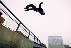
Our method is depicted in Figure 1, and an overview of the procedure is as fol-
lows. Beginning with a query video to annotate, we decompose the video into shots
using a shot boundary detector. Visually similar shots are discovered from the pool
of shots across all videos in the corpus. Then, a probabilistic graphical model is used
to decide which annotation words to transfer from neighboring shots to the query
video. Key to this approach is a scalable approximate nearest neighbor algorithm
implemented using MapReduce [9], coupled with a compact representation of shotYouTube Scale, Large Vocabulary Video Annotation 3
query video
Existing
Annotations:
parkour
compute visual similarity to corpus videos: compute co-occurrence of existing
annotation(s) with corpus annotations:
jump
people city bike jump parkour
parkour
city city -
bike 0.3 -
jump 0.2 0.9 -
bike parkour 0.6 0.1 0.8 -
sports
combine visual and textual
predictions
New Annotations: jump, city
Fig. 1 An example of our approach to generating new text annotations for online videos.
feature vectors. The probabilistic model maintains efficiency by approximating the
contributions of the majority of corpus video shots which are not found to be nearest
neighbors to a query.
Video search and mining research has traditionally involved known datasets with
fixed sets of keywords and semantic concepts, such as TRECVID [41] and the Ko-
dak benchmark dataset [26]. A key difference in our work is the absence of a con-
strained set of annotation keywords. We construct an annotation vocabulary directly
from annotations provided by users and uploaders of online videos. This permits a
larger range of annotations that are tailored for the data and it avoids costly manual
construction of vocabularies and concept ontologies. However, it also introduces
new challenges for measurement and performance evaluation, since ground truth
labels are not fixed or verified.
We conclude the chapter with preliminary results of our approach applied to a
large portion of the YouTube corpus.4 Nicholas Morsillo, Gideon Mann and Christopher Pal 2 Image and Video Analysis for Large-Scale Search Successful annotation and search is supported by deep analysis of video content. Here we review methods for analyzing and indexing visual data, and observe how these methods relate to the problem of large-scale web video search. We begin our review with image analysis techniques as many successful video analysis methods are constructed from them, and they offer unique insights into the scalability prob- lem. In some cases image techniques may be applied directly to still video frames. We then turn our attention to techniques specifically for video. 2.1 Image Analysis and Annotation Image annotation is an active field of research that serves as a precursor to video annotation in numerous ways. Video features are often inspired and sometimes di- rectly borrowed from image techniques and many methods for image indexing are also easily applied to video. Here we survey some of the most relevant static image annotation literature including modern trends in the field and adaptations of tech- niques for static image annotation to video. We also cover emerging and state of the art feature extraction techniques specifically designed for video. We review image features, indexing techniques, and scalable designs that are particularly useful for working with web-scale video collections. 2.1.1 Image Features for Annotation The relatively early work on image annotation by Mori et al. [31] used the co- occurrence of words and quantized sub-regions of an image. They divided an image into a number of equally sized rectangular parts, typically 3x3 or 7x7. They then use a 4x4x4 cubic RGB color histogram, and 8-direction and 4 resolution histogram of intensity after Sobel filtering. This procedure gives them 96 features from an im- age. Duygulu et al. [10] cast the object recognition problem as a form of machine translation and sought to find a mapping between region types and annotation key- words. They segmented images using normalized cuts then only used regions larger than a minimum threshold for their visual representation. This procedure typically lead to 5-10 regions for an image. From these regions they used k-means to ob- tain 500 blobs. They computed 33 features for each image including: region color and standard deviation, region average orientation energy (12 filters), region size, location, convexity, first moment, and the ratio of region area to boundary length squared. Their model was trained using 4500 Corel images where there are 371 words in total in the vocabulary and each image has 4-5 keywords. Jeon et al. [22] used the same Corel data, word annotations and features used in [10]. They used this vocabulary of blobs to construct probabilistic models to predict the probability
YouTube Scale, Large Vocabulary Video Annotation                                     5

of generating a word given the blobs in an image. This general approach allows one
to annotate an image or retrieve images given a word as a query.
    More recently Makadia et al. [28] have proposed a new, simple set of baseline im-
age features for image annotation problems. They also proposed a simple technique
to combine distance computations to create a nearest neighbor classifier suitable for
baseline experiments. Furthermore, they showed that this new baseline outperforms
state of the art methods on the Corel standard including extensions of Jeon et al.
[22] such as [14]. The new baseline was also applied to the IAPR TC-12 [18] col-
lection of 19,805 images of natural scenes with a dictionary of 291 words as well
as 21,844 images from the ESP collaborative image labeling game [45]. We discuss
this method in some detail because it produces state of the art results and we will
use these features in our own experimental work on video annotation. We will refer
to these features as JEC (Joint Equal Contribution) features as the authors advocate
computing distances using an equal weighting of distances computed for a given
feature type when making comparisons. JEC features consist of simple color and
texture features. Color features are created from coarse histograms in three different
color spaces: RGB, HSV and LAB. For texture, Gabor and Haar Wavelets are used.
    Color 16-bin per channel histograms are used for each colorspace. In a com-
parison of four distance measures (KL-divergence, a χ 2 statistic, L1 -distance, and
L2 -distance) on the Corel dataset, [28] found that L1 performed the best for RGB
and HSV while the KL-divergence was better suited for LAB.
    Texture Each image is filtered with Gabor wavelets at three scales and four ori-
entations. From each of twelve response images a histogram for the magnitudes is
built. The concatenation of these histograms is a refered to as feature vector ‘Gabor’.
The second component of the Gabor feature vector captures the phase by averaging
the phase over 16 × 16 blocks in each of the twelve response images. The mean
phase angles are quantized into eight values or three bits and concatenated into a
feature vector referred to as ‘GaborQ’.
    Haar wavelets are generated by block convolution with horizontally, diagonally
and vertically oriented filters. After rescaling an image to 64 × 64 pixels a ‘Haar’
feature is generated by concatenating the Haar response magnitudes. Haar responses
are quantized into the three values: 0, 1 or -1 for zero, positive and negative re-
sponses. A quantized version of the Haar descriptor called ‘HaarQ’ was also ex-
plored. They used L1 distance for all texture features.

2.1.2 Image Features for Object, Category and Scene Recognition

Object recognition, scene recognition and object category recognition can all be
thought of as special cases of the more general image annotation problem. In object
recognition there has been an lot of interest in using techniques based on SIFT de-
scriptors [27]. We briefly review SIFT here since they are representative of a general
“keypoint plus descriptor” paradigm. SIFT and other similar variants consist of two
broad steps, keypoint detection and descriptor construction. First, one detects key-
points or interest points in an image. In the SIFT approach one detects minimal or
6 Nicholas Morsillo, Gideon Mann and Christopher Pal maximal points in a difference of Gaussians scale space pyramid, but other methods use Harris corners or other interest point detection techniques. The local descriptor centered at the interest point is assigned an orientation based on the image gradient in a small region surrounding the key-point. Finally, given a scale and orientation, the SIFT descriptor itself is built from histograms of image gradient magnitudes in the region surrounding the scaled and oriented region surrounding the key-point. SIFT based techniques work well for detecting repeated instances of the same ob- ject from images of multiple views. However, other research [13] has suggested that for recognizing more variable visual concepts like natural scene categories such as forest, suburb, office, etc. it is better to build SIFT descriptors based on dense sam- pling as opposed to centered on an interest point detector. More recently histogram of oriented gradient or HoG features [7] have been receiving increased attention for more general visual recognition problems. Such features are similar to SIFT descriptors but take a dense sampling strategy. More specifically, Dalal and Triggs [7] studied each stage of descriptor computation and the effect on performance for the problem of human detection. They concluded that fine-scale gradients, fine ori- entation binning, relatively coarse spatial binning, and high-quality local contrast normalization in overlapping descriptor blocks are all important for good results. Since these observations HoG features have been a popular and effective choice for various groups participating in the Pascal Visual Object Classes challenge [11]. The Pascal challenge is a good example of a well organized competition focusing on the task of recognition and detection for a 20 object classes, namely recognizing: People, Animals - bird, cat, cow, dog, horse, sheep, Vehicles - aeroplane, bicycle, boat, bus, car, motorbike, train, and Indoor items - bottle, chair, dining table, potted plant, sofa, tv/monitor. Larger object category data sets such as CalTech101 [12] or CalTech256 [17] with 101 and 256 object categories respectively have also received considerable attention. Indeed, many of the recent developments in visual features have been motivated by improving recognition performance for these object cate- gory problems. There has been increasing interest in addressing much larger problems for ob- ject, category and scene recognition. A common theme amongst many of these ap- proaches is the use of vocabulary trees and data structures for indexing large visual vocabularies. In fact these vocabularies are typically so large that the indexing step serves to operate much like an approximate nearest neighbor computation. We dis- cuss a few prominent examples. Recently, Nistér and Stewénius [32] developed a system able to recognize in real- time specific CD covers from a database of 40,000 images of popular CDs. They also presented recognition results for 1619 different everyday objects using images of four different views of each object. For their features they use an interest point detection step obtained from Maximally Stable Extremal Regions (MSERs) [29]. They obtained an elliptical patch from the image centered at the interest point which they warped into a circular patch. From this patch they computed a SIFT descriptor. They quantized descriptors using k-means and to accelerate the matching of these features to a large database they created a hierarchical cluster tree. They used a bag
YouTube Scale, Large Vocabulary Video Annotation                                     7

of visual words representation and performed retrieval using term frequency inverse
document frequency tf-idf commonly used in text retrieval.
    In another example, Schindler et al. [37] used a similar approach for the problem
of location recognition from a city scale database of roadside images. Their imagery
continuously covered a 20 kilometer stretch of road through commercial, residen-
tial and industrial areas. Their database consisted of 30,000 images and 100 million
SIFT features. They used hierarchical k-means to obtain a vocabulary tree and they
experimented with different branching factors and techniques for identifying infor-
mative features.
    Finally, the work of Torralba et al. [42] represents an important shift towards ad-
dressing problems related to extremely large data sets. They have used text based
queries to image search engines to collect 80 million low resolution images from
the web. Natural language annotations are used such that imagery is associated with
words; however, language tags are only based on the initial query terms used to
fetch imagery and the results are noisy. However, they have been able to demon-
strate that a large database of small images is able to solve many different types
of problems. Similar to other large scale techniques they use variations of nearest
neighbor methods to leverage the information contained in large data sets.

2.2 Analyzing and Searching Videos

In contrast to static images, working with video provides a fresh set of opportuni-
ties as well as new challenges. Video carries additional modalities of information
including motion cues, trajectories, temporal structure, and audio. These additional
data streams are rife with useful, search-relevant information, but they are also very
difficult to model. While audio is an important element of video we will focus our
discussion and experiments here on visual features.

2.2.1 Adapting Methods for Static Imagery to Video

One way to obtain features for video annotation is to directly adapt techniques de-
veloped for static image annotation. For example, [14] extends and adapts the initial
static image annotation approach presented in Jeon et al. [22] to create what they
call multiple bernoulli relevance models for image and video annotation. In this ap-
proach, a substantial time savings is realized by using a fixed sized grid for feature
computations as opposed to relying on segmentations as in [22] and [10]. The fixed
number of regions also simplifies parameter estimation in their underlying model
and makes models of spatial context more straightforward. To apply their method to
video they simply apply their model for visual features within rectangular regions
to the keyframes of a video. They compute 30 feature vectors for each rectangular
region consisting of: 18 color features (including region color average, standard de-
8 Nicholas Morsillo, Gideon Mann and Christopher Pal
viation and skewness) and 12 texture features consisting of Gabor energy computed
over 3 scales and 4 orientations).
The underlying multiple bernoulli relevance model consists of a kernel density
estimate for the features in each region conditioned on the identity of the video and a
multivariate bernoulli distribution over words, also conditioned on the identity of the
video. As we shall see shortly, when we seek to use a kernel density type of approach
for extremely large datasets such as those produced by large video collections, we
must use some intelligent data structures and potentially some approximations to
keep computations tractable. The authors of [14] also argue that their underlying
bernoulli model for annotations is more appropriate for image keyword annotations
where words are not repeated compared to the multinomial assumptions used in
their earlier work [22]. The experimental analysis of the multiple bernoulli model
of [14] used a subset of the NIST Video Trec dataset [34]. Their dataset consisted of
12 MPEG files, each 30 minutes long from CNN or ABC including advertisements.
There were 137 keywords in the annotation vocabulary and they found their model
produced a mean average precision of .29 for one word queries.
The “Video Google” work of Sivic and Zisserman [40] is representative of a dif-
ferent approach to video retrieval based more on object recognition and SIFT tech-
niques. The approach allows for searches and localizations of all the occurrences of
a user outlined object in a video. Sivic and Zisserman compute two different types of
regions for video feature descriptors. The first, referred to as a Shape Adapted (SA)
region, is constructed by elliptical shape adaptation around an interest point. The
ellipse center, scale and shape are determined iteratively. The scale is determined
from the local extremum across scale of a Laplacian and the shape is determined by
maximizing the intensity gradient isotropy over the region. The second type of re-
gion, referred to as a Maximally Stable (MS) region, is determined from an intensity
watershed image segmentation. Regions are identified for which the area is station-
ary as the intensity threshold is varied. SA regions tend to be centered on corner like
features and MS regions correspond to blobs of high contrast with respect to sur-
roundings. Both regions are represented as ellipses and for a 720 × 576 pixel video
frame one typically has 1600 such regions. Each type of region is then represented
as a 128 dimensional SIFT descriptor. Regions are tracked through frames and a
mean vector descriptor is computed for each of the regions. Unstable regions are re-
jected giving about 1000 regions per frame. A shot selection method is used to cover
about 10,000 frames or 10% of the frames in a typical feature length movie resulting
in a data set of 200,000 descriptors per movie. A visual vocabulary is then built by
K-means based clustering. Using scenes represented in this visual vocabulary they
use the standard term frequency-inverse document frequency or tf-idf weighting and
the standard normalized scalar product for computation for retrieval. This approach
produced impressive query by region demonstrations and results and while it was
not directly designed for the problem of video annotation, the approach could easily
be adapted by transferring labels from matching videos.YouTube Scale, Large Vocabulary Video Annotation 9
2.2.2 More Video Specific Methods
We now turn our attention to techniques much more specifically designed for video.
Certainly it is the spatio-temporal aspect of video that gives video feature computa-
tions their distinctive character compared to techniques designed for static imagery.
The particular task of human activity recognition frequently serves as a motivat-
ing problem. Early work on activity recognition analyzed the temporal structure
of video and built a table of motion magnitude, frequency, and position within a
segmented figure [35] or involved building a table with the presence or recency of
motion at each location in an image [4]. Of course, highly specific approaches for
activity recognition can use fairly detailed and explicit models of motions for activ-
ities to be recognized. These techniques can be very effective, but by their nature,
they cannot offer general models of the information in video in the way that less
domain-specific features can.
Recent developments in video feature extraction have continued to be strongly
influenced by activity recognition problems and have been largely based on local
spatio-temporal features. Many of these features have been inspired by the success
of SIFT like techniques and the approach of Sivic and Zisserman [40] described
previously is an early example. Similar to the SIFT approach, a common strategy
for obtaining spatio-temporal features is to first run an interest point detection step.
The interest points found by the detector are taken to be the center of a local spatial
or spatio-temporal patch, which is extracted and summarized by some descriptor.
Frequently, these features are then clustered and assigned to words in a codebook,
allowing the use of bag-of-words models from statistical natural language process-
ing for recognition and indexing tasks. Considerable recent work in activity recog-
nition has focused on these types of bag-of-spatio-temporal-features approaches, of-
ten explicitly cast as generalizations of SIFT features. These techniques have been
shown to be effective on small, low resolution (160x120 pixels per frame) estab-
lished datasets such as the KTH database [38] with simple activities such as people
running or performing jumping jacks. Recent extensions of the space-time cuboid
approach [23] have been applied to learn more complex and realistic human actions
from movies using their associate scripts. This work has sought to identify complex
actions like answering a phone, getting out of a car or kissing. This work also em-
phasizes the importance of dealing with noisy or irrelevant information in the text
annotation or associated movie script.
Features based on space-time cuboids have certain limits on the amount of space
and time that they can describe. Human performance suggests that more global spa-
tial and temporal information could be necessary and sufficient for activity recogni-
tion. In some of our own recent research [30] we have proposed and evaluated a new
feature and some new models for recognizing complex human activities in higher
resolution video based on the long-term dynamics of tracked key-points. This ap-
proach is inspired by studies of human performance recognizing complex activities
from clouds of moving points alone.10 Nicholas Morsillo, Gideon Mann and Christopher Pal
2.3 TRECVID
TRECVID [41] is an ongoing yearly competitive evaluation of methods for video
indexing. TRECVID is an important evaluation for the field of video search as it
coordinates a rigorous competitive evaluation and allows the community to gauge
progress. For these reasons we briefly review some relevant elements of TRECVID
here and discuss some recent observations and developments. More details about
the 2008 competition are given in [34].
One of the TRECVID tasks is to identify “high level features” in video. These
features can be thought of as semantic concepts or annotation words in terms of
our ongoing discussion. The following concepts were used for the 2008 evalua-
tion: classroom, bridge, emergency vehicle, dog, kitchen, airplane flying, two peo-
ple, bus, driver, cityscape, harbor, telephone, street, demonstration or protest, hand,
mountain, nighttime, boat or ship, flower, singing. Given the visual concepts and a
common shot boundary reference, for each visual concept evaluators return a list of
at most 2000 shots from the test collection, ranked according to the highest possibil-
ity of detecting the presence of the visual concept (or feature in the TRECVID lan-
guage). In 2004, Hauptmann and Christel [19] reviewed successful past approaches
to the challenge. Their conclusions were that combined text analysis and computer
vision methods work better than either alone; however, computer vision techniques
alone perform badly, and feature matching only works for near-duplicates. It is inter-
esting to note that this supports the notion that with a much larger corpus there is a
much better chance of finding near duplicates. In contrast to TRECVID, in our own
experiments that we present at the end of this chapter we are interested in dramati-
cally scaling up the amount of data used to millions of videos as well as extending
the annotation vocabulary to a size closer to the complete and unrestricted vocab-
ulary of words used on the web. The evaluation for this type of scenario poses the
additional real-world challenge of working with noisy web labels.
2.4 The Web, Collaborative Annotation and YouTube
The web has opened up new ways to collect, annotate store and retrieve video. Var-
ious attempts have been made to solve the annotation problem by allowing users on
the web to manually outline objects in imagery and associate a text annotation or
word with the region. The LabelMe project [36] represents a prominent and repre-
sentative example of such an approach. In contrast, Von Ahn et al. have developed a
number of games for interactively labeling static images [45, 46]. These methods are
attractive because the structure of the game leads to higher quality annotations and
the annotation process is fun enough to attract users. These projects have been suc-
cessful in obtaining moderate amounts of labeled data for annotation experiments;
however, the rise of YouTube has opened up new opportunities of unprecedented
scale.YouTube Scale, Large Vocabulary Video Annotation 11
YouTube is the world’s largest collection of video. In 2008 it was estimated that
there are over 45,000,000 videos in the YouTube repository and that it is growing
at a rate of about seven hours of video every minute [2]; in 2009 that rate was
measured at twenty hours of video per minute. Despite this there has been relatively
little published research on search for YouTube. Some recent research as examined
techniques for propagating preference information through a three-month snapshot
of viewing data [2]. Other works have examined the unique properties of web videos
[48] and the use of online videos as training data [44]. In contrast, we are interested
in addressing the video annotation problem using a combination of visual feature
analysis and a text model. YouTube allows an uploader to associate a substantial text
annotation with a video. In our own experimental analysis we will use the title of the
video and this annotation as the basis of the text labels for the video. While there are
also facilities for other users to comment on a video, our initial observations were
that this information was extremely noisy. We thus do not use this information in
our own modeling efforts. In the following section we will discuss some of the key
technical challenges when creating a solution to the video annotation problem for a
video corpus the size of YouTube.
3 Web-Scale Computation of Video Similarity
Any technique for automatic annotation on YouTube must be designed to handle
vast amounts of data and a very large output vocabulary. With traditional classi-
fication approaches, a new classifier must be trained for each distinct word in the
vocabulary (to decide how likely that particular word is to be an appropriate la-
bel for that video). Clearly, this approach cannot support a vocabulary size in the
hundreds of thousands. In our scenario, retrieval based approaches offer an appeal-
ing alternative, since one similarity function can be used to transfer an unbounded
vocabulary. These issues motivate the following discussion on nonparametric ap-
proaches to computing visual similarity. The methods detailed in this section are
designed for scalability and we focus on those that have been applied experimen-
tally in the literature to large scale image and video problems.
We begin this section by considering the fundamental benefits and drawbacks
of shifting toward web-scale visual datasets. Next we examine current nonparamet-
ric techniques for computing visual similarity. Noting that our problem setting of
YouTube analysis requires extensive computational resources, we conclude the sec-
tion with a discussion of the MapReduce framework as it is an integral component
of the implementation of our proposed methods.12 Nicholas Morsillo, Gideon Mann and Christopher Pal
3.1 Working with Web-Scale Datasets
It has only recently become possible to attempt video search and mining on YouTube
sized datasets. Besides the steep computational resources required, the most obvious
impediment has been the collection of such a massive and diverse pool of videos.
The data collection problem has been conveniently solved by social media websites
coupled with contributions from millions of web users. Now that working with web-
scale video data is a real possibility, we must consider whether it is a worthwhile
endeavor.
Firstly, there are clear drawbacks to working with massive online video collec-
tions. It is difficult and computationally costly to process even moderately sized
video datasets. The cost is not always justified when existing datasets including
TRECVID remain adequately challenging for state of the art research. Furthermore,
web data suffers from quality control problems. Annotations of online videos are no-
toriously incomplete. Working with TRECVID avoids this issue by providing hand-
crafted annotations and carefully constructed categories. The goals of the TRECVID
challenge are clearly defined making direct comparative performance evaluations
easy. In contrast, noisily annotated online media have an unbounded and incom-
plete annotation vocabulary, making performance evaluation difficult. When mea-
suring annotation accuracy of online videos and treating user annotations as ground
truth, false positives and false negatives may be tallied incorrectly due to mistakes
inherent in the ground truth labels.
There are, however, a number of compelling reasons to focus research on web-
scale video datasets. The most immediate reason is that there is suddenly a practical
need for indexing and searching over these sets. Online video sites wish to have all
of their videos properly accessible by search. When videos are uploaded without
good metadata, those videos effectively become invisible to users since they cannot
be indexed by traditional search engines.
Working with real world web datasets provides new opportunities for studying
video annotation using large unbounded vocabularies. Most search terms posed
to sites like YouTube do not correspond to the limited category words used in
TRECVID; it is of practical importance to be able to annotate videos with a much
larger pool of relevant words that approach the natural vocabulary for describing
popular videos on the web. As we shall see in our experiments, an automatically
derived vocabulary from YouTube tags looks quite different from the TRECVID
category list.
Finally, a number of recent works in the image domain have shown promising re-
sults by harnessing the potential of web image collections [42, 6, 20]. New avenues
of research have become possible simply from the growth and availability of online
imagery, and we expect the same to be true of online video.YouTube Scale, Large Vocabulary Video Annotation 13
3.2 Scalable Nearest-Neighbors
Quickly finding neighboring points in high dimensional space is a fundamental
problem that is commonly involved in computing visual similarity. The k near-
est neighbor problem is defined on a set of points in d-dimensional vector space
Rd , where the goal is to find the k nearest points to a query vector under some dis-
tance metric. Euclidean distance is the most common and we use it exclusively in
the following sections. We examine 3 of the most prominent methods for approx-
imate nearest neighbor search which are well suited to large scale video analysis
problems. Here the focus is on search algorithms, keeping in mind that most of the
feature representations discussed earlier can be substituted into these procedures.
We begin with vocabulary trees which are an extension of the visual vocabulary
method of quantizing and indexing visual features. Vocabulary trees (and visual
vocabularies) are usually not branded as nearest neighbor methods; however, we
observe that as the number of nodes in a tree increases, feature space is quantized at
finer levels until the result resembles a nearest neighbor search.
Locality sensitive hashing (LSH) and spill-trees are also surveyed. These meth-
ods are true approximate nearest neighbor search structures with nice theoretical
performance guarantees, and spill-trees are particularly useful as they are easy to
implement in a computing cluster.
3.2.1 Vocabulary Trees
The vocabulary tree method of Nister and Stewenius [32] is an efficient way of par-
titioning a vector space and searching over the partitions. The algorithm amounts to
a hierarchical k-means clustering and proceeds as follows. In the first step, all of the
data points are clustered using k-means. If there are many points a sampling of them
may be used in this step. Each point is assigned to its nearest cluster center, then all
points belonging to the individual centers are clustered using k-means again. The
process is repeated recursively until the number of points assigned to leaf clusters in
the tree is sufficiently small. The shape of the tree is controlled by k, the branching
factor at each node.
The tree is queried by recursively comparing a query vector to cluster centers
using depth first search. At each level of the tree k dot products are calculated to
determine the cluster center closest to the query. [32] use an inverted file approach
[47] to store images in the tree for efficient lookup. Local image feature vectors are
computed on the image database to be searched, and these vectors are pushed down
the tree. Only the image identifier and the count of local features reaching each node
are stored in the tree; the feature vectors need not be stored resulting in vast space
savings.
A downside to this approach is inaccuracy incurred by the depth first search
procedure, which does not guarantee that the closest overall leaf node will be found.
Schindler et al. [37] call this the Best Bin First (BBF) algorithm and propose Greedy
N-Best Paths (GNP) as a solution. GNP simply allows the N closest cluster centers14 Nicholas Morsillo, Gideon Mann and Christopher Pal
to be traversed at each level of the tree, thus increasing the computation by a factor
of N and providing an easy tradeoff between accuracy and efficiency.
Generally, performance on retrieval tasks using vocabulary trees is observed to
improve as the size of the vocabulary increases. In [32] and [37] trees with as many
as 1 million leaf nodes were used. We can view the vocabulary tree with GNP search
as a nearest neighbor method that searches for the N closest vocabulary cluster cen-
ters. As the vocabulary size approaches the number of data points, results closely
approximate those of traditional nearest neighbor search over the data.
3.2.2 Locality Sensitive Hashing
Relaxing the goal of finding a precise set of nearest neighbors to finding neighbors
that are sufficiently close allows for significant computational speedup. The (1 +
ε) − NN problem is presented by [16] as follows: for a set of points P and query
point q, return a point p ∈ P such that d(q, p) ≤ (1 + ε)d(q, P), where d(q, P) is the
distance of q to the closest point in P. Early solutions to this problem fall under the
category of locality sensitive hashing (LSH).
LSH is an approach wherein a hash function is designed to map similar data
points to the same hash bucket with high probability while mapping dissimilar
points to the same bucket with low probability. By choosing an appropriate hash
function and hashing the input multiple times, the locality preserving probability
can be driven up at the expense of additional computation. LSH has been applied
successfully to visual data in numerous works, cf. [39, 16]. However, we choose to
focus on spill trees since they are particularly easy to implement in MapReduce and
are known to perform well in similar large scale situations [25]. For further details
on LSH we refer to the survey by Andoni et al. [1].
3.2.3 Spill Trees
Liu et al. [24] present the spill tree as a fast, approximate extension to the stan-
dard nearest neighbor structures of k-d, metric, and ball trees. The k-d tree [15] is
an exact solution where the vector space is split recursively and partition bound-
aries are constrained along the axes. Search in a k-d tree proceeds by traversing the
tree depth-first, backtracking and skipping nodes whose spatial extent is outside the
range of the nearest point seen so far during the search. Metric and ball trees [43, 33]
follow the same design but allow for less constrained partitioning schemes.
Spill trees build on these traditional nearest neighbor structures with a few crit-
ical enhancements. Most importantly, the amount of backtracking during search is
reduced by allowing the partitioned regions at each node in the tree to overlap. Us-
ing an overlap buffer means that points near to the partition boundary of a node will
be included in both of its children. Points in the overlap buffer are the ones most
frequently missed during depth first search of the tree. When a query point is close
to the partition boundary for a node, its actual nearest neighbor may fall arbitrarilyYouTube Scale, Large Vocabulary Video Annotation 15
on either side of the boundary. Backtracking during search is no longer needed to re-
cover points that fall in the overlapping regions. This partitioning scheme is detailed
in Figure 2.
partition boundary
r
ffe
bu
lap
er
ov
Fig. 2 Partitioning at a node in the spill-tree with an overlap buffer. A buffer area is placed around
the partition boundary plane and any points falling within the boundary become members of both
children of the node.
Efficient search in tree-based nearest neighbor structures results from splitting
the points roughly evenly at each node, leading to logarithmic depth of the tree. If
the spill tree overlap buffer is too large, each child of a node will inherit all data
points from the parent resulting in a tree of infinite depth. This motivates another
key enhancement of the spill tree: nodes whose children contain too many points
are treated as standard metric tree nodes, having their overlap buffers removed and
backtracking enabled. The hybrid spill tree becomes a mix of fast overlap nodes
requiring no backtracking and standard nodes where backtracking can be used dur-
ing search. Experimental comparisons show that spill trees are typically many times
faster than LSH at equal error rates for high dimensional data [24].
3.3 MapReduce
The algorithms we’ve described for finding neighboring vectors must scale to vast
amounts of data to be useful in our setting. Since storage for reference points is
expected to surpass the total memory of modern computers, we turn our attention
to issues of distributed computing. Specifically, we examine the MapReduce frame-
work and explain how it is used to implement a distributed version of spill trees.16 Nicholas Morsillo, Gideon Mann and Christopher Pal MapReduce is a parallel computing framework that abstracts away much of the difficulty of implementing and deploying data-intensive applications over a clus- ter of machines [9]. A MapReduce program is comprised of a series of 3 distinct operations: 1. Map. The map operation takes as input data a set of key-value pairs, distributing these pairs arbitrarily to a number of machines. Data processing happens locally on each machine, and for each data item one or more output key-value pairs may be produced. 2. Shuffle. The key-value pairs output by map are grouped under a new key by a user-defined shuffle operation. This phase is typically used to group data that must be present together on a single machine for further processing. 3. Reduce. The grouped key-value pairs from shuffle are distributed individually to machines for a final processing step, where one or more key-value pairs may be output. Each phase of a MapReduce program can be performed across multiple ma- chines. Automatic fault tolerance is built in so that if a machine fails, the work assigned to it is simply shifted to a different machine on the computing cluster. Liu et al. [25] developed a distributed version of the spill tree algorithm using MapReduce, and applied it to the problem of clustering nearly 1.5 billion images from the web. We sketch the MapReduce algorithm for constructing and querying the distributed spill tree here, as we have used this approach extensively in our ex- periments in the following sections. The algorithm begins by building a root tree from a small uniform sampling of all data points. This tree is then used to bin all of the points in the dataset by pushing them down the tree to the leaf nodes. Each leaf node can then be constructed as a separate spill-tree running on a separate machine. In this way, the destination machine for a query point is first quickly determined by the root tree, then the bulk of the computation can be done on a separate machine dedicated to the particular subtree nearest to the query point. In the Map step of a batch query procedure where there are multiple points to be processed, the query points are distributed arbitrarily to a cluster of machines. Each machine uses a copy of the root tree to determine the nearest leaf trees for input query points. Then, the Shuffle operation groups query points by their nearest subtrees. In the Reduce phase, one machine is given to each subtree to process all the points that were assigned to it. This procedure replicates the original spill tree algorithm with the minor restriction that no backtracking can occur between nodes of the subtrees and the root tree. 4 A Probabilistic Model for Label Transfer In this section we develop a generative probabilistic model for label transfer that is designed for scalability. Rather than constructing classifiers for a fixed set of labels, our approach operates on a much larger pool of words that are drawn from existing
YouTube Scale, Large Vocabulary Video Annotation                                   17

annotations on a video corpus. We extend the features used in the JEC method of
image annotation [28] for use with video shots, and use a distributed spill-tree to
inform the model of neighboring shots within the corpus. Each step of our approach
is implemented in MapReduce for scalability and efficiency.
    In this model new annotations are computed based on (1) visual similarity with
a pool of pre-annotated videos and (2) co-occurrence statistics of annotation words.
We begin with an overview of the generative process, then detail an approximate
inference algorithm based on nearest neighbor methods. It is important to note that
the structure of the probabilistic model has been designed specifically to take ad-
vantage of the efficiency of our distributed spill tree implementation on Google’s
MapReduce infrastructure.

4.1 Generating New Video Annotations

Suppose we have a collection of N videos where each video V has a preexisting set
of NVw text labels {w}. Given a query video V with an incomplete set of labels our
goal is to predict the most likely held-out (unobserved) label, denoted wh .
   We have two sources of information with which we can make our prediction:

1. Occurrence and co-occurrence statistics of labels. We compute p(wi |w j ) for all
   words i, j over the entire set of annotated videos. The co-occurrence probabilities
   suggest new annotation words that are seen frequently in the video corpus with
   any of the existing annotation words for the query video.
2. Visual similarity between videos. Using nearest-neighbor methods to find similar
   video shots, we compute the probability of a query shot belonging to each video
   in the corpus. Under the assumption that visually similar videos are likely to have
   the same labels, a high probability of a query shot being generated by corpus
   video V increases the chance of transferring one of V ’s annotations to the query.
   The graphical model depicted in Figure 3 defines the generative process for
videos, shots, and annotations. We begin by considering each variable in the fig-
ure:
• V is an index variable for a video in the training set.
• vs is a single shot from the video V . Thus V is described by an unordered collec-
  tion of NVs video shots.
• vq is an observed video shot feature vector belonging to the query.
• wh represents a held-out annotation word for the query video, and is the hidden
  variable we wish to predict.
• wq is an observed annotation word for the query video.
   With these definitions in place we can list the generative process:
1. Pick V , a single video from the corpus.
2. Sample Ns shots from V .
18 Nicholas Morsillo, Gideon Mann and Christopher Pal
V
vs wh
vq wq
NVs NVw
Fig. 3 A generative graphical model for automated annotation, with corpus videos V at the root
node.
3. Generate an observation feature vector vq for each shot vs .
4. Sample an annotation word wh from V .
5. Generate a set of co-occurring annotation words {wq } conditioned on wh .
In the model only the variables involving the query video, {vq } and {wq }, are ob-
served. In order to perform exact inference on wh , we would sum over all shots {vs }
of all videos V in the corpus. In this setting, the joint probability of an observation
consisting of ({vq }, {wq }, wh ) is:
p({vq }, {wq }, wh ) =
" #
∑ p(V ) ∏ ∑ p(vs |V )p(vq |vs ) × (1)
V vq vs
p(wh |V ) ∏ p(wq |wh ) .
wq
We choose the most likely assignment to unobserved variable wh as
p({vq }, {wq }, wh )
w∗h = arg max
wh p({vq }, {wq }) (2)
∝ arg max p({vq }, {wq }, wh )
wh
since p({vq }, {wq }) remains constant for a given query video. The model can be
called doubly nonparametric due to the summation over V and over each shot vs
of V , a trait in common with the image annotation model of [14] where there is a
summation over images and image patches.YouTube Scale, Large Vocabulary Video Annotation 19
We consider each factor of Equation 1:
• P(V ) = N1 where N is the number of videos in the training set. This amounts to a
uniform prior such that each training video is weighted equally.
• p(vs |V ) = N1V if vs belongs to video V , 0 otherwise.
s
(v −µ )2
• p(vq |vs ) = σ √12π exp − q 2σ 2vs , a normal distribution centered on vs with
uniform variance σ . The probability of query shot vq being generated by corpus
shot vs falls off gradually as the distance between their feature vectors increases.
• p(wh |V ) = NV1 for words belonging to the annotation set of V , and is set to 0 for
w
all other words.
• p(wq |wh ) is determined by the co-occurence statistics of words wq and wh com-
N(w ,w )
q h
puted from the training set. p(wq |wh ) = N(w , where N(wq , wh ) is the number
h)
of times wq and wh appear together in the video corpus, and N(wh ) is the total
occurrence count of wh .
Substituting these definitions yields
p({vq }, {wq }, wh ) =
" #
(vq − µvs )2
1 1 1 N(wh ∈ V ) N(wq , wh )
∑ N ∏ ∑ NV σ 2π √ exp − × ∏ N(wh ) .
V vq vs ∈V s 2σ 2 NVw wq
(3)
We must carefully handle smoothing in this model. The shots of each V are
treated as i.i.d. and as such, if any shot has zero probability of matching to the
query video, the entire video-video match has probability zero. In most cases, sim-
ilar videos share many visually close shots, but inevitably there will be some shots
that have no match, resulting in p(vq |vs ) = 0 in the product over s in Equation 3. To
alleviate this problem we assign a minimal non-zero probability ε to p(vq |vs ) when
the computed probability is close to zero. ε can be tuned using a held-out validation
set to achieve a proper degree of smoothing. Equation 3 becomes:
P({vq }, {wq }, wh ) =
(vq,s − µvs )2
1 1 1
∑ N∏ ∑ √ exp − +
V vq vs ∈V ∧vs ∈NNvq NVs σ 2π 2σ 2 (4)
1 N(wh ∈ V ) N(wq , wh )
∑ ε × ∏ N(wh ) .
v ∈V ∧v ∈NN
/
NVs NVw wq
s s vq20 Nicholas Morsillo, Gideon Mann and Christopher Pal
4.2 Nearest Neighbor for Scalability
Performing exact inference by summing over all shots of every corpus video is pro-
hibitively expensive. However, we know that for a given query, most corpus shots
are dissimilar and contribute little or nothing to the computation by virtue of our
definition of p(vq |vs ). In fact, the only corpus shots that matter for a query are the
ones that are nearest to the query shot vectors.
This scenario is perfect for application of the approximate nearest neighbor meth-
ods discussed earlier. We choose the distributed spill-tree structure for finding neigh-
boring shots in our system. Spill trees operate on data points within relatively low
dimensional vector space, and this motivates our choice of feature representation for
shot matching. We opt to use modified versions of the JEC features [28] which were
discussed in Section 2.1. These image features include LAB and HSV global color
histograms, and the Haar and Gabor wavelets. The features are modified for video
shots by computing them at evenly spaced frames throughout a shot and concate-
nating the results. This representation retains the simplicity and good performance
of JEC features, and it also captures some of the temporal information in each shot.
Our proposed shot feature vectors are very high dimensional, typically one to
two orders of magnitude larger than JEC features depending on how many frames
are sampled from each shot. In order to generate a single summary vector per shot,
the vectors from each feature modality are concatenated, resulting in an even larger
vector. Since the spill tree requires a low dimensional representation, the shot vec-
tors are reduced to 100 dimensions by random projection [3]. Random projection
is simple, fast, and is known to preserve neighborhood structure [8] making it a
good choice for preprocessing nearest neighbor data. The complete procedure for
preparing the nearest neighbor component of the model is given by Figure 4.
RGB
select query
video
HSV
LAB
concatenate
extract video insert shot vectors
features, apply
shots Gabor into spill tree
random projection
Haar
compute JEC
features for
each shot
Fig. 4 Procedure for preparing videos for shot-based nearest neighbor lookup.YouTube Scale, Large Vocabulary Video Annotation 21
Working from Equation 1, we distinguish between videos VNN which have at
least one nearest neighbor shot discovered by the spill tree, and videos VNN which
do not have any:
p({vq }, {wq }, wh ) =
" #
∑ p(V NN ) ∏ ∑ p(vs |V )p(vq |v s ) × p(wh |VNN ) ∏ p(wq |wh ) +
VNN vq vs wq (5)
" #
ε
∑ p(VNN ) ∏ ∑ NV × p(wh |VNN ) ∏ p(wq |wh ) .
VNN vq vs s wq
The distance to each of the NVs shots of a VNN corpus video is approximated by ε.
Notice that all terms of Equation 5 involving visual features of corpus videos with-
out nearest-neighbor shots ({VNN }) reduce to a single constant, hereafter denoted
λ . At this point, we make a simplifying approximation to completely remove de-
pendence on all videos {VNN } by substituting the prior word probability p(wh ) for
p(wh |VNN ). With this simplification, the model requires word counts and distances
to features for only the small subset of corpus videos that have neighboring shots to
the query, as determined by the distributed spill tree. Thusly, the spill tree provides
not only the distance information to nearby points but also information about which
small subset of corpus videos is relevant in answering the query.
Combining these observations with Equation 4, we arrive at the complete anno-
tation likelihood for our model:
P({vq }, {wq }, wh ) =
(vq,s − µvs )2
1 1 1
∑ ∏ ∑ √ exp − +
VNN N vq vs ∈VNN ∧vs ∈NNvq NVs σ 2π 2σ 2
ε N(wh ∈ VNN ) N(wq , wh ) (6)
∑ × ∏ N(wh ) +
N
/ vq Vs
vs ∈Vnn ∧vs ∈NN
NVNN,w wq
N(wq , wh )
∑ λ p(wh ) ∏ N(wh ) .
VNN
wq
For a candidate annotation wh we have a likelihood that is a weighted combina-
tion of the prior over wh and the conditionals p(wh |VNN ) based on nearest-neighbor
visual similarity. The balance between these elements depends on ε, and we note
that the only free parameters of the model (besides ones belonging to low level
video features and spill tree computation) are ε and σ , both of which can be tuned
by cross validation.22 Nicholas Morsillo, Gideon Mann and Christopher Pal
4.3 Alternative Models
The annotation model presented in the previous section is scalable, principled, and
easy to implement, but it is only one of many potential solutions to the video annota-
tion problem. Here we consider a few alternative formulations based on the original
model that deserve further consideration.
The original model in Figure 3 incorporates information from all videos for
which there is a neighboring shot to the query. A simpler approach is to transfer
all labels from the single closest video, which is determined by:
" #
∗
V = arg max p(V ) ∏
V
∑ p(vs |V )p(vq |vs ) . (7)
vq vs
This 1-nn approach, while simplistic, has been shown to provide state of the art
results for image annotation [28]. Taking the idea further, the single-best annotation
could be selected for each query shot individually, rather than for a complete query
video comprised of a collection of shots. Then, the most likely annotation is selected
from the query shot with the best match to the corpus:
V ∗ = arg max p(V )p(vs |V )p(vq |vs ). (8)
V,vq ,vs
In a slightly different approach, we can consider a model that computes anno-
tation probabilities directly by assigning words to corpus shots and abandoning
the concept of corpus documents. The model presented in the previous section is
document-centric in the sense that the root node V of the model is a corpus docu-
ment. It was shown in [5] that for image classification tasks, category-based nearest-
neighbor models outperform instance-based models. In a category-based approach
the unobserved root node of the graphical model indexes annotation words rather
than instances in the dataset. We can apply this idea to our task of video annotation
and arrive at the model depicted in Figure 5. Computing the annotation likelihood
becomes:
p({vq }, {wq }, wh ) =
(9)
p(wh ) ∏ ∑ p(vs |wh )p(vq |vs ) × ∏ p(wq |wh ) .
vq vs ∈Vwh wq
Intuitively, this annotation-centric model should improve upon the document-
centric one when annotation words correlate strongly with individual shots rather
than entire videos. This is a property of the dataset that is likely to vary between
different videos and annotation words. Automatic model selection among the alter-
natives presented here is likely to enhance performance.You can also read