A modeling methodology to study the tributary-junction alluvial fan connectivity during a debris flow event
←
→
Page content transcription
If your browser does not render page correctly, please read the page content below

Nat. Hazards Earth Syst. Sci., 22, 377–393, 2022
https://doi.org/10.5194/nhess-22-377-2022
© Author(s) 2022. This work is distributed under
the Creative Commons Attribution 4.0 License.

A modeling methodology to study the tributary-junction
alluvial fan connectivity during a debris flow event
Alex Garcés1 , Gerardo Zegers2 , Albert Cabré3 , Germán Aguilar1 , Aldo Tamburrino1,4 , and Santiago Montserrat1
1 Advanced Mining Technology Center, Universidad de Chile, Santiago, Chile
2 Department of Geosciences, University of Calgary, Calgary, Canada
3 Géosciences Environnement Toulouse, Observatoire Midi-Pyrénées, Toulouse, France
4 Department of Civil Engineering, Universidad de Chile, Santiago, Chile

Correspondence: Santiago Montserrat (santiago.montserrat@amtc.cl)

Received: 11 September 2021 – Discussion started: 17 September 2021
Revised: 10 December 2021 – Accepted: 15 December 2021 – Published: 10 February 2022

Abstract. Traditionally, interactions between tributary allu-     and Singer, 2014). The sediment stored in the catchments
vial fans and the main river have been studied in the field and   is transported towards tributary-junction alluvial fans and
in the laboratory, giving rise to different conceptual mod-       main rivers during these events. Tributary-junction alluvial
els that explain their role in the sediment cascade. On the       fans play a crucial role in the transference of sediment
other hand, numerical modeling of these complex interac-          from source areas to the main river (Fryirs, 2013; Aguilar
tions is still limited because the broad debris flow trans-       et al., 2020). The efficiency of this sediment transference de-
port regimes are associated with different sediment transport     pends on the degree of connectivity within the fluvial system
models. Even though sophisticated models capable of simu-         (Brunsden and Thornes, 1979), in which tributary-junction
lating many transport mechanisms simultaneously exist, they       alluvial fans can modulate the sediment transference towards
are restricted to research purposes due to their high compu-      the main river by buffering or bypassing the sediment dis-
tational cost. In this article, we propose a workflow to model    charge, creating different coupling conditions that depend
the response of the Crucecita Alta alluvial fan in the Huasco     on the combination of the fan’s geomorphological configu-
Valley, located in the Atacama Desert, Chile, during an ex-       ration and the flow properties (Heckmann et al., 2018; Savi
treme storm event. Five different deposits were identified and    et al., 2020). The degree of connectivity between tributaries
associated with four debris flow surges for this alluvial fan.    and the main river determines the down system transmis-
Using a commercial software application, our workflow con-        sion of sediments and water and, consequently, its sensitiv-
catenates these surges into one model. This study depicts the     ity to any environmental change (Mather et al., 2017; Cabré
significance of the mechanical classification of debris flows     et al., 2020a). The concept of “sediment connectivity” or
to reproduce how an alluvial fan controls the tributary–river     “(dis-)connectivity” implies a balance between top-down and
junction connectivity. Once our model is calibrated, we use       bottom-up processes. Top-down processes are controlled by
our workflow to test if a channel is large enough to mitigate     climatic and geological variabilities that directly impact the
the impacts of these flows and the effects on the tributary–      sediment supply. On the other hand, bottom-up processes
river junction connectivity.                                      are controlled by morphological characteristics such as base-
                                                                  level-driven processes (Mather et al., 2017; Heckmann et al.,
                                                                  2018). Understanding the fan dynamics and fan–river inter-
                                                                  actions is necessary to comprehend the sediment cascade
1   Introduction                                                  during debris flow events. However, these processes are still
                                                                  not properly modeled in hazard assessment projects (Savi
In arid and semi-arid regions, extreme storm events com-          et al., 2020).
monly trigger debris flows with high potential to mod-
ify the landscape (Mather and Hartley, 2005; Michaelides

Published by Copernicus Publications on behalf of the European Geosciences Union.
378                    A. Garcés et al.: A modeling methodology to study the tributary-junction alluvial fan connectivity

   The alluvial fan’s geomorphic configuration may help us          Coulomb stress operates similarly to yield stress in Bing-
foresee their coupling conditions. For example, mild slope          ham or Herschel–Bulkley rheological models; thus, it can be
fans or the absence of a feeder channel connecting the trib-        used as a surrogate. In numerical models, Coulomb and yield
utary with the main river can promote sediment deposition,          stresses allow debris flows to stop, replicating the generation
thus buffering the sediment discharge (Mather et al., 2017;         of alluvial deposits. Existing flow resistance relationships for
Zegers et al., 2017). Hence, alluvial fans can act as a sed-        debris flow modeling basically combine viscous, yield and
iment decoupler feature in the sediment cascade, prevent-           coulomb, and turbulent and dispersive stress in a single equa-
ing lateral sediment discharges from reaching the main river        tion accounting for bulk frictional losses (Naef et al., 2006).
(Fryirs et al., 2007). In contrast, alluvial fans with a trimmed       One-phase models are preferred when representing bed
fan toe, known as “toe cutting” (Leeder and Mack, 2001),            material entrainment and deposition in numerical models due
enhance alluvial fan trenching and consequent generation            to computational costs. The incorporation of sediment in the
of lobes at the fan toe. Telescopic-like deposit morpholo-          flow produces changes in the rheological properties and an
gies result from a local increase in the sediment transport         increase in the volume of the mixture (Iverson, 1997; Naef
in the alluvial fan, followed by an alluvial fan progradation       et al., 2006; Zegers et al., 2020). Entrainment and deposi-
(Colombo, 2005). In this case, the lateral sediment discharge       tion continue to be pivotal components for modeling and
becomes completely coupled with the river. However, when            reproducing the topographic adjustments during debris flow
this progradation causes a river blockage, it acts as a barrier     events (Cao et al., 2004). However, there is still no consen-
by decoupling the longitudinal sediment discharge along the         sus on the parameters that govern the sediment entrainment.
river (Fryirs et al., 2007). The alluvial fan’s geomorphic con-     For example, Takahashi et al. (1992) proposed a method that
figuration and its connectivity can also be affected by anthro-     incorporates sediment into the flow until reaching an equi-
pogenic activities and infrastructure. For example, in debris-      librium concentration C∞ . Cao et al. (2004) proposed en-
flow-prone areas, hydraulics works are used to retain sedi-         trainment and deposition relationships as a function of the
ments (check dams) and/or to safely conduct the flows (chan-        shear stress, volume concentration, size of the particles, and
nels). These works artificially change the coupling condition       the flow height and velocity, together with three coefficients
between the tributary fan and the river.                            that need to be calibrated. McDougall and Hungr (2005) rep-
   Debris flows are influenced by forces arising from               resent sediment entrainment with an exponential growth pa-
particle–particle, fluid–particle, and fluid–fluid interactions     rameter E, which is independent of the flow velocity.
(Iverson, 1997). When the interstitial fluid is a slurry com-          The interaction between tributary alluvial fans with the
posed of a high proportion of fine sediments, the density           main river has been studied in the field (Mather et al., 2017;
difference between the fluid and particles is small, allowing       Cabré et al., 2020a) and in the laboratory (Savi et al., 2020),
coarse sediment to flow at the same velocity as the slurry          giving rise to different conceptual models that explain its role
(Takahashi, 2014). These flowing mixtures are known as              in the sediment cascade (Mather et al., 2017; Cabré et al.,
viscous debris flows and are well represented by a single-          2020a; Savi et al., 2020). On the other hand, numerical simu-
phase viscoplastic rheological model such as Bingham or             lation is limited because available models cannot tackle all
Herschel–Bulkley rheologies (Takahashi, 2014; Naef et al.,          the possible flows types and sediment transport processes
2006; Montserrat et al., 2012). The turbulent stress domi-          occurring in an alluvial fan and its interaction with a river.
nates the flow behavior for higher velocities, and Manning-         Some approaches, like r.avaflow, have integrated many es-
or Chézy-type relations provide good results (Naef et al.,          sential physical phenomena into one generalized debris flow
2006; Takahashi, 2014). Conversely, when the interstitial           model (Pudasaini, 2012; Mergili et al., 2018). However, the
fluid is mainly water, coarse sediment and water move at            lack of sound field evidence has limited the validation of
different relative velocities (von Boetticher et al., 2016). In     these models.
this case, grain collisions, or dispersive stress, dominate the        From an engineering perspective, this work addresses
bulk flow energy dissipation (Takahashi, 2014; Naef et al.,         the following question. Are we able to numerically model
2006). Similar to turbulent stress, collisional stresses are pro-   tributary-junction alluvial fan connectivity changes during a
portional to the square velocity (inertial stress); thus, pseudo-   debris flow event? To answer this question we used the FLO-
Manning or Chézy-type approaches have been used to es-              2D commercial software application due to its reasonable
timate bulk stress (Naef et al., 2006; Rickenmann et al.,           computational cost and its broad applicability for hazard as-
2006). In these approaches, pseudo-Manning or Chézy co-             sessment projects.
efficients could be functions of grain types and size and vol-         In March 2015, an extreme rainstorm event occurred over
ume concentration, among others (Naef et al., 2006; Rick-           a large area of the Chilean Atacama Desert (Bozkurt et al.,
enmann et al., 2006). For slow and/or highly concentrated           2016; Wilcox et al., 2016; Jordan et al., 2019; Cabré et al.,
flows, instead of collisions, particles can experience long-        2020b), hereinafter called the 25M event. This study ben-
lasting contacts. In this case, the Coulomb plasticity model        efits from a detailed sedimentological field characterization
has been shown to be a good approach for modeling interpar-         of the debris flow deposits on the Crucecita Alta fan for the
ticle frictional stress (Ancey, 2007; Montserrat et al., 2012).     25M event (Cabré et al., 2020a). The Crucecita Alta catch-

Nat. Hazards Earth Syst. Sci., 22, 377–393, 2022                                     https://doi.org/10.5194/nhess-22-377-2022

A. Garcés et al.: A modeling methodology to study the tributary-junction alluvial fan connectivity                                 379

Figure 1. Study area. (a) Crucecita Alta catchment (28.895569◦ S, 70.449925◦ W). The gray polygon is the river segment that includes the
studied fan topography section used in the FLO-2D numerical model. The unfilled polygon depicts the Crucecita Alta catchment (13 km2 ).
(b) Crucecita Alta alluvial fan main geometric features where the feeder-channel, generated during the 25M event, is marked with dotted
lines. Map data: Google Earth Pro (CNES/Airbus) taken in October 2016 (post event).

ment is a tributary of the El Carmen River in the Huasco              tensity of 16 mm h−1 . The high elevation of the snow line in
Valley (∼ 29◦ S, 70◦ W). The conceptual connectivity model            March 2015 (3200 m a.s.l.), 400 m higher than its average al-
proposed by Cabré et al. (2020a) is based on the charac-              titude (Lagos and Jara, 2017), exposed areas usually covered
teristic storm signature of the 25M event, which resulted in          by snow, thus increasing run-off (Wilcox et al., 2016; Jordan
characteristic debris flow surges. We used these data to dif-         et al., 2019).
ferentiate two main sediment transport modes and assigned                Many of the tributary catchments in the Huasco Valley
them to different sediment transport models for each surge.           were activated during the 25M event causing casualties and
We developed a workflow that includes the calibration of the          great economic losses (Izquierdo et al., 2021). The alluvial
flow’s rheological parameters and a Python routine to con-            fans present a characteristic sedimentological response to
catenate different numerical models for the different debris          the 25M event, in which a sequence of surges impacted the
flow surges. We used the geomorphic changes that occurred             fans repeatedly (Cabré et al., 2020a). The fieldwork was per-
in Crucecita Alta to test the suitability of our workflow in the      formed before any mitigation or reconstruction works in this
reproduction of the 25M event on this alluvial fan.                   fan were done, so the data were unaffected by anthropogenic
   Inhabitants of the Huasco Valley tend to dwell in the al-          activity. Therefore, the flood sequence of the 25M event in
luvial fans because of their gentle slopes and because allu-          this fan was reported by Cabré et al. (2020a).
vial fans are safe places during river floods. However, high-
magnitude debris flow events directly impact these popu-              2.1   The Crucecita Alta fan
lated areas. To reduce the impacts of debris flows, mitigation
works in such environments are divided into sediment reten-           The studied fan is situated at the river junction of
tion (pools, barriers, etc.) and/or bypass strategies (channel,       an ephemeral catchment with the main river (∼ 28.9◦ S,
levees, etc.). After reproducing the 25M event, we used our           70.4◦ W) (Fig. 1a). Its catchment has an area of ∼ 13 km2 , a
workflow to simulate different behaviors when artificially            length of 6 km, and a mean slope of 30 %. The river junction
changing the fan river connectivity by means of a channel             is at 1044 m a.s.l., and the maximum height of the catchment
under different configurations of the debris flow surges.             is 3129 m a.s.l.; consequently, the whole catchment was un-
                                                                      der the snow line elevation during the 25M event. Catchment
                                                                      lithology is dominated by volcanic rocks (andesites), con-
2   Study area and data                                               glomerates, sandstones, mudstones, and by large accumula-
                                                                      tions of unconsolidated sediments in hillslopes and alluviated
Tributary-junction alluvial fans in the Huasco Valley, located        channels (Cabré et al., 2020a). The Crucecita Alta fan has an
between 1500 and 3000 m a.s.l. (above sea level), supply sed-         area of 0.14 km2 and a mean slope of 8.6 %, and it hosts a
iments to the main river. They are so abundant that they              few houses in the northern area (Fig. 1b). The northern area
can reach densities of 1.9 fans per kilometer. During the             of the fan was not affected during the 25M event presumably
25M event, rainfall gauges in the valley recorded precipita-          due to the presence of a 5 m high deflection barrier made of
tion ranging from 20 to 76 mm in 3 d, with a maximum in-              unconsolidated debris. Before the event, riverbank erosion

https://doi.org/10.5194/nhess-22-377-2022                                       Nat. Hazards Earth Syst. Sci., 22, 377–393, 2022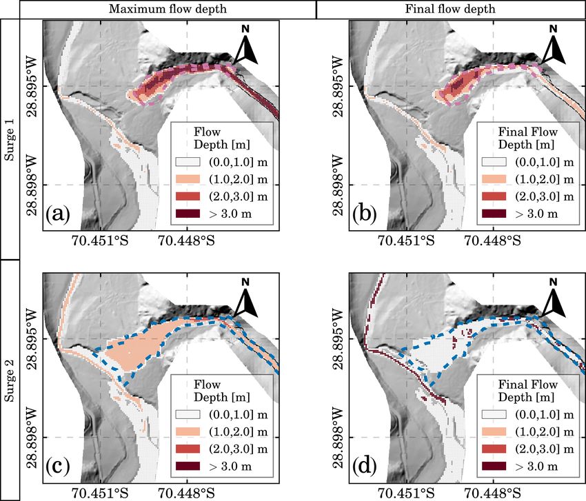
380                    A. Garcés et al.: A modeling methodology to study the tributary-junction alluvial fan connectivity

trimmed the alluvial fan toe (Cabré et al., 2020a), disrupt-
ing the alluvial fan gradient (Fig. 1b). The difference in el-
evation between the main river and the alluvial fan surface
was 13.5 m. This geomorphic configuration promotes the fan
entrenchment and the formation of new fan lobes at its toe
during debris flow events. These lobes may act as barriers
because the valley is narrow (200–300 m wide).
   A post-event topography of a 51 km long segment of the
El Carmen River valley was acquired with 1 m × 1 m hori-
zontal resolution between February and March 2017 by the
Chilean Ministry of Public Works as part of a debris flow
mitigation project in the area (IDIEM, 2019). The vegetation
and buildings were removed from this available topography.
Figure 1a shows the river segment where the Crucecita Alta
fan is located. In the pre-event satellite imagery, retrieved
from © Google Earth Pro v.7.3.3.7786 (CNES/Airbus im-
ages), there is no evidence of a feeder channel connecting
the fan apex with the main river.
   A calibrated HEC-HMS hydrological model (USACE,
2015) of the entire El Carmen River basin is also avail-
able from the same mitigation project (IDIEM, 2019; Zegers
et al., 2020). Water flow discharge at the catchment outlet
and at the river before the junction was obtained from this
hydrological model. The obtained hydrograph shows that the
flood event consisted of four main surges, with a maximum
peak flow of ∼ 7 m3 s−1 during the fourth surge (Fig. 2b).
                                                                   Figure 2. Available data for the 25M event in Crucecita Alta allu-
2.2   Characteristics of the 25M event                             vial fan. (a) The facies F1 (magenta), (b) F2 (blue), (c) F3 (green),
                                                                   and (d) F4 and F5 (orange) retrieved from Cabré et al. (2020a) and
                                                                   lidar topography surveyed by IDIEM (2019). (e) Flow hydrograph
There has been a consensus that storms like the 25M event          obtained from the hydrologic model performed by IDIEM (2019).
in the Atacama Desert occur once a century (Ortega et al.,         The colors used to identify the facies in (a–d) depict their correla-
2019). About the magnitude of the event, Aguilar et al.            tion with the surges in (e).
(2020) estimated the mean erosion rate of the Huasco basin
during the 25M event to be equal to 1.3 mm for the entire
catchment. On the other hand, Aguilar et al. (2014) esti-
mated erosion rates of 0.03–0.08 mm yr−1 during the last 6–        posited sediment volume (Aguilar et al., 2020). The sediment
10 Myr for the same catchment. Assuming that an event such         deposition occurred in a narrow area in the upper portion of
as the 25M event occurs once a century, we can say that the        the fan without reaching the main river. F2 is a wider but
25M event has a “high magnitude” because this single event         less thick deposit (10–30 cm) that overlays F1 and covers all
contributed from 15 % up to 40 % of the total sediment vol-        the fan’s length, from the apex to the distal toe, with nearly
ume eroded, on average, every 100 years.                           5000 m3 of deposited sediment volume (Aguilar et al., 2020).
   Cabré et al. (2020a) characterized the flood event sedimen-     F1 and F2 deposits overlay pre-event sediments, indicating
tology and spatial distribution of the five detected deposits in   that the associated flows had no or negligible erosion capac-
the Crucecita Alta alluvial fan. These deposits were mapped        ity (Cabré et al., 2020a).
and classified into facies (Fig. 2a). The different facies were       Following facies were formed by inertial debris flows.
named from F1 to F5, in which F1 was the first deposit during      These flows can be subcategorized into debris floods, which
the storm, and F5 was the last one. “Sedimentary facies” or        are water-driven floods with high bedload transport of gravel
“facies” is a concept widely used in sedimentological stud-        to boulder-size material in which erosion and sedimentation
ies because it assists in summarizing the grain shape, tex-        processes become important (Church and Jakob, 2020). The
tural parameters, the relief, and the stratification type onto     debris flood surges generated the F3, F4, and F5 deposits and
a single area or zone that can be mapped (Wells and Har-           were responsible for the alluvial fan entrenchment and conse-
vey, 1987). As described by Cabré et al. (2020a), F1 and           quent generation of the feeder channel (Fig. 2b). F3 deposits
F2 correspond to debris flow deposits associated with matrix-      are associated with cohesionless transitional flows (Cabré
supported flows with high fine sediment concentrations. F1 is      et al., 2020a). These flows were channelized below the mid-
the thickest deposit (above 1 m) reaching near 7000 m3 of de-      dle portion of the fan and formed the feeder channel. During

Nat. Hazards Earth Syst. Sci., 22, 377–393, 2022                                     https://doi.org/10.5194/nhess-22-377-2022
A. Garcés et al.: A modeling methodology to study the tributary-junction alluvial fan connectivity                              381

the formation of F3, sediment deposition mainly occurs in the
fan’s upper part and after the fan toe in the El Carmen river.              τy   KηV     n2td V 2
                                                                    Sf =       +       +                                        (3)
After this phase, more dilute flows erode the previously de-               γm h 8γm h2    h4/3
posited materials and enable the deposition of F4 and F5 fa-        In Eq. (3), τy is the yield stress, γm the specific weight of
cies further downstream. Feeder channel depth ranges from           the solid–liquid mixture, h the element (cell) flow depth, K a
100 to 350 cm in the mid zone and reaches up to ∼ 500 cm in         resistance parameter for laminar flow, η the dynamic viscos-
the fan toe (distal zone). The local base level, controlled by      ity of the fluid phase, V the element (cell) flow velocity, and
the main river, was reached during the incision. Therefore,         ntd a pseudo-Manning coefficient corrected by the sediment
the subsequent flows were deposited in a new lobe at the            concentration. O’Brien and García (2009) suggest the fol-
fan toe, exhibiting a telescopic-like morphology with open          lowing empiric relationships, Eq. (4), for estimating the pa-
framework boulders and lobate gravel lenses. These deposits         rameters η, τy , and ntd as functions of sediment volume con-
correspond to inertial debris flows with clast-supported fab-       centration, CV (O’Brien et al., 1993; O’Brien and García,
rics and a matrix-free top (Cabré et al., 2020a).                   2009).
   In our analysis of the 25M event, the cross-cutting rela-
tionships of the facies mapped in Crucecita Alta by Cabré           η = α1 eβ1 CV
et al. (2020a) (F1 to F5) are fundamental evidence to deter-
                                                                    τy = α2 eβ2 CV
mine the sequence of flows. Cabré et al. (2020a) interpret the
significance of the mechanical classification of debris flows       ntd = nbemCV ,                                              (4)
and classify F1 and F2 as non-Newtonian flows. In contrast,
                                                                    where α1,2 and β1,2 are empirical coefficients that have to
F4 and F5 are classified as Newtonian flows, which is a sim-
                                                                    be calibrated, n is the conventional Manning coefficient, b =
ilar differentiation, to some extent, to the viscous and inertial
                                                                    0.0538, and m = 6.0896.
debris flow classification of Takahashi (2014). F3 is a transi-
                                                                       The model also used a detention coefficient (SD) that con-
tional flow between the observed non-Newtonian and New-
                                                                    trols flow detention. D’Agostino and Tecca (2006) suggest
tonian flows.
                                                                    that SD works as a minimum physically plausible flow depth.
                                                                    In addition, Zegers et al. (2020) reported that SD is one of the
3     Methodology                                                   two more sensitive parameters in the model, and, even though
                                                                    it is not part of the rheological model, it can be a surrogate
3.1    Governing equations                                          for the flow rheology.
                                                                       FLO-2D is also capable of solving sediment transport
We use the two-dimensional FLO-2D model to solve the                equations to simulate mobile bed and topographic adjust-
flood wave progression for water and debris flows in complex        ments. In the FLO-2D model, the coupling of the sediment
topographical terrains (O’Brien and García, 2009). FLO-2D           transport computation and the flow hydraulics are solved in a
solves two-dimensional depth-averaged continuity and mo-            two step procedure; i.e., water flow characteristics are com-
mentum equations, Eqs. (1) and (2), known as Saint-Venant           puted first, and then sediment transport and bed geometry
equations, for water and debris flows.                              changes, due to sediment erosion or deposition, are computed
                                                                    for that time step (O’Brien and García, 2009). However, no
∂h ∂hVx ∂hVy                                                        erosion/deposition processes can be included when using the
    +       +      = 0,                                      (1)
∂t     ∂x      ∂y                                                   mudflow module.
            ∂h Vx ∂Vx Vy           ∂Vx 1 ∂Vx                           The sediment transport model accounts for the local
Sfx = S0x −    −        −              −
            ∂x    g ∂x    g         ∂y   g ∂t                       deficit/excess of transported sediment, modifying the bed
            ∂h Vx ∂Vy Vy           ∂Vy 1 ∂Vy                        channel height using the well-known Exner equation, Eq. (5).
Sfy = S0y −    −        −              −      ,              (2)
            ∂y    g ∂x    g         ∂y   g ∂t                                        ∂qsx ∂qsy

                                                                    ∂h0        1
                                                                          +                +        =0                           (5)
where h is the flow height, Vx and Vy are flow velocities             ∂t     1 − p ∂x          ∂y
in the x and y directions, and S0x and S0y are the channel          In Eq. (5), h0 is the height of the channel bed, qs is the sedi-
slopes in each transverse direction (x, y). Sfx,y denotes the       ment load, and p is the porosity. For the sediment load (qs ),
frictional slope, accounting for flow resistance. In the case of    FLO-2D has 11 different expressions based on unique river
water flows, Sfx,y is calculated using the Manning equation.        conditions (O’Brien and García, 2009). For this study, we
In the case of mudflows, Sfx,y is calculated using the so-called    used the Parker–Klingeman–Mclean equation (Parker et al.,
quadratic rheology model, Eq. (3), which combines different         1982), Eq. (6). This equation is suitable for gravel and sandy
terms accounting for yield and coulomb, viscous, and turbu-         bed material and simulates sediment transport mechanisms
lent and dispersive stresses (O’Brien and García, 2009).            from bedload to mixed suspended sediment loads.
                                                                           W ∗ u3∗ ρs
                                                                    qs =              ,                                         (6)
                                                                           (s − 1)g

https://doi.org/10.5194/nhess-22-377-2022                                      Nat. Hazards Earth Syst. Sci., 22, 377–393, 2022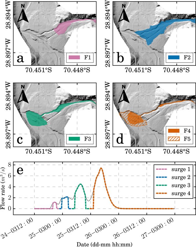
382 A. Garcés et al.: A modeling methodology to study the tributary-junction alluvial fan connectivity
Figure 3. Topographic data modifications. Post-event topography corresponds to the available lidar topography while the pre-event topog-
raphy is a restitution based on satellite images and the available topography. The synthetic channel (dashed brown line) attached to the lidar
topography is 550 m long, while feeder channel (dashed orange line) is 450 m long. In the post-event topography, the feeder channel is the
result of the inertial debris flow incisions on the alluvial fan. In the mitigation works’ topography, the feeder channel was replaced by a
straight rectangular channel.
where W ∗ is √the dimensionless sediment transport rate,
Eq. (7), u∗ = τ0 /ρ the frictional velocity, τ0 the bottom (D30 )2
shear stress, ρs the density of the sediments, ρ the water den- SCC = (10)
D10 D60
sity, s = ρs /ρ the specific weight, and g the gravitational ac-
celeration. Cabré et al. (2020a) reported that viscous debris flows ob-
served in the Crucecita Alta fan show negligible erosion.
W∗ = Therefore, the mudflow model of FLO-2D is enough to rep-
4.5
resent the flow characteristics of viscous debris flows. On the
0.822
11.2 1 −
φ50 φ50 > 1.65
0.0025 exp 14.2 (φ50 − 1) − 9.28(φ50 − 1)2
0.95 ≤ φ50 ≤ 1.65 , other hand, Cabré et al. (2020a) indicate that inertial debris
14.2 flows observed in the Crucecita Alta fan significantly modi-
0.0025φ50 φ50 < 0.95
(7) fied its morphology, so erosion and deposition processes can
not be neglected. Since FLO-2D can not use the mudflow
where φ50 is the normalized Shields stress, also known as and sediment transport models simultaneously, we used the
transport stage, Eq. (8). following reasoning. For viscous debris flows, the first two
τ50∗ terms of Eq. (3), i.e., yield and viscous stresses, dominate
φ50 = flow resistance. Conversely, for inertial debris flows, the third
τr∗50
term of Eq. (3), i.e., turbulent and dispersive stresses, be-
∗ u∗2 comes more important for estimating Sf . Because of this be-
τ50 = , (8)
(s − 1)gD50 havior, inertial debris flows can be modeled using the same
where τ50∗ is the Shields stress, τ ∗ = 0.0876 is a reference Manning approach for water flows but considering an ap-
r50
Shields stress value, and D50 is the mean sediment size of propriate Manning coefficient. This approach has been val-
the substrate. idated in previous studies, in which the Manning coefficient
Originally, Eq. (7) considered W ∗ = 0 for φ50 < 0.95, but was estimated by back-calculation (Rickenmann et al., 2006;
it was modified by Parker (1990) to have a positive trans- Naef et al., 2006). Typically used values for the Manning co-
port rate in every flow condition. Parker and Klingeman efficient for modeling turbulent Newtonian debris flows are
(1982) did another modification for multiple sediment sizes, around 0.1 (Rickenmann, 1999).
in which the dimensionless fractional transport rate Wi∗ for
3.2 Model configuration
diameter Di is calculated as a function of Eq. (9).
∗
τ50 D50 0.018
The FLO-2D model built for this tributary-junction alluvial
φi = ∗ (9) fan considers a 1400 m long river section and a 450 m long
τr50 Di
section of the alluvial fan, from the fan apex to the river
The FLO-2D model allows the user to specify the sediment junction (Fig. 3). To have an adequate flow development and
gradation coefficient, SCC , Eq. (10), which is a metric of the achieve the balance of the sediment transport capacity before
sediment size distribution. reaching the fan apex, the lidar topography of Crucecita Alta
Nat. Hazards Earth Syst. Sci., 22, 377–393, 2022 https://doi.org/10.5194/nhess-22-377-2022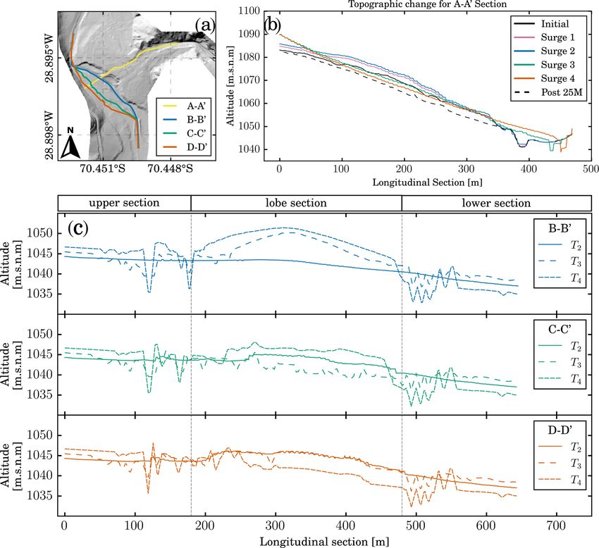
A. Garcés et al.: A modeling methodology to study the tributary-junction alluvial fan connectivity                                 383

was extended 550 m upstream using the ALOS PALSAR
DEM (digital elevation model) (12.5 m × 12.50 m resolution:
© JAXA/METI ALOS PALSAR L1.0 2007). Secondly, be-
cause the ALOS PALSAR topography does not have the res-
olution to represent the creek topography, a synthetic chan-
nel was created in the extended zone to better represent the
channel morphology. The synthetic channel dimensions were
mapped based on the Google Earth Pro scenes. Thus, the
model is 1 km long from the Crucecita Alta catchment (from
the inflow element to the river junction), where 450 m cor-
responds to the lidar topography and 550 m to the synthetic
channel (Fig. 3). No pre-event high-resolution topography is
available for the Crucecita Alta fan. This is a common prob-
lem when studying the geomorphic consequences of low-
frequency, high-magnitude debris flow events in arid areas
(Zegers et al., 2017). To overcome this limitation, similarly to
the approaches used by McMillan and Schoenbohm (2020),
the post-event raster was modified to reproduce the pre-event
topography based on available pre-event imagery and field
evidence. The pre-event geomorphological configuration of
the Crucecita Alta fan (Fig. 3) consists of an undisturbed fan
surface without evidence of erosion (caused by the incision
of a feeder channel or headward erosion). The modifications
performed over the post-event lidar topography to obtain the
pre-event geometry can be summarized into the following:
(i) the incisions caused by the 25M flood event in the alluvial
fan were removed from the DEM, and then the surface was            Figure 4. Surge modeling workflow. The main challenge is to find
smoothed; and (ii) facies F1 and F2 were subtracted from the       a correlation between surges and field data that allows the user to
DEM based on field thickness measurements of the deposits          discriminate between viscous and inertial debris flow surges. The
and assuming that cohesive debris flows have little to negli-      developed routine is able to concatenate the surges by updating the
gible bed erosion (Cabré et al., 2020a).                           model inputs for the next surge, based on the results of the previous
   We also study the effects that a bypass channel, a typi-        one.
cal debris flow mitigation work in alluvial fans, has on the
fan–river connectivity. To this purpose, a 10 m wide and 10 m
deep rectangular channel was inserted in the pre-event topog-      bris flows mainly deposited sediments in the fan surface. In
raphy (Fig. 3).                                                    contrast, inertial debris flows strongly incised and eroded the
   The resolution of the numerical grid was set at 5 m × 5 m,      fan. Consequently, our modeling approach divides the debris
as a finer resolution results in numerical instabilities due to    flow event between viscous and inertial debris flow surges
the high flow velocities. In contrast, a coarser grid resolu-      and correlates them to the field evidence (Fig. 2). Therefore,
tion results in a loss of terrain information. Manning num-        if the facies (or any other sedimentological description) indi-
ber, n, was set equal to 0.1 s m−1/3 for the alluvial fan, which   cates that a viscous debris flow formed the deposit, the asso-
is within the range suggested by Rickenmann et al. (2006)          ciated surge is modeled with the mudflow model. Conversely,
(0.07–0.16 s m−1/3 ) for debris flows. Although the incisions      if the facies suggests an inertial debris flow, the surge is com-
measured in the field reach up to 5 m deep, erosion depth was      puted using the water flow model with n = 0.1 and including
limited to 4 m as greater depths affect the model stability. No    sediment transport. For this purpose, we developed a Python
sediment rating curve was set for the inlet because the 550 m      routine to concatenate the four surges into one model. Each
synthetic channel allows the model to find its own sediment        surge is modeled in a sequence in which the results of the
load equilibrium before reaching the fan apex.                     previous surge modify the topography for the next surge. The
                                                                   workflow steps are presented in Fig. 4.
3.3   Modeling approach and workflow                                   In the first step of this workflow, “subdivision into surges”
                                                                   (Fig. 4), we set the number of surges i = 1 . . . N and the
The flood sequence of the 25M event consisted of four dif-         rheology model of each one, i.e., non-Newtonian (viscous
ferent debris flow surges with different sediment loads. The       debris flow) or Newtonian (inertial debris flow). For exam-
differences in the rheology of the flows resulted in multiple      ple, facies F1 and F2 have high fine sediment concentration,
geomorphological adjustments within the fan. Viscous de-           present evidence of a laminar flow, and show negligible ero-

https://doi.org/10.5194/nhess-22-377-2022                                    Nat. Hazards Earth Syst. Sci., 22, 377–393, 2022
384                          A. Garcés et al.: A modeling methodology to study the tributary-junction alluvial fan connectivity

sion. Therefore, surges 1 and 2 are assigned as viscous debris        a reduction from seven to four parameters in the calibration
flows. In contrast, the following surges 3 and 4 are assigned         process). Parameters α1 and α2 were fixed since they are the
as inertial debris flows since F3, F4, and F5 show significant        least sensitive parameters of the model (Zegers et al., 2020)
erosion and deposition and consist primarily of coarse sedi-          and were set equal to 0.0075 poises and 0.152 dynes per
ment.                                                                 cubic centimeter, respectively, using the values obtained by
   For the mudflow branch of the workflow (Fig. 4) the next           Zegers et al. (2017). Conversely, the SD parameter has a con-
step is the “calibration process and result screening”. This          siderable influence on the results (Zegers et al., 2020). This
step finds the best set of rheological parameters, as explained       parameter sets a minimum physically plausible flow depth,
in the next section. Multiple model runs may pass the screen-         allowing the mixture to stop on the alluvial fan (i.e., the mud-
ing. Therefore, in the step “model selection”, the user must          flow stops if the local flow depth is lower than SD). Based
visually inspect all the filtered runs and choose the best fit for    on estimated deposit height measurements by Cabré et al.
the characterized facies. This step could not be automated be-        (2020a), we tested different values for SD to reproduce the
cause a critical analysis is needed. From the selected run, the       event by trial and error. SD was finally set equal to 1 m for
deposit depth hd is estimated for each grid element according         the alluvial fan and 0.03 m for the river valley, in which the
to Eq. (11), where hf is the resulting final flow depth reported      value in the valley is the default value in FLO-2D for water
by the numerical model, and CVmean is the mean volumetric             flows.
concentration of the surge. The sediment rating curve func-              We used the algorithm of Zegers et al. (2020) as the basis
tion CV (Q, t) is presented in Zegers et al. (2020). Porosity p       to develop a novel decision support system (DSS) that allows
is set equal to 0.3 for facies F1 and F2 (Nicolleti and Sorriso-      us to run the model N times and automatically apply screen-
Valvo, 1991). Finally, hd is added to the original topography         ings to determine the model’s best fit. Zegers et al. (2020)
at each cell by the Python routine, which updates the model           found that the calibration by flood area and deposited volume
for the next surge.                                                   also constrained the flow velocity and flow height. Therefore,
                                                                      our DSS has incorporated filters for the affected area and the
          CVmean
hd = hf                                                               deposited volume. Similar to Mergili et al. (2018), we as-
          1−p                                                         signed the pixels within the observed deposit as observed
             RT                                                       positives (OPs) and pixels outside the deposit area as ob-
                   Q(t)CV (Q, t)dt                                    served negatives (ONs). The pixels flooded by the simulation
             t=0
CVmean   =                                                    (11)    were assigned as predicted positives (PPs), whereas the non-
                    RT
                         Q(t)dt                                       flooded pixels were assigned as predicted negatives (PNs).
                   t=0                                                Hence, the screenings filter the results based on thresholds θ1
   For the sediment transport model branch of the workflow            and θ2 associated with true positives (TP = OP ∧ PP) and
(Fig. 4), on the other hand, the model is directly run since          false positives (FP = ON ∧ PP) (Eq. 12). The aim of this
no parameters need to be calibrated. The sediment transport           thresholds is to find a manageable amount of filtered runs
model only needs the parameters D50 and SCC (Eq. 10) of the           for visual inspection rather than finding specific threshold
substrate. In Crucecita Alta alluvial fan, D50 = 7.8 mm and           values. Moreover, these thresholds vary due to the distribu-
SCC = 1.79 (Cabré et al., 2020a). We assumed that the sedi-           tion of the results, even for surges 1 and 2 in the same allu-
ment transport equation and the grain size distribution of the        vial fan. In particular, the affected area thresholds were set
substrate do not change between surges. After running the             equal to θ1 = 0.7 and θ2 = 0.3 for surge 1 and θ1 = 0.9 and
sediment transport model, our routine updates the model to-           θ2 = 0.1 for surge 2. The deposited volume threshold was set
pography according to the computed erosion and deposition             as ±60 % of the deposited volume estimated from field ob-
for each pixel; this updated topography is used for simulating        servations for both surges.
the next flow surge.                                                   P TP
                                                                          pxi
                                                                                        P FP
                                                                                           pxi
                                                                      P OP > θ1 P OP              < θ2                             (12)
3.4   Decision support system (rheology calibration)                      pxi              pxi

Zegers et al. (2020) performed a sensitivity analysis for the            For the selected parameters, we choose the range of each
FLO-2D numerical model and established the most sensitive             parameter based on the ranges defined by Zegers et al.
parameters in the mudflow model. In their study, two allu-            (2020). To generate the combination of parameters for each
vial fans located in the same valley were tested. They con-           simulation, we used the Latin hypercube sampling (LHS)
cluded that equifinality was present in the model, mainly             method (Olsson and Sandberg, 2002). Since we simulated
related to the rheological parameters. Thus, to reduce over           surges 1 and 2 with the mudflow model, both surges needed
parameterization and restrict the parameter search, three pa-         a calibration process to find their rheological parameters. We
rameters (α1 , α2 , and SD) have been left out of the calibra-        tested the model with sets of 50, 100, and 200 runs. Due to
tion process. Consequently, the calibrated parameter set cor-         the constraint of calibrated parameters from seven to four,
responds to the parameters β1 , β2 , CVmax , and Volsediment (i.e.,   100 model runs were sufficient to find reasonable results that

Nat. Hazards Earth Syst. Sci., 22, 377–393, 2022                                       https://doi.org/10.5194/nhess-22-377-2022
A. Garcés et al.: A modeling methodology to study the tributary-junction alluvial fan connectivity 385
Figure 5. Viscous debris flow surges. Panels (a, b) correspond to the results for surge 1, whereas panels (c, d) correspond to the results for
surge 2. Dashed polygons show the extent of mapped facies F1 (blue) and F2 (red). Panels (a, c) present the maximum flow depth, whereas
panels (b, d) present the final flow depth at the end of each surge. Topographic changes for subsequent surges are updated based on the final
flow depth of the previous surge.
Table 1. Calibrated parameters and their range for surges 1 and 2. 4 Results
Parameters for both surges were expected to be different because of
the equifinality and their different sedimentologic characteristics. In this section, we analyze if the proposed workflow can re-
produce the debris flow event and the geomorphological ad-
β1 β2 max
CV VolSediment [m3 ] justments that this alluvial fan experienced. Once the work-
Surge 1 Surge 2 flow capabilities are proven, we include a rectangular chan-
nel that connects the alluvial fan apex with the river. This
Min 6.00 17.00 0.45 4000 3000
Max 33.00 30.00 0.60 10 000 7000 channel is tested for the same chain of debris flow surges as
Calibrated surge 1 20.23 17.20 0.58 9482 – in the 25M event and also for two inertial debris flow surges.
Calibrated surge 2 18.14 20.55 0.50 – 4167 Then, we study the effect of this channel on the lateral and
longitudinal coupling status of the river junction.
fit the mapped deposits. For 50 runs, no result fits the screen- 4.1 The 25M debris flow event reconstruction
ings, whereas 200 runs show no significant improvements.
The screenings applied, Eq. (12), returned four cases for each The maximum and final flow depths of the viscous debris
surge which were visually inspected to select the best fit. flow surges 1 and 2 are presented in the flood inundation
Considering the modified topography after the selected case maps of Fig. 5. In a first visual inspection of Fig. 5, the
for F1, we ran the same algorithm for the second surge. The simulated flooded areas are in good agreement with the fa-
minimum and maximum values for the calibrated parameters cies mapped. Integrating the inflow hydrograph and con-
and the parameters adopted for surges 1 and 2 after the cali- sidering the variable CV , for surge 1, the inflow volume is
bration process are presented in Table 1. 15 450 m3 of water and 16 991 m3 of sediment resulting in
CVmean = 0.52. According to the simulation, the volume of
sediment deposited on the alluvial fan is 9482 m3 (Fig. 5a
and b). In contrast, the volume estimated from field measure-
https://doi.org/10.5194/nhess-22-377-2022 Nat. Hazards Earth Syst. Sci., 22, 377–393, 2022386 A. Garcés et al.: A modeling methodology to study the tributary-junction alluvial fan connectivity Figure 6. Inertial debris flow surges. Panels (a, b) correspond to the results for surge 3, whereas panels (c, d) correspond to the results for surge 4. Dashed polygons delimit the telescopic-like deposit, i.e., the incision in the alluvial fan and the new lobe at the fan toe. Pan- els (a, c) present the maximum flow depth, while panels (b, d) present the topographic change for erosion (negative values) and deposition (positive values). ments is ca. 7000 m3 (F1). The integration of the inflow hy- We expected this condition because the simulated deposited drograph for surge 2, on the other hand, results in an inflow volume is very sensitive to SD when the alluvial fan oper- volume of 28 218 m3 of water and 10 453 m3 of sediment, ates as a buffer preventing sediments from reaching the river i.e., CVmean = 0.27. The lower value for CVmean for surge 2 in- (Zegers et al., 2020). However, SD = 1 m overestimates the dicates a lower flow resistance than surge 1. According to sediment deposit thicknesses for surges 1 and 2. We also the simulation, the deposited sediment volume is 4167 m3 tested lower SD values of 0.5 and 0.7 m, associated with (Fig. 5c and d), whereas the volume estimated from field deposit thicknesses of 0.2 and 0.3 m according to Eq. (11), measurements is 5000 m3 (F2). obtaining unsatisfactory results regarding the observed af- Surge 1 does not reach the river due to its high CVmean fected area. The problem with lower SD values is that the and the absence of a channel (Fig. 5b). In a fan without a flow spreads over the surface, losing any correlation with the feeder channel, viscous flows spread over the surface, in- mapped facies. Therefore, we prioritize matching the flooded creasing flow resistance and promoting flow detention and area instead of the deposit thickness for the model calibration consequent sediment deposition (Jakob and Hungr, 2005). as measuring the flooded area is more reliable than charac- Surge 2 reaches the river (Fig. 5d) probably given to its more terizing the deposit thickness distribution. diluted nature (lower CVmean than surge 1). Thus, a small por- Our simulation results for the following inertial debris tion of the sediment transported by surge 2 reaches the river, flow surges 3 and 4 are presented in Fig. 6. These surges have but it was insufficient to change the river geometry. There- a higher amount of water than the previous viscous surges. fore, the alluvial fan acts as a sediment buffer, preventing the Surge 3 has a total volume of water of 61 388 m3 and surge 4 interaction with the main river. Consequently, the river’s sed- of 143 568 m3 . The maximum flow depth maps of Fig. 6a iment discharge remains almost undisturbed even with the and c are evidence of the river avulsion triggered by surge 3, occurrence of surges 1 and 2. where the original river path and the newly formed river path The SD parameter controls the flow depth at the end of are observed. The river is pushed to the opposite valley side the simulation for the viscous debris flow surges and, conse- due to surge 4 with flow depths over 2 m deep. The result- quently, their resulting deposit thicknesses (Fig. 5b and d). ing topographic changes for surges 3 and 4 (Fig. 6b and d) Nat. Hazards Earth Syst. Sci., 22, 377–393, 2022 https://doi.org/10.5194/nhess-22-377-2022
A. Garcés et al.: A modeling methodology to study the tributary-junction alluvial fan connectivity                             387

are coherent with the primary erosion and deposition zones         sections (Fig. 7a). All longitudinal profiles are presented in
identified during fieldwork. Moreover, it is possible to locate    the downstream direction. We established the A-A’ profile
the new lobe formed at the fan toe showing a telescopic-like       of the alluvial fan according to the main incision observed
pattern responsible for the river avulsion and the partial river   in the field after the 25M event. In contrast, sections B-B’,
blockage. On the other hand, the new scoured channel on the        C-C’, and D-D’ correspond to the main river, which shifted
alluvial fan is wider than the channel observed in the field       during the event.
possibly due to the numerical model resolution. These re-             River avulsion is well defined in profile A-A’ (Fig. 7b),
sults show that the fan–river interactions become important        where the river channel shifts to the opposite valley side after
for surges 3 and 4 because the tributary sediment discharge        surges 3 and 4 due to the formation of a new lobe. Profile A-
experiences a complete coupling with the main river through        A’ shows a convex shape after surge 1, typical for viscous
alluvial fan trenching and progradation. Savi et al. (2020) re-    debris flows with sharp frontal boundaries. The following
ported similar behavior in their laboratory experiments.           surge 2 stacks over surge 1, maintaining this convex shape
   We also analyzed the potential river blockage or dam for-       and raising the topography. On the other hand, inertial de-
mation. The obstruction ratio represents the space occupied        bris flow surges 3 and 4 result in a characteristic concave
by sediment deposits compared to the available space for the       shape for profile A-A’ due to an alluvial fan incision. Ana-
river to flow (Stancanelli and Musumeci, 2018). This ratio is      log laboratory experiments of Savi et al. (2020) reproduced
useful to discriminate between three states (no blockage, par-     similar sediment mobilization and geomorphic changes. The
tial blockage, full blockage). The obstruction ratio rb is de-     results of our simulation show less scour than the observed
fined as the ratio between the obstruction lobe width and the      incision in the field possibly because of the fixed 4 m of max-
flooded valley width, both along the orthogonal direction to       imum erosion. Another explanation for the lack of erosion is
the river flow (Stancanelli and Musumeci, 2018). The value         the difference between eroding the early event deposits (F1
rb = 1 means a complete river blockage. River blockage or          and F2) and the pre-event old debris flow deposits. In our rou-
dam formation is dominated by the momentum ratio RM and            tine, the new deposits are accounted part of the topography
the unevenness of the grain sizes SC (Dang et al., 2009). The      instantly when our routine updates the topography between
momentum ratio is calculated as the product of the flow rate       surges. However, the early event sediments should be eroded
ratio RQ , the velocity ratio RV , the bulk
                                        √ density ratio Rγ , and   easier than old pre-event deposits.
the confluent angle θ , while SC = D75 /D25 . Dang et al.             The B-B’ profile follows the river channel observed in
(2009) proposed a critical index C = RM SC for dam for-            the lidar topography. Profile C-C’ corresponds to the main
mation with different partial and complete blockage thresh-        flow path of the river after the new lobe associated with
olds. Stancanelli and Musumeci (2018) highlighted that the         surge 3. Profile D-D’ corresponds to the main final flow path
thresholds have to be calibrated depending on the material         at the end of surge 4 and, therefore, at the model’s end.
adopted. For gravel deposits, they proposed a threshold value      The upper and lower sections are the same for these three
of C = 9.                                                          profiles, whereas the lobe section follows the river avulsion
   For surges 3 and 4, we obtained C indexes of 2.15               path. Therefore, profiles B-B’, C-C’, and D-D’ are presented
and 0.85, respectively. These values indicate that both surges     for T2 , T3 , and T4 , which correspond to the status of the main
do not have the potential to block the river. The C indexes        channel after surge 2, 3, and 4, respectively (Fig. 7c). Ini-
are consistent with the obstruction ratios rb of 0.75 (surge 3)    tial status and the status of the river after surge 1 remain the
and 0.86 (surge 4). These rb values indicate a river’s partial     same as T2 and are not presented here. Profile B-B’ illustrates
blockage due to the lateral input of sediment. Interestingly,      how the sediment yielded from the tributary reaches the river
the river experiences deposition in its downstream section for     forming the new lobe of the telescopic-like deposit with max
surge 3, i.e., an excess of sediment load (Fig. 6b). Conversely,   deposited depths around 6 m for T3 and 4 m for T4 . Surge 3 is
the river experiences erosion in the downstream section for        responsible for the first channel avulsion, represented in the
surge 4, i.e., a deficit of sediment load (Fig. 6d). This change   C-C’ profile for T3 , and is evidence of the new lobe extent.
indicates that a river obstruction rb = 0.75 was not able to       Surge 4 increases the fan progradation, so profile C-C’ ex-
act as a barrier. In contrast, an obstruction ratio rb = 0.86      hibits deposition for T4 in the lobe section. During surge 4,
was able to act as a barrier decoupling the river’s sediment       the river shifts again, and the D-D’ profile follows the final
discharge in the river junction. For both inertial surges, the     river path where T4 is evidence of the erosion and formation
upper section of the river is a deposition zone because of the     of the final river path.
river’s partial obstruction and, consequently, pounded water.
                                                                   4.3   Simulation of different scenarios considering
4.2   Morphological evolution of the tributary-junction                  mitigation works
      alluvial fan
                                                                   In hazard assessment projects, numerical models are also
We characterized the tributary-junction alluvial fan evolution     used to design mitigation works. However, these models do
by analyzing the topographic change using four longitudinal        not always consider the broad debris flow types that a creek

https://doi.org/10.5194/nhess-22-377-2022                                   Nat. Hazards Earth Syst. Sci., 22, 377–393, 2022
388 A. Garcés et al.: A modeling methodology to study the tributary-junction alluvial fan connectivity
Figure 7. Morphological evolution of the tributary-junction alluvial fan. (a) Location of the longitudinal sections presented in (b) and (c).
(b) Longitudinal profile A-A’ of the alluvial fan topography after each surge. (c) Longitudinal profiles B-B’, C-C’, and D-D’ of the river’s
topographic evolution.
can experience. Moreover, the same hydraulic works should portion of the fan. We first tested channels with smaller cross-
be studied under the broad flow typology. As an example, we sections where overflow also occurred, whereas a larger
tested a rectangular channel (10 m width and 10 m depth) that channel cross-section would be cost-inefficient and, there-
connects the alluvial fan apex with the river junction under fore, not realistic.
two different scenarios: (1) Scenario 1 consists of the same This case shows that a channel is not sufficient to con-
sequence of debris flow surges observed in the 25M event, in vey the debris flows safely. However, deposits observed in
which two viscous debris flows are followed by two inertial the river junction are smaller than deposits observed in the
debris flows. (2) Scenario 2 consists only of the two inertial original case. Surprisingly, the presence of a channel does
debris flows. With both scenarios, we prove the importance not directly mean an increase in lateral connectivity. In the
of studying different debris flow type combinations for the 25M event, alluvial fan trenching creates a local increase in
same mitigation work. the sediment load, which is immediately deposited at the fan
toe due to the change in the slope. From this test, we learned
4.4 Scenario 1 two important features when assessing this debris flow haz-
ard. First, trimmed fan toes create a base level drop that in-
In Scenario 1 (Fig. 8a–d), the proposed channel confines vis- creases the sediment load that reaches the river, enhancing
cous debris flows, which allows the flow to reach the river river avulsion. Second, transport-limited catchments such as
for surges 1 and 2. For surge 1 (Fig. 8a), deposit depth in Crucecita Alta produce sediment discharges during extreme
the channel is up to 7 m and over the river junction up to storm events, resulting in cost-inefficient works which are
4 m, indicating a partial channel obstruction. Surge 2, on the not realistic. To sum up, channels may reduce the impact
other hand, spreads over the river junction but does not form of debris flows, but they do not entirely solve the problem.
a new lobe. Surges 3 and 4, shown in Fig. 8c and d, are de- Therefore, targeted population education to avoid people set-
viated and forced to deposit due to the previous deposits. tling in areas at risk must join these works.
With surge 4, avulsion is present, inundating the southern
Nat. Hazards Earth Syst. Sci., 22, 377–393, 2022 https://doi.org/10.5194/nhess-22-377-2022A. Garcés et al.: A modeling methodology to study the tributary-junction alluvial fan connectivity 389
Figure 8. Two future scenarios are modeled to understand the possible effects of a channel (mitigation works): first scenario (a–d) and second
scenario (e, f).
4.5 Scenario 2 scenario, only a mild river avulsion without river obstruction
occurs for surge 3 and surge 4.
Scenario 2 (Fig. 8e and f), consisting of two inertial debris
flow surges, also demonstrates that the presence of a chan- 5 Discussion
nel avoids the telescopic-like deposit. The channel avoids an
abrupt base level drop due to the trimmed fan toe and, there- 5.1 Dynamic response of the fan–river connectivity
fore, avoids headward erosion and the local increase in sed-
iment load. Consequently, no local sediment load increase The field “forensic” analysis of the debris flow event in the
takes place in the alluvial fan for surges 3 and 4. For this Crucecita Alta fan resulted in a clear differentiation of the
https://doi.org/10.5194/nhess-22-377-2022 Nat. Hazards Earth Syst. Sci., 22, 377–393, 2022390 A. Garcés et al.: A modeling methodology to study the tributary-junction alluvial fan connectivity transport mechanisms for each surge (Cabré et al., 2020a). in lower sediment loads, reducing the size of the new lobe at Our workflow benefits from this differentiation to select a the fan’s toe. The results of scenario 2 (Fig. 8e and f), which specific model to represent the flow of the water–sediment consider only the inertial debris flows, show that the chan- mixture in each surge. Our results show that the combination nel avoids the headward erosion observed in the 25M event. of these numerical models reproduces the main processes Consequently, the amount of sediment deposited at the new described by Cabré et al. (2020a). For the 25M event in lobe at the fan toe is reduced considerably compared to the Crucecita Alta alluvial fan, the coupling conditions changed original case, even though we expected that the presence of within the event, but our workflow can reproduce this dy- the channel would increase the structural connectivity. namic response. For the 25M event in the Huasco basin, Cabré et al. (2020a) reported 49 catchments with a charac- 5.2 Model limitations teristic response in which seven catchments are described in detail. This specific response of the catchments consists of Even though our workflow successfully reproduces the main viscous debris flow surges, followed by inertial debris flow processes of interest, we observed two main limitations. surges. This catchment response in the Atacama Desert also First, we recognize that neglecting bank erosion may af- occurred in 2017 and 2020 but has not been reported yet. fect the sediment cascade dynamics. However, this pro- Characteristic stratigraphic and geomorphic features ob- cess is rarely considered because most numerical models served in the Huasco River basin can also be used to un- do not account for bank erosion. Second, the surface de- derstand changes in the water–sediment ratio and the cou- tention parameter (SD) directly impacts the deposited vol- pling degree between fans and the main river. We observed ume of sediment (Volsediment ) in the calibration process be- in the field that sediment sources influence the fine sedi- cause it controls the final flow depth. Therefore, estimat- ment vs. coarse sediment ratio present in the debris flows. ing the SD parameter based on field data is advisable. If no On the one hand, viscous debris flows travel short distances data of the deposit depth are available to estimate this pa- because of their high flow resistance. Therefore, these surges rameter, SD could be added to our novel decision support come from sources close to the fan apex and arrive first. Con- system. However, we calibrated a parameter set of four un- versely, inertial debris flows can travel longer distances and knowns (β1 , β2 , CV , Volsediment ), whereas considering five come from more distant sources (i.e., they arrive later at the unknowns increases the computational costs exponentially. alluvial fan). We expect this behavior to keep occurring in In the absence of a proper estimation of SD, we recommend these arid zones; therefore, our workflow could be used to that the user chooses a value between 0.5 and 1 m for viscous study future scenarios. Moreover, our workflow could assist debris flows in steep alluvial fans in the Atacama Desert in- in the volume estimations of water and sediment needed to stead of adding SD to the DSS. This will maintain computa- modify the sediment cascade dynamics under viscous and in- tional costs reasonably. The range [0.5, 1] m is based on this ertial debris flows, which are different, as seen in this study. study’s findings and other previous studies in the Atacama Using our workflow on a past event in Crucecita Alta, we Desert, such as Zegers et al. (2017, 2020). Despite these lim- determined the following characteristics. The fan can com- itations, it is shown here that fan–river interaction studies can pletely buffer the viscous debris flow surge 1 (CVmean = 0.52 be performed with a commercially available software appli- and a volume of sediment around 9500 m3 ). Conversely, for cation that simplifies the physics around the flow of solid– surge 2, a still viscous but more diluted debris flow, the fan liquid mixtures. partially buffers the sediment discharge (CVmean = 0.27 and a volume of sediment around 4200 m3 ). Moreover, for both 5.3 Insights for a new modeling approach later inertial debris flows, the sediment discharge of the trib- utary is totally coupled. Alluvial fan trenching for surge 3 High-intensity rainstorm events in the Atacama Desert increases the river’s sediment load downstream, leading to have increased their occurrence in the last century, and it total connectivity of the sediment cascade. Conversely, for is expected that this trend will continue due to climate surge 4, the greater volume of sediment acts as a barrier that change (Ortega et al., 2019). A higher frequency in high- decouples the sediment discharge of the river. intensity rain events in these transport-limited (i.e., sediment- Our methodology is helpful to study hypothetical scenar- unlimited) catchments (Aguilar et al., 2020) results in a ios, such as a channel designed to mitigate affected areas but higher frequency in the debris flow events. Following this increasing the coupling status of the alluvial fan. The results reasoning, the necessity of properly reproducing the debris of scenario 1 (Fig. 8a–d) show that viscous debris flows can flow mechanics should be a priority. Most of the models reach the river since they remain confined to the channel. focus on run-out distance and affected area, but none cope However, sediment deposition occurring during the flow re- with the notorious changes in rheological macroscopic be- duces the channel transport capacity for the following surges. haviors between surges. Based on the data for a specific Thus, when the inertial debris flow surges occur, we observe event, our workflow studies the tributary-junction alluvial that the channel can convey surge 3 but not surge 4. Com- fan’s response to a characteristic chain of flows with differ- pared to the original 25M event, smaller erosion areas result ent rheological behaviors in the arid region of Chile (27– Nat. Hazards Earth Syst. Sci., 22, 377–393, 2022 https://doi.org/10.5194/nhess-22-377-2022
You can also read