Air traffic and contrail changes during COVID-19 over Europe: A model study
←
→
Page content transcription
If your browser does not render page correctly, please read the page content below

Air traffic and contrail changes during COVID-19 over Europe: A
     model study
     Ulrich Schumann1, Ian Poll2, Roger Teoh3, Rainer Koelle4, Enrico Spinielli4, Jarlath Molloy5, George S. Koudis5,
     Robert Baumann1, Luca Bugliaro1, Marc Stettler3, Christiane Voigt1,6
     1
 5     Institute of Atmospheric Physics, Deutsches Zentrum für Luft- und Raumfahrt, 82234 Oberpaffenhofen, Germany
     2
       Emeritus Professor of Aerospace Engineering, Cranfield University, UK
     3
       Centre for Transport Studies, Department of Civil and Environmental Engineering, Imperial College, London,
     SW7 2AZ, UK
     4
       Performance Review Unit, EUROCONTROL, 1130 Brussels, Belgium
     5
10     NATS, Whiteley, Fareham, Hampshire, PO15 7FL, UK.
     6
       Johannes Gutenberg-University, Mainz, Germany

     Correspondence to: Ulrich Schumann (Ulrich.schumann@dlr.de)

15   Abstract. The strong reduction of air traffic during the COVID-19 pandemic provides a unique test case for the
     relation between air traffic density, contrails, and their radiative forcing of climate change. AirHere, air traffic and
     contrail cirrus changes are quantified for a European domain for March to August 2020 and compared to the same
     period in 2019. Traffic data show a 72 % reduction in flight distance compared with 2019. This paper investigates
     the induced contrail changes in a model study. The contrail model results depend on various methodological details
20   testedas discussed in parameter studies. In the reference case, the reduced traffic caused an even stronger a
     reduction in contrail length, partly. The reduction is slightly stronger than expected from the traffic change because
     the weather conditions in 2020 were less favourable for contrail formation than in 2019. Contrail coverage over
     Europe with an optical depth larger than 0.1 decreased from 4.6 % in 2019 to 1.4 % in 2020; total cirrus cover
     amount changed fromby 28 to 25 %. The reduced contrail coverage caused 70 % less longwave and 73 % less
25   shortwave radiative forcing with the consequential reduction, but, because of various nonlinearities, only 54 %
     in theless net forcing in this case. The methods include recently developed models for performance parameters and
     soot emissions. The overall propulsion efficiency of the aircraft is about 20 % smaller than estimated in earlier
     studies, resulting in 3 % fewer contrails. Considerable sensitivity to soot emissions is found highlighting fuel and
     engine importance. The contrail model includes a new approximate method to account for water vapor exchange
30   between contrails and background air and for radiative forcing changes due to contrail-contrail overlap. The water
     vapor exchange reduces available ice supersaturation in the atmosphere, which is critical for contrail formation.
     Contrail-contrail overlap changes the computed radiative forcing considerably. Comparisons to satellite
     observations are to be described and discussed in a follow-on paperparallel publication.

                                                                1
1 Introduction
35   Contrails induced by water vapor and soot emissions from aircraft flying in cold and humid air masses are
     responsible for a large part of the climate impact of aviation (Lee et al., 2021). Contrails cause positive longwave
     (LW) and negative shortwave (SW) instantaneous radiative forcing (RF) components at top-of the atmosphere
     (TOA) (Meerkötter et al., 1999). A positive net effect (sum of LW and SW contributions) induces a warming of
     the Earth-atmosphere system. Contrails and aircraft engine emissions interact with the atmosphere in a complex
40   manner and not all aspects are well understood (Voigt et al., 2017; Kärcher, 2018; Gettelman et al., 2021; Lee et
     al., 2021). For example, contrails and aviation induced aerosols affect ambient cirrus clouds, potentially causing
     negative RF (Lee et al., 2010; Penner et al., 2018). Even for positive instantaneous RF, the effective radiative
     forcing controlling the global mean surface temperature is likely to be smaller than the instantaneous changes at
     TOA (Ponater et al., 2005; Rap et al., 2010; Bickel et al., 2020; Ponater et al., 2021). One cannot exclude the
45   possibility that contrail shadows cool the Earth’s surface regionally during daytime, while the all-day contrail
     greenhouse effect impacts the Earth surface more slowly, partly after weeks and longer, over larger domains and
     with possibly lower warming efficacy (Schumann and Mayer, 2017).

     Contrails have been observed in many studies, but observational evidence for contrail warming is missing. This is
     because the expected changes are small, not well correlated with contrail cover and the observed changes may have
50   many causes (Minnis et al., 2004; Minnis, 2005; Schumann and Heymsfield, 2017). Only a few studies have related
     observed regional cirrus cover and TOA irradiance changes to contrails (Duda et al., 2004; Mannstein and
     Schumann, 2005; Stordal et al., 2005; Stubenrauch and Schumann, 2005; Haywood et al., 2009; Graf et al., 2012;
     Schumann and Graf, 2013; Spangenberg et al., 2013). Early attempts to relate contrails to reduced diurnal
     temperature changes associated with the air traffic changes over the USA in September 2001 (Travis et al., 2002)
55   were shown to be inconclusive, mainly because of the shortness of the period with reduced traffic (Dietmüller et
     al., 2008; Hong et al., 2008).

     As a result of the COVID-19 pandemic, since March 2020 air traffic has experienced a strong, global, and long-
     lasting reduction (ICAO, 2021). In April 2020, worldwide air traffic reduced by 80 % compared to April 2019
     according to aircraft transponder data collected by Flightradar24 (https://www.flightradar24.com/blog/march-
60   commercial-traffic-down-10-below-2019-so-far/). The European Organisation for the Safety of Air Navigation
     (EUROCONTROL) reported an almost 90 % decrease in air traffic over Europe for the same period, exhibiting a
     minimum in mid-April with a slow recovery thereafter (https://www.eurocontrol.int/covid19). The decrease was

                                                              2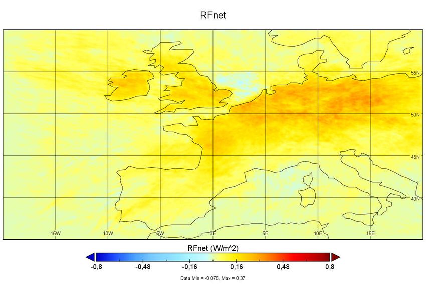
significantly larger than the 17 % decrease of CO2 emissions from global energy production in April 2020 compared
     to 2019 levels (Le Quéré et al., 2020).

65   This paper quantifies air traffic activity, the related contrail cirrus and the radiative forcing for Europe in the months
     March to August 2019 and 2020. A subsequent paper will compare the model results to satellite observations.A
     parallel paper compares the model results to satellite observations (Schumann et al., 2021). The investigation within
     20°W to 20°E and 35°N to 60°N covers much of Europe and the Eastern parts of the North Atlantic that have high
     air traffic density and are visible from the geostationary satellite METEOSAT (Schmetz et al., 2002).

70   The contrails are simulated with the Contrail Cirrus Prediction Model (CoCiP) (Schumann, 2012) which has been
     used for various related studies (Schumann et al., 2017; Voigt et al., 2017; Teoh et al., 2020b; Teoh et al., 2020a).
     The contrail model uses traffic data from EUROCONTROL for a large part of Europe and from the UK air
     navigation service provider NATS for the Shanwick Oceanic Control Area. Performance parameters, including fuel
     consumption and overall propulsion efficiency, are estimated using the Base of Aircraft Data (BADA 3) from
75   EUROCONTROL (Nuic et al., 2010; EUROCONTROL, 2015) and a recently developed open-access performance
     model for a set of subsonic turbofan-powered transport aircraft at cruise (Poll, 2018; Poll and Schumann, 2021b,
     a). Soot number emissions are computed with the fractal aggregate model (Teoh et al., 2019; Teoh et al., 2020b).
     The model uses numerical weather prediction forecast (FC) data from the European Centre for Medium Range
     Weather Forecasts (ECMWF) (Bauer et al., 2015). This paper describes the new traffic data set and its setup for
80   2019 and 2020. The data are used to quantify the changes in traffic, fuel consumption, soot emissions, contrail
     cover, RF and the related TOA irradiances. CoCiP is run in various model versions, to test the sensitivity of the
     results to model parameters, mainly in a new version approximating humidity exchange with background air and
     radiative contrail-contrail overlap, inspired by some earlier studies (Burkhardt and Kärcher, 2011; Schumann et al.,
     2015; Sanz-Morère et al., 2021). A set of parameter studies is presented that identify the model sensitivity to input
85   and model parameters. A further study of climatological effects and comparisons with satellite observation data,
     using simulations over a longer period is planned.

     2 Air traffic and aircraft emissions input

     This section briefly describes the data base of air traffic and aircraft emissions over Europe in 2019 and 2020 used
     for the contrail simulations. As a minimum, the input data must characterise the flights tracks and emissions in the
90   “upper” airspace above Flight Level (FL) 180 (18000 feet, about 5.5 km), where most contrails form. Previous
     CoCiP studies have used air traffic from various sources, including a global track data base for 2006 (Wilkerson et

                                                                 3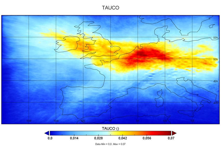
al., 2010; Brasseur et al., 2016), data collected for the field experiment ML-CIRRUS over Europe and the North
      Atlantic in March/April 2014 (Schumann et al., 2016; Voigt et al., 2017) or traffic data for six weeks distributed
      over one year in 2012/13 in Japanese airspace (Teoh et al., 2020b). Here, all flights passing the European
 95   investigation domain are considered. This includes all kerosene burning turbofan and turboprob engine aircraft.
      Piston engine powered aircraft only make a very small contribution to contrail formation. Input includes the aircraft
      type code, as defined by the International Civil Aviation Organization (ICAO), and the sequence of waypoints
      along the flight track. At each waypoint, the time, latitude, longitude, and FL, plus true air speed, instantaneous
      aircraft mass, fuel flow rate, overall propulsion efficiency and soot number emission index are specified, together
100   with a unique running flight number, and information on the traffic and the performance data sources used. The
      simulation code requires input in hourly sections with constant time resolution. The construction of this input starts
      with the list of flights inside or passing Europe, followed by the whole route from departure to the destination
      airport, which is required in order to estimate the aircraft take-off mass. This is then combined with meteorological
      wind and temperature data, and with performance and emission analyses, which is obtained from various sources
105   in a sequence of processing steps, see Supplement.

      The prime sources for the aircraft position information are the so-called Correlated Position Report (CPR) messages
      provided by EUROCONTROL’s Performance Review Unit (PRU). These data originate from the pan-European
      air traffic management system operated by EUROCONTROL (Niarchakou and Cech, 2019). The CPR represents
      augmented       surveillance     position     information,      based     on      real-time     surveillance     data
110   (https://www.eurocontrol.int/service/data-collection-service) derived from radar and from Automatic Dependent
      Surveillance - Broadcast (ADS-B) data (https://ads-b-europe.eu/). For flights outside the surveillance domain of
      EUROCONTROL, data from EUROCONTROL’s so-called Model 3 (M3) data (Wandelt and Sun, 2015) are used,
      which contain partial track information from departure to destination also outside Europe. The M3 data are flight
      plan data partly corrected by surveillance (radar) data and are available from the DDR2 data repository of
115   EUROCONTROL. The M3 files provided by the PRU come directly from the network manager archives. For
      flights in the Shanwick control zone of the North Atlantic flight corridor, track information was provided by NATS.
      These were used to either replace or augment M3 data in that zone. The CPR data come without the ICAO aircraft
      type codes, but about 70 % of the CPR data contain the so-called ICAO 24-bit code, which is a unique aircraft
      identifier. A table relating many of the 24-bit codes with aircraft types was made available to us by Martin Schäfer
120   within OpenSky (Schäfer et al., 2014). In other cases, the type code for CPR records was identified from the M3

                                                                4
or the NATS data for flights with same aircraft callsign, departure and destination locations and the same departure
time.
For comparisons (see Supplement), aircraft position data as collected from a distributed net of ground-received
ADS-B data and as purchased from Fligthradar24 AB, Sweden (https://www.flightradar24.com/how-it-works)
125 were used. In addition, checks were performed by comparisons of the trajectory position data to position data
obtained during flights of the DLR research aircraft. These confirmed that the position accuracy was inon the order
of 100 m in most cases.
Temperature and wind along the flight tracks are interpolated from global ERA5 reanalysis data, produced by
ECMWF within the Copernicus Climate Change Service (Hersbach et al., 2020). Here, global 3-houly data with 1-
130 degree geographic resolution, at pressure levels are used. True air speed is computed by subtracting the windspeed
vector from the groundspeed vector. Temperature is required for computing Mach and Reynolds numbers and
related aircraft performance parameters.
The contrail analysis requires information about the local aircraft mass, local fuel flow rate (in kg s-1) and overall
propulsion efficiency, together with water vapor mass and soot number emission indices per mass of burned fuel.
135 Sensitivity studies with CoCiP show that a 10 % change in fuel consumption causes a change of about 7 % in
contrail radiative forcing. Contrail formation depends on the overall propulsion efficiency, , and an increase in
of 0.1 increases the threshold temperature by about 1.5 K (Schumann, 2000). Hence, more contrails form for larger
. Since most aircraft travel at temperatures about 5 to 12 K below the threshold temperature (Schumann and
Heymsfield, 2017), the value of has a smaller impact on the total mean contrail properties.
140 The fuel consumption rates and the overall propulsion efficiency are obtained from an aircraft performance model.
In the past, the EUROCONTROL BADA3 model (Nuic et al., 2010; EUROCONTROL, 2015) was used for CoCiP
studies (Schumann et al., 2011a). Alternatively, and in view of known limitations of the BADA3 method (Nuic et
al., 2010), we use the self-contained and open source model “PS” presented recently (Poll and Schumann, 2021b,
a), with a slight modification to allow for the full range of Mach numbers at cruise. The PS method has a more
145 rigorous aerodynamic foundation and covers Reynolds number effects.
Fuel consumption rate is directly proportional to the aircraft mass, which is derived by subtracting the integrated
fuel mass burned from the take-off mass. The take-off mass is the sum of the operational empty aircraft mass, the
payload mass, and the total fuel mass. Unfortunately, take-off massmasses of aircraft isare not recorded in publicly
available data set. Consequently, the take-off mass is estimated using an assumed payload load factor, LF (ratio of
5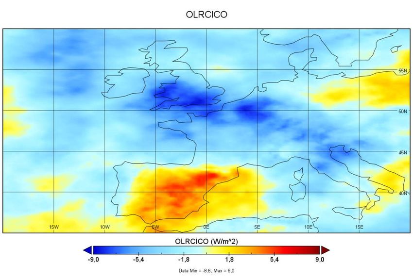
150 actual payload mass to maximum permitted payload mass). Data from the US Bureau of Transportation Statistics,
from the German Statistical Federal Office, from EUROCONTROL and from ICAO (see Supplement) suggest
lower passenger and freight loadings after March 2020 than in the previous year (and more cargo flights).
Therefore, LF is taken to be 0.7 for the time before the pandemic and 0.5 thereafter. The value 0.7 is found to be
consistent with the actually flown FL profile staying below BADA3’BADA3’s estimate of the maximum altitude
155 for the given mass (Eq. 3.5-1 (EUROCONTROL, 2015)) for most flights. The fuel mass is estimated from the total
flight distance in air and mean cruise aircraft performance. The overall propulsion efficiency, , is defined as the
product of engine net thrust and true air speed divided by the product of fuel flow rate and the lower calorific value
of fuel (Cumpsty and Heyes, 2015). Both the fuel flow rate and the net thrust are provided by the performance
model. The water vapor mass emission index and the lower calorific value of kerosene are set to 1.23 kg/kg and 43
160 MJ/kg, respectively.
Contrail properties are sensitive to the number of soot (or black carbon) particles emitted (Schumann et al., 2013a;
Kärcher, 2016; Burkhardt et al., 2018; Teoh et al., 2020b). For example, optical depth increases with the third root
of the soot number emission index (Schumann et al., 2013a). The soot number emission index depends strongly on
the engine type and operation state. Here, the emission index is computed for known engine types using engine
165 data from the ICAO emission data bank and recently developed methods (Teoh et al., 2019). The black carbon
(BC) number emissions index (EIn) is calculated using the Fractal Aggregates (FA) model (Teoh et al., 2020): it
estimates the BC EIn from the BC mass emissions index (BC EIm), particle size distribution (geometric mean
diameter, GMD, and its standard deviation, GSD) and morphology (Dfm): For each flight, the BC EIm is estimated
using the Formation and Oxidization Method (FOX) (Stettler et al., 2013) and Improved FOX method (ImFOX)
170 (Abrahamson et al., 2016), which are based on the thermodynamic and physical mechanisms by which BC is
formed and oxidized. More specifically, the FOX method requires the overall pressure ratio of each engine type as
an input to estimate the BC EIm, and we obtained this parameter from the ICAO Emission Data Bank (EDB). No
smoke number measurements are required in the FOX and ImFOX methods. Since recently, the ICAO EDB
provides non-volatile particle mass data; these are not used here because they are not available for older engines.
175 The formulas and constants used to calculate the remaining parameters (GMD, GSD and Dfm) can be found in Teoh
et al. (2020b). In the few cases when these data are not available, a constant soot number emission index of 1015
kg-1 is assumed. The mean emission index from this method is about 3×10¹⁵ kg-1, with large variability (Teoh et al.,
2020b). With this emission index, the number of ice crystals per fuel mass burned in young contrails would be
about a factor of two larger than observed (Schumann et al., 2013a). This may indicate a size or temperature
6
180   dependent efficiency of soot particles acting as cloud condensation and ice nucleus (Kärcher, 2016; Kleine et al.,
      2018; Lewellen, 2020). Therefore, the computed soot emission index value is halved in this study.

      All these data are configured flight by flight, from departure to destination, without temporal interpolation and,
      finally, the flight tracks above FL 180 are split hourly and interpolated uniformly with 60 s time resolution. The
      resulting CoCiP input files require 36.8 GB (Gigabytes) of disk storage for March-August 2019 and 10.6 GB for
185   the same period in 2020.

      The mean traffic flight distances with respect to air (from true air speed and time, not over ground) and mean fuel
      flow rates for the fleet of aircraft within the European investigation domain are listed in Table 3 for 2020 together
      with the percentage change relative to 2019. Figure 1 shows an example of the traffic tracks obtained from the
      various sources within two half-hour periods of 1 March 2020 (still “normal” traffic), one in the early morning with
190   strong traffic from North America over the North Atlantic and one later in the morning with high traffic density
      over Europe. It can be seen that the CPR tracks are in good agreement with those from Flightradar24 (FR24).
      Apparently, many aircraft were equipped with ADS-B receivers from which the FR24 data are derived. The NATS
      data extend the CPR tracks in the Shanwick zone over the North Atlantic and the M3 data extend traffic in regions
      where surveillance data are missing.

195   As a result of the sudden change in demand and permissions for air transport, fleet operations in 2020 were very
      different from 2019. As illustrated in Figure 2a, mean air traffic in upper airspace (above FL 180) over Europe
      decreased considerably after mid-March 2020. The total flight distance per day decreased by 72 % on average over
      the six-month period and by 91 % for the month of April in 2020 relative to 2019. Table 1 compares total air
      distance covered in flights above FL180 over the European domain in March-August 2020 compared to March-
200   August 2019. Here, aircraft are split into 5 mass classes, as explained in the table caption, depending on the
      maximum permitted take-off mass (MTOM), using BADA3 data for given ICAO aircraft types. In April 2020, the
      total distance flown decreased to 8.8 % of the April 2019 values. The reduction was strongest for light and medium
      sized aircraft, i.e. single aisle transport and business jets, whilst general aviation aircraft (< 20 Mg) and heavy
      aircraft, i.e. twin aisle transport and cargo, experienced smaller reductions. By July 2020, light aircraft flight
205   distances had returned to 70 % compared to the year before, whilst the average overall reduction was 23 %
      compared to July 2019.

      Figure 3 illustrates the spatial distribution of the mean traffic in terms of fuel consumption in the simulation domain
      for the six months on average in 2019 and 2020. Traffic and fuel consumption is largest along the route from

                                                                7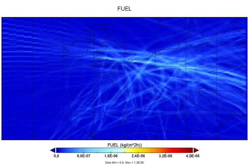
London, UK, to Frankfurt/Main, Germany, but spreads along many other routes from the North Atlantic to the Near
210   East and from Scandinavia to the Iberian Peninsula. Figure 3 also illustrates the large-scale traffic reduction in
      2020 compared to 2019. The decrease of fuel consumption and flight distances are similar because the relative
      increase in aircraft weight (more cargo aircraft) is largely balanced by the lower load factor.

      Table 1. Flight distances (in Gm) of general aviation/military jets (G: MTOM < 20 Mg), light (L: 20 < MTOM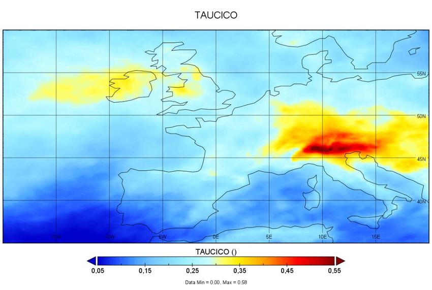
2019          7     50.29         0.018      0.008     50.31     99.9%         0.04% 0.016%          100%
                  2020          7     11.67         0.015      0.001     11.68     99.9%         0.12% 0.006%          100%
225

      3. Numerical weather prediction data

      Although 3-hourly ERA5 reanalysis pressure level data are used to provide the global traffic data with wind and
      temperature information, higher resolution deterministic operational numerical weather predictionsforecast (FC)
230   data from the Integrated Forecasting System (IFS) of the ECMWF (Bauer et al., 2015) are used for contrail
      simulation in the investigation domain. The IFS data are available for registered users. The IFS model used operates
      with a nominal resolution of 9 km horizontally, with 137 levels from the surface to model top at 0.01 hPa. Data are
      applied with 1 h time resolution and 0.25° horizontal geographic grid resolution. The mean vertical grid intervals
      in the IFS data between 200 and 300 hPa are about 10 hPa or 300 m for standard sea surface pressure. For
235   comparison, the ERA5 data used are provided at fixed pressure levels, including 300, 250, 225 and 200 hPa, with
      vertical height intervals varying between 670 and 1200 m, i.e., with a much coarser vertical resolution. The forecast
      (FC)forecasts provide hourly three-dimensional fields of pressure, temperature, wind components, humidity, ice
      water content and cloud cover, plus two-dimensional fields for TOA irradiances of incoming solar direct radiation
      (SDR), reflected solar (RSR) and outgoing longwave radiation (OLR) on average over the recent hour.

240   A critical issue in the simulation of persistent contrails is the relative humidity (RHi) with respect to saturation over
      ice (Schumann, 1996; Lamquin et al., 2012; Irvine and Shine, 2015; Schumann and Heymsfield, 2017; Gierens et
      al., 2020). Here, RHi is derived from the FC data for temperature, pressure and absolute humidity with given water
      vapor saturation pressure over ice (Sonntag, 1994). Several previous studies have found that ECMWF forecasts
      tend to underestimate the degree of ice supersaturation (Schumann and Graf, 2013; Kaufmann et al., 2018).

245   Figure 4 compares the probability density function of relative humidity derived from the IFS FC with data from
      ERA5 and the airborne in situ measurements on routine Airbus flights during the MOZAIC project (Petzold et al.,
      2020). Here, the FC and ERA5 data represent the RHi from interpolated temperature and absolute humidity along
      the flight tracks above Europe between 180 hPa and 310 hPa (about 12 and 8 km in the ICAO standard atmosphere)
      for the given time periods over Europe, while the MOZAIC data are from a longer time period and larger domain
250   at cruise levels of the Airbus A340, or A330 aircraft. Both NWP data sets underestimate the occurrence of high ice
      supersaturation. Part of this underestimate probably comes from the higher resolution of the measurements in time

                                                                 9
and space compared to the grid cell and hourly mean values provided by the numerical weather predictions. To
avoid an underestimate of simulated contrails, in the past, CoCiP simulations usually were performed with
enhanced humidity by dividing by a fixed model parameter RHic ≤ 1. Previously, in order to obtain reasonable
255 agreement between model estimates and the observations (Schumann and Graf, 2013) large changes have been
required (up to 1/RHic = 1/0.8 = 1.25). However, more recently the forecast resolution has improved and so an
RHic equal to 0.95 is used in the reference cases and 1.0 and 0.9 in parameter studies. The potential contrail cover,
i.e., the area fraction of air with temperature below the contrail threshold value and RHi > 100 % derived from the
FC data amounts to 15 % at FL 350 (10.6 km) on average over the investigation domain for RHic = 0.95, which
260 agrees with estimates in the literature (Gierens et al., 2012) and shows that the selected RHic value is reasonable.
While the results given in Figure 4 suggest that the quality of the ERA5 and FC data is about the same, the ERA5
data tend to underestimate wind shear, mainly because of the lower spatial resolution, see Figure 5. Wind shear is
important for simulating contrail dispersion. Without dispersion, contrails would remain narrow, triggering ice
clouds in the aircraft wake only (Lewellen, 2014; Paoli and Shariff, 2016). However, with shear and turbulence
265 driven dispersion, contrails grow in cross-section area and more and more contrail ice particles mix with ambient
air, converting ambient ice supersaturation into contrail ice particles.
Another important parameter is the vertical wind. Adiabatic upward motion conserves mass specific humidity, but
cools the air and, hence, enhances relative humidity, whilst downward motion reduces relative humidity (Gierens
et al., 2012). The thickness of ice supersaturated layers, with relative humidity between ice saturation and liquid
270 saturation in raising air masses, increases for decreasing ambient temperature (Gierens et al., 2012). Therefore,
vertical wind is controlling the persistence and lifetime of ice supersaturated air masses and contrails. Inspection
of several examples have shown that the ERA5 vertical wind is smoother in space and often smaller in magnitude
than in the FC. Consequently, the FC data are preferred for contrail simulations.
Figure 6 gives an indication of the vertical depth of those layers suited to the formation of persistent contrails - as
275 derived from the FC data. The air temperature inside these layers is below the Schmidt-Appleman threshold value
for contrail formation (for = 0.35) and humid enough for persistency (RHi>1) (Schumann, 1996). The computed
layer depth is limited by grid resolution and typically varies between 300 and 800 m, which is in the range of
observations (Gierens et al., 2012). The values are largest over mountains because of frequent upgliding motions.
Interestingly the thickness is larger over the North Atlantic than over the southern part of the domain. The geometric
280 thickness of layers with relative humidity between ice saturation and liquid saturation in raising air masses increases
for decreasing ambient temperature (Gierens et al., 2012) and the air temperature is lower at higher latitudes. Hence
10the thicker layers over the North Atlantic may be partly because of lower air temperature. The thickness of the ice
supersaturated layer limits the altitude range in which sedimenting ice particles persist and hence the thickness
influences maximum ice water content reached in contrails (Lewellen, 2014; Schumann et al., 2015).(Lewellen,
285 2014; Schumann et al., 2015). This ice water content and the geometrical depth also determine the optical thickness
and, hence, influence the radiative forcing from contrails. Finally, the ice supersaturated layer thickness is important
when discussing flight level changes to avoid warming contrails (Mannstein et al., 2005; Schumann et al., 2011a;
Teoh et al., 2020a). Figure 6 also shows that the mean layer thickness over most of Europe was significantly larger
in 2019 than in 2020, indicating that more contrails formed in 2019, not only because of more traffic, but also
290 because of more favourable contrail formation conditions.
4. Simulated contrail cover and related radiative forcing
The traffic, the emission input and the FC data described above are used for the contrail model CoCiP (Schumann,
2012). CoCiP simulates Lagrangian contrail segments from the initial formation in air satisfying the Schmidt-
Appleman criterion (Schumann, 1996) until the final decay for each 60-s flight segment. The contrail physics
295 represented in this model is partly simplified compared to other models (Lewellen, 2014; Paoli and Shariff, 2016;
Unterstrasser, 2016), but it resolves individual contrails and is applicable to global studies (Schumann et al., 2015).
The model computes the local, contrail induced RF of each contrail segment for given contrail properties and given
TOA solar and thermal irradiances using an algebraic model (Schumann et al., 2012) for an ice particle habit
mixture (see Table 2 in Schumann et al. (2011b)) fitted to a set of reference data from libRadtran (Mayer and
300 Kylling, 2005; Emde et al., 2016). The code reads the meteorological data hourly, so that only two time slices are
kept in the core storage at a given time. Contrails surviving the hour are kept in a separate buffer in core memory
and integrated in time over the next hour. The spatial distributions of contrail properties are evaluated each hour
on a grid with about a 4.2 km mean horizontal resolution prepared for comparisons with Meteosat-SEVIRI
observations (Schmetz et al., 2002) by summing the contributions from all the contrail segments, according to their
305 Gaussian plume properties. This gridded analysis consumes about 90 % of the computing time. Without this
evaluation part and after the preparation of all the input data, the Fortran code takes less than 5 min on a laptop
computer to run with traffic for the month of July 2019. The model parameters are set as described previously
(Schumann et al., 2015), but including variable soot number emission index EIs, humidity enhanced by a factor
1/RHic ( with RHic=0.95), plume mixing enhanced by differential radiative heating, contrail segments integrated
310 in the model’s Runge-Kutta scheme with 1800 s time steps, and 10 h maximum contrail life time.
11In regions of high traffic density, the amount of water entering contrails from ambient air may significantly
dehydrate ambient air (Burkhardt and Kärcher, 2011; Schumann et al., 2015). Contrails take up water vapor from
the ambient air and the first contrail formed reduces the ice supersaturation available for subsequent contrails flying
later along about the same track (Unterstrasser, 2020). As explained in Sanz-Morère et al. (2021), contrail-contrail
315 overlap also affects the radiative forcing. When one contrail is formed, it changes the irradiances OLR and RSR at
TOA. The RF is a function of these irradiances and reduced OLR and increased RSR values result in a smaller RF
from the next contrail. A complete modelling of the humidity exchange and overlap effects would require
integration of the prognostic equations for weather prediction and the related radiation transfer in time and space
with resolution corresponding to the contrail scales. This is beyond the state of the art. Here, we account for
320 humidity exchange with background air and contrail-contrail overlap in an approximate manner. For each contrail,
the mass of water vapor that enters as contrail ice is subtracted from the background field, and the mass of ice from
the sublimating contrails is returned to the background humidity, conserving total water mass in the corresponding
grid cell volume. To account for contrail-overlap in the RF analysis, the energy flux per grid cell area caused by
the LW RF from a contrail is subtracted from the TOA OLR so that the RF from a subsequent overlapping contrail
325 is driven by a reduced TOA flux. This ensures that the effective OLR (after subtraction of LW RF) stays positive.
For the SW flux, the albedo a=RSR/SDR is increased as a function of the SW RF, by RF SW/SDR. Here, SDR is
the (incoming) solar direct radiation. This ensures that the increased albedo stays below one. These corrections are
applied contrail by contrail in the sequence in which they occur in the traffic input and the changes in the
background air and TOA irradiances are lost when reading the next FC input hourly. The effects are demonstrated
330 in the next section.
The contrail model has been applied and tested in several previous studies (Voigt et al., 2010; Schumann et al.,
2011a; Jeßberger et al., 2013; Schumann and Graf, 2013; Schumann et al., 2013b; Schumann et al., 2013a;
Schumann et al., 2015; Schumann et al., 2017; Voigt et al., 2017; Teoh et al., 2020b). Figure 7 demonstrates that
the results from the improved method are both within the range of the previous results and within the scatter of
335 observation data for individual contrails. Without humidity exchange, the amounts of contrail ice, its particle sizes,
optical depth and geometrical width and depth are between 10 to 30 % larger. These changes are within the range
of scatter of the observations.
Figure 2 b-d show day-mean contrail properties and RF for the European domain as a function of time for the 6-
month period. The contrail contributions vary strongly from day to day because of variable weather. The ratio of
340 contrail distance to flight distance is similar in both years, with a slight tendency to smaller ratios in 2020 because
12of the drier air. Similarly, the LW and SW RF values vary strongly and partially in anti-correlation. Hence, the day
mean net RF is smaller, although positive on average. Some days with negative European mean net contrail RF are
also found.
Figure 8 gives the mean optical depth of the sum of all contrails from the simulations for six months in 2019 and
345 the difference 2019-2020 and Figure 9 shows the net RF. Both are computed taking humidity exchange with
background air and contrails overlap into account. TheThe given optical depth is the area mean of contrails per grid
cell. This optical depth is seen to reach values up to 0.07 on average over these six months, with maximum changes
of 0.054 between 2019 and 2020. However, it should be noted that this average includes contrail free days. Far
larger values are reached in individual contrail segments – see Figure 7. The mean area-coverage of contrails with
350 an optical depth larger than 0.1 decreased from 4.6 % in 2019 to 1.4 % in 2020. The mean cirrus cover in the
domain in these periods reaches up to 28 % (see Table 3). Hence, the computed relative changes in cirrus cover are
of the order of 10 % of mean cirrus cover.
The mean net RF varies from -0.2 to 0.8 W m-2 over Europe and is mostly positive. Mean negative values occur
over sea surfaces, mainly because of lower surface albedo than over land. Net RF values in 2020 are about 40 %
355 lower than those in 2019. Hence, the reduction in net RF (60 %) is smaller than the reduction in traffic (72 %). This
is due, in part, to different changes of SW and LW RF and to the nonlinear effects from contrail-background
humidity exchange and contrail-contrail overlap.
Finally, data are shown that may be compared withare comparable to satellite observations in a follow-on
study.(Vázquez-Navarro et al., 2013; Strandgren et al., 2017; Schumann et al., 2021). These are optical depth (OT),
360 OLR and RSR from the sum of cirrus and contrails. The OT presented in Figure 8 is sum of the OT of cirrus from
the FC data and the OT from contrails computed with CoCiP. Here, the OT of cirrus without contrails is estimated
from the weather model output as a function of ice water content and temperature with effective ice particle
diameters parameterized from observations at -81°C to 0°C temperatures (Heymsfield et al., 2014). The OLR given
in Figure 11 is from the FC data minus the LW RF from contrails and the RSR in Figure 12 is from the FC data
365 minus the SW RF from contrails. We see large spatial variability of cirrus OT and the irradiances. The variability
is largest for RSR because of changes in cloudiness, surface albedo, and seasonal changes in solar cycle. The plots
and the mean values (see Table 3) suggest that the year 2019 had more cirrus coverage with OT>0.1, less OLR and
less RSR compared to 2020. The differences show a band of changes between Ireland and the Balkan countries
which resemble the expected aviation effects but are overlaid by changes from different weather. A further
370 simulation with the weather of 2019 and traffic of 2020 quantifies the differences coming from the changes in
13weather. The mean contrail-cover in 2020, see Table 3, would have been 6 % larger if the weather in 2020 would
have been the same as in 2019. So, the weather impact on the contrail properties is smaller than the traffic impact
on contrails. Compared to the background atmosphere, the contrail induced changes reach about 10 % of the total
cirrus cover and the LW RF values reach an order 10 % of the spatial and temporal variability of OLR. The relative
375 contribution of SW RF to RSR is smaller because of larger variability of RSR.
Table 3: Mean air traffic and contrail properties for traffic and weather in various years
Case Unit 1 2 Ratio 3 Ratio
Traffic 2019 2020 cases 2020 cases
Weather 2019 2019 2/1 2020 3/1
Flight distance Mm d-1 21650 6110 28.2 % 6110 28.2 %
Fuel consumption Gg d-1 79.69 22.46 28.2 % 22.46 28.2 %
Flight level pressure altitude km 10.56 10.62 100.6 % 10.62 100.6 %
Flight level with contrails km 10.78 10.79 100.1 % 10.8 100.2 %
-1
Flight distance with contrails Mm d 1626 501.3 30.8 % 353.5 21.7 %
Contrail age h 2.029 2.073 102.2 % 2.118 104.4 %
Contrail optical thickness 1 0.088 0.100 114.0 % 0.104 118.5 %
Contrail particle volume mean radius µm 8.65 8.64 99.8 % 9.22 106.5 %
Contrail particle effective mean radius µm 14.4 14.5 100.4 % 15.3 106.3 %
Total cirrus coverage at OT > 0.1 1 0.278 0.264 94.9 % 0.249 89.5 %
Contrail coverage at OT > 0.1 1 0.0461 0.0149 32.4 % 0.0140 30.3 %
-2
IFS FC outgoing longwave radiation Wm 248.4 248.4 100.0 % 249.7 100.5 %
IFS FC reflected shortwave radiation W m-2 114.6 114.6 100.0 % 115 99.2 %
Longwave radiative contrail forcing W m-2 0.8992 0.285 31.7 % 0.2668 29.7 %
Shortwave radiative contrail forcing W m-2 -0.757 -0.215 28.4 % -0.2008 26.5 %
-2
Net radiative contrail forcing Wm 0.1422 0.07001 49.2 % 0.066 46.4 %
From plots like those shown in the lower panels of Figure 10 to Figure 12, one can read the maximum differences
380 between 2019-2020, as listed in Table 4. The extreme values in the differences 2019-2020 are positive for OT
and OLR and negative for RSR, as expected for larger contrail-cirrus cover in 2019 compared to 2020.
14Comparing the values in Table 4, we note that the changes in the mean differences 2019-2020 from total cirrus
and irradiances changes are 3 to 10 times larger than the changes to be expected in contrail cirrus OT and in LW
and SW RF components. Obviously, weather changes had a stronger effect on these satellite-observable
385 properties than air traffic in 2019/2020. In addition, we have to expect changes from other emissions (e.g., at the
surface) not modelled in this study.
Table 4: Extreme changes in contrail and total cirrus OT and irradiances between 2019 and 2020
2019-2020 2019-2020 Unit
Contrail OT 0.054 Total cirrus OT 0.15 1
LW RF 2.2 OLR - LW RF 8.6 W m-2
SW RF -2.1 RSR - SW RF -20 W m-2
5. Parameter Studies
390 In addition to the variations in weather and traffic, the results are sensitive to various model and input parameters.
5.1 Sensitivity to the performance model used
Results from BADA3 and the new PS method (Poll and Schumann, 2021b) are very similar for fuel consumption,
but there are large differences in the estimates of overall engine propulsion efficiency, . These have consequences
for the formation of contrails at threshold conditions. After preliminary studies showed that BADA3 overestimates
395 , we use BADA3 values reduced by factor 0.85 in the reference simulation in this paper. A total of 184 ICAO
aircraft types (or their BADA3-synonyms) contributed to the fuel consumption over Europe in 2019 (and similar
in 2020), 162 to contrails in the year 2019 and 154 in 2020. The PS model currently provides data for 54 of these
aircraft types. For traffic of 2019, the PS aircraft types account for 95 % of the fleet fuel consumption and 97 % of
the total contrail forcing. In 2020, their contribution to contrail forcing is 91 %. Hence, the PS model with aircraft
400 characteristics as given in the tables of Poll and Schumann (2021b) covers 91 to 97 % of relevant aircraft types.
Therefore, the PS method was used where possible and forPoll and Schumann (2021b) covers 91 to 97 % of relevant
aircraft types. Therefore, the PS method was used where possible. For aircraft types not covered in the current PS
method and for climb and descent phases, BADA3 data are used.
15As an aside, it was found that that 80 % (90 %) of fuel consumption over Europe comes from just 15 (23) aircraft
405 types, whilst 80 % (90 %) of the contrail forcing came from 13 (19) types in 2019 and from 16 (24) types in 2020.
In addition, 90 % of fuel consumption comes from 23 types, 90 % of contrail forcing comes from 19 types in 2019
and 24 in 2020. One particular aircraft type, a twin-engine medium-sized airliner, produced nearly 20 % of total
fuel consumption and 16 % of contrail forcing. In 2020,, in the same data set. The largest contrail contribution in
2020 came from one type of twin-engine heavy aircraft, probably as a result of the larger fraction of cargo flights
410 in 2020 (ICAO, 2021) (ICAO, 2021).
Table 3Table 5 compares results for one month’s traffic (July 2019) using the original BADA3 ( not corrected by
factor 0.85 as in the reference case) and PS. The integrated fuel consumption differs by less than 1 %. For individual
flights, the flight-mean fuel consumption values at FL above 180 exhibit a Pearson correlation coefficient of 0.998.
The mean values and standard deviations at cruise are 0.38±0.06 for BADA3 and 0.31±0.05 for PS with relative
415 mean difference of (20±9) % and mean correlation of 0.89. BADA3 tends to overestimate drag at cruise and, hence,
engine thrust, as confirmed by a few comparisons to alternative performance models (BADA4 (Nuic et al., 2010)
and PIANO (Simos, 2004)). Since contrails form at higher temperature for higher , more contrails form in the
model runs when BADA3 is used compared to when the PS model is used. As expected, the total contrail flight
distances differ by only about 3 % because many contrails occur at temperatures far below the threshold
420 temperature. The mean optical depth and the mean RF values are 3 to 5 % larger for BADA3 than for PS input.
Incidentally, the net RF changes with similar magnitude, but with a different sign because the added contrails for
higher occur mainly at lower altitudes contributing more to SW than to LW forcing. This clearly illustrates the
non-linearity of the climate impact of contrail formation.
425
Table 5: Sensitivity to the performance models
Parameter Unit BADA3 PS BADA3/PS Ratio
Flight distance Mm d-1 24210 24210 100.0 %
Fuel consumption Gg d-1 87.6 87.62 100.0 %
-1
Contrail distance Mm d 1552 1506 103.1 %
Mean age h 2.003 2.027 98.8 %
16Contrail optical thickness 1 0.1048 0.1003 104.5 %
Longwave RF W m-2 0.9583 0.933 102.7 %
Shortwave RF W m-2 -0.8359 -0.8075 103.5 %
Net RF W m-2 0.1225 0.1255 97.6 %
430 Table 6: Sensitivity to soot emission index in two CoCiP model versions
Model With exchange and overlap Without exchange or overlap
EIsoot/(1015 kg-1) 1.5 1 Ratio 1.5 1 Ratio
Fuel burned/Gg 87.6 87.6 100.0 % 87.6 87.6 100.0 %
Distance with contrails/Mm 1487 1493 99.6 % 1554 1554 100.0 %
Mean age/h 2.03 1.99 101.9 % 1.98 1.95 101.6 %
Mean optical thickness 0.102 0.083 122.9 % 0.118 0.094 125.5 %
Volume mean radius/µm 9.442 10.4 91.2 % 10.6 11.4 93.1 %
Effective radius/µm 15.18 16.5 92.2 % 17.6 18.7 94.2 %
Longwave RF/(W m-2) 0.9311 0.788 118.2 % 1.583 1.244 127.3 %
Shortwave RF/(W m-2) -0.8061 -0.655 123.0 % -1.221 -0.937 130.3 %
-2
Net RF/(W m ) 0.125 0.132 94.3 % 0.362 0.307 117.8 %
5.2 Sensitivity to soot emissions
The soot emission indices derived with the fractal aggregate model (Teoh et al., 2019) are, even after
multiplication with the above-mentioned adjustment factor 0.5, on average 50 % larger than the fixed value
1×10¹⁵ kg-1 used in an earlier CoCiP study (Schumann et al., 2015). As expected (Teoh et al., 2020b),
435
Table 6 shows that a 50 % larger soot emission index causes a slightly larger contrail age (2 %), larger optical
contrail thickness (25 %) and 20 to 30 % larger RF values, with largest impact on the SW part. The increased
particle number enhances SW effects more than LW. That is a known phenomenon, see figure 10 in Schumann et
al. (2012).
17440 5.3 Importance of relative humidity
Table 7: Sensitivity to mean ice supersaturation parameter RHic, absolute values and ratios relative to the
reference case 2.
Case 1 2 3 Ratios
RHic 1 0.95 0.9 1 to 2 3 to 2
Contrail distance/Mm 807.4 1487 2071 54 % 139 %
Mean age/h 2.04 2.03 2.05 100 % 101 %
Mean optical thickness 0.0867 0.102 0.124 85 % 122 %
Longwave RF 0.434 0.931 1.644 47 % 177 %
Shortwave RF -0.372 -0.806 -1.439 46 % 179 %
Net RF 0.061 0.125 0.205 49 % 164 %
The amount of ice supersaturation in the background atmosphere is the most important parameter for contrail
445 modelling. The inverse of the parameter RHic is used to enhance humidity. Table 7 shows the sensitivity of domain
mean values for one month with dense traffic (July 2019) to changes in RHic. Both absolute and relative values are
given, compared to the results for RHic = 0.95. As expected, both the contrail length (flight distance with contrail
formation) and their optical thickness increase strongly with increasing humidity. The overall impact of increasing,
or decreasing, RHic by 5 % are changes in net RF of order 60 %. Obviously, the sensitivity to RHic is significant
450 and the RHic value selected should be checked again when comparing the model results to observations.
Several other parameters are also important. For example, enhancing the vertical shear of horizontal wind by factor
of 2, or vertical diffusivities by similar amounts causes changes in RF of order 10 to 20 %.
5.4 Sensitivity to the water vapor exchange and contrail overlap model
As can be seen from Table 8, the water exchange reduces the contrail optical thickness and the RF values by 10 to
455 20 %, with the larger values being for the denser traffic in 2019. The water exchange causes less ice particle
sedimentation and, hence, increases contrail lifetime on average by 1 to 4 %, with the larger values for 2019 traffic.
This is consistent with the results from a study with CoCiP coupled to a climate model (Schumann et al., 2015).
Table 8: Effects of water exchange and contrail overlap
18Traffic 2019 2019 2019 2020 2020 2020
Water exchange no yes yes no yes yes
Overlap no no yes no no yes
Flight distance/Mm 24210 24210 24210 8202 8202 8202
Fuel mass burned/Gg 87.6 87.6 87.6 26.7 26.7 26.7
Contrail age/h 1.98 2.02 2.03 2.00 2.01 2.02
Optical thickness 0.12 0.10 0.10 0.12 0.11 0.11
Volume radius/µm 10.6 9.6 9.4 10.3 9.7 9.6
Effective radius/µm 17.6 15.4 15.2 17.0 15.6 15.5
Longwave RF/(W m-2) 1.583 1.280 0.931 0.429 0.384 0.329
Shortwave RF/(W m-2) -1.221 -0.993 -0.806 -0.322 -0.289 -0.260
Net RF/(W m-2) 0.362 0.288 0.125 0.107 0.095 0.070
Ratios of RF values
Longwave RF 100 % 81 % 59 % 100 % 89 % 77 %
Shortwave RF 100 % 81 % 66 % 100 % 90 % 81 %
Net RF 100 % 79 % 35 % 100 % 88 % 65 %
460 The contrail-contrail overlap causes a significant reduction in RF. In particular, the mean LW RF is reduced by 23
% for 2020 and by 41 % for 2019. The smaller reduction of the SW RF causes up to 65 % reduction in the net RF.
Hence, these overlap aspects are important when considering regions with high traffic density. The changes appear
to be larger than expected (Sanz-Morère et al., 2021). As predicted (Sanz-Morère et al., 2021), these overlap aspects
are important for regions with high traffic density.
465 6. Conclusions and Outlook
In connection with the COVID-19 pandemic, global air traffic was considerably less in 2020 with respect to 2019
levels. This study has quantified air traffic and contrail changes within a European dense traffic area (20°W-20°E,
35°N-60°N), from March to August 2020, compared to same months in 2019, using traffic data, emission estimates,
ECMWF weather ERA5 reanalysis and IFS forecast data and a contrail model. The traffic data show that total
470 flight-distance (in respect to air) in the European investigation domain for traffic operating above FL 180 was 72
% smaller in 2020 than in 2019. The changes in the total fuel consumption and soot emissions are similar. In the
19reference case, the model shows that the flight distance with persistent contrail formation was reduced even more
strongly, by 78 %, mainly because the weather conditions in 2020 were less favourable for contrail formation than
in 2019. The coverage of contrails with an optical depth larger than 0.1 decreased from 4.6 % in 2019 to 1.4 % in
475 2020. These are large changes in view of the about 25 to 28 % mean cirrus cover. The reduced contrail coverage
caused 70 % less LW and 73 % less SW RF with the consequential, and a significantly smaller reduction of 54 %
in net RF.
In order to cover flights contributing to contrail formation as completely as possible, traffic data have been derived
from a number of sources. There may still be gaps, or inaccuracies, over the Atlantic, where flight plan data have
480 been used. This is particularly true south of the Shanwick area and, possibly, further north and over Ireland, where
detailed traffic data are missing. In all other areas, the traffic should be accurately covered. The fuel consumption
is assessed using two performance models, BADA3 and the new PS, and the results are similar. In estimating fuel
use, the main uncertainty results from the unknown aircraft take-off mass. In this study, the take-off mass is
determined by using the aircraft characteristics and an assumed mass load factor, i.e. payload mass fraction of
485 maximum permitted payload. There are indications that the load factor was considerably reduced in the 2020
COVID-19 period. The new performance model PS provides a more accurate aircraft drag estimate at cruise giving
a 10 to 30 % reduction in the engine overall propulsion efficiency compared to BADA3. This affects contrails
under threshold conditions and reduces contrail cover by about 3 % in total. As shown recently (Teoh et al., 2020b),
the soot number emissions are larger than assumed in early contrail studies. A 50 % increase in the soot number
490 results in a 30 % higher net RF. This again shows the importance of soot emissions and related fuel properties
(Moore et al., 2017).
The contrail model includes a new, approximate method to account for water vapor exchange between contrails
and background air and for RF in case of contrail-contrail overlap. Water vapor exchange reduces the modelled RF
magnitudes by about 10 to 20 %, with larger values being for the denser traffic in 2019. The contrail-contrail
495 overlap has an even stronger effect because the irradiances depend on the area covered by contrails, while the
amount of water vapor exchange depends on the contrail volume and the volume fraction per grid cell of the rather
thin contrails is smaller than their area fraction. The 2020/2019 reductions in LW RF are larger than in SW RF
causing a smaller reduction in net RF.
It may not beThe 2020/2019 reductions in LW RF are larger than in SW RF and the net RF changed less than the
500 SW and LW parts in this study. The SW and LW RF values have opposing sign and their mean magnitudes are 4
to 6 times larger than the net RF. Hence, small changes in the RF components have large impact on the net RF.
20The SW and LW RF components are partially correlated. However, the correlation is far different from 100 %
because the SW and LW effects depend on different input values (temperature, solar zenith angle, system albedo,
incoming solar irradiance and outgoing longwave irradiance, etc.), and respond to changes in the input parameters
505 with different sensitivities. The SW/LW ratio also depends on the diurnal traffic cycle and the seasons considered.
Therefore, several reasons cause different relative changes of net RF compared to the LW and SW components.
The net RF may change more strongly than the LW and SW components in other situations.
It is not easy to identify air-traffic induced changes in cirrus and irradiances over Europe in observations. The
changes in total cirrus cover and irradiance values due to aviation are below 10 % of the background cirrus cover
510 and the TOA irradiances without air traffic, in particular for SW irradiances. The aviation induced changes are 3
to 10 times smaller than the mean differences in total cirrus and in TOA irradiances caused by weather changes in
2019-2020. These ratios are sensitive to model uncertainties. The 2019-2020 changes in weather may havehad
larger effects on contrail cirrus and its RF than the large traffic changes during COVID-19. Changes may also be
caused by other aircraft emission (e.g., nitrogen oxides) (Brasseur et al., 2016) and by surface emissions.
515 Still, the traffic changes are large and last longer than the six months investigated so far. The traffic and the
background atmosphere appear to be well characterized, and the contrail model has proven skill as demonstrated
here again by comparison to a set of contrail observations. Much of the weather impact on background cirrus and
irradiance changes 2019-2020 is described by the IFS weather model. A 10 % change in cirrus cover and 10 %
changes in OLR relative to the regional and temporal variability are not small, and regional and diurnal variation
520 patterns may be detectable in observations. This may allow for the detection of aviation-induced changes in that
region. It will be interesting to test this hypothesis.
Ideally one should have accurate and representative observations which allow to assess the accuracy of the model
predictions. However, when we started this study, such observations were not available. Even now, with some
recent observations (Schumann et al., 2021), the accuracy of model predictions can only be estimated because the
525 observations have their own limitations.
The COVID-19 pandemic provided a new and unique opportunity to study the impact of aviation on cloudiness
and radiative forcing. Further studies are needed to explain the differences between the model and observation
results because the observed changes are caused not only by contrails but also by other anthropogenic and natural
effects.
530
21Code and Data availability
The contrail model input and output data are available on requestKey input data and some of the output data, as far
as storage limits allowed, are and will be made accessible in a public data repository, see Supplement. Further
output and tThe contrail model code can be made available by the lead author on request.
535 Author contributions
US performed the study and wrote the manuscript.; IP contributed to performance modelling,; RT contributed to
contrail and soot modelling and preprocessed NATS data,; RK, ES, JM and GSK contributed traffic data and related
know how,; RB prepared the ECMWF data,; LB provided input for preparing comparisons to satellite data,; MS
and CV contributed to the conceptual design and many details of the study. All authors contributed to manuscript
540 editing.
Competing interests
The authors declare no competing interests.
22Figures
545
Figure 1: Geographic map of the European domain under consideration for contrail simulations with
coloured flight tracks for two half-hour example time periods of 1 March 2020, before the COVID-19 crisis.
Individual panels show track data from a) CPR (red), b) M3 (blue), c) FR24 (green) and d) from the
combination of CPR with M3 and NATS data for flights extending beyond the CPR range (black, blue, and
550 purple lines).
23Figure 2: Mean values of a) flight distance in air, b) ratio of mean flight distance with contrails to total flight
555 distance, c) longwave (LW) RF and d) net RF versus time from 1 March to 30 August in 2019 (black curves)
and 2020 (red). The data represent averages over the European domain and over a 24-h day.
24560 Figure 3: Mean fuel consumption (in kg m-2 h-1) over the European domain, March-August mean values,
2019 (top) and 2020 (bottom).
25565
Figure 4: Probability density of relative humidity over ice (RHi) from ECMWF IFS forecast data (FC, blue
lines) and ERA5 re-analysis data (green) along the traffic routes over Europe as in 2020, separately for
meteorology of 2019 and 2020. The dark red dashed curve represents the 1995-2010 MOZAIC data as in
figure 5a of Petzold et al. (2020).
26570
Figure 5: Probability density of vertical shear of horizontal wind normal to flight segments along the traffic
routes over Europe as in 2020, separately for FC and ERA5 meteorology as in Figure 4.
575
27You can also read


