ArrayTrack: A Fine-Grained Indoor Location System
←
→
Page content transcription
If your browser does not render page correctly, please read the page content below
ArrayTrack: A Fine-Grained Indoor Location System
                                              Jie Xiong and Kyle Jamieson
                                                   University College London

Abstract                                                             for example. Location-aware smartphone applications
With myriad augmented reality, social networking, and                on the horizon such as augmented reality-based build-
retail shopping applications all on the horizon for the              ing navigation, social networking, and retail shopping
mobile handheld, a fast and accurate location technology             demand both a high accuracy and a low response time.
will become key to a rich user experience. When roam-                A solution that offers a centimeter-accurate location ser-
ing outdoors, users can usually count on a clear GPS sig-            vice indoors would enable these and other exciting appli-
nal for accurate location, but indoors, GPS often fades,             cations in mobile and pervasive computing.
and so up until recently, mobiles have had to rely mainly               Using radio frequency (RF) for location has many
on rather coarse-grained signal strength readings. What              challenges. First, the many objects found indoors near
has changed this status quo is the recent trend of dramat-           access points (APs) and mobile clients reflect the en-
ically increasing numbers of antennas at the indoor ac-              ergy of the wireless signal in a phenomenon called mul-
cess point, mainly to bolster capacity and coverage with             tipath propagation. This forces an unfortunate tradeoff
multiple-input, multiple-output (MIMO) techniques. We                that most existing RF location-based systems make: ei-
thus observe an opportunity to revisit the important prob-           ther model this hard-to-predict pattern of multipath fad-
lem of localization with a fresh perspective. This paper             ing, or leverage expensive hardware that can sample the
presents the design and experimental evaluation of Ar-               wireless signal at a very high rate. Most existing RF
rayTrack, an indoor location system that uses MIMO-                  systems choose the former, building maps of multipath
based techniques to track wireless clients at a very fine             signal strength [2, 3, 34, 43], or estimating coarse differ-
granularity in real time, as they roam about a building.             ences using RF propagation models [11, 14], achieving
With a combination of FPGA and general purpose com-                  an average localization accuracy of between 60 cm [43]
puting, we have built a prototype of the ArrayTrack sys-             and meters: too coarse for the applications at hand.
tem. Our results show that the techniques we propose can                Systems based on ultrasound and RF sensors such
pinpoint 41 clients spread out over an indoor office envi-            as Active Badge [35], Bat [36], and Cricket [19] have
ronment to within 23 centimeters median accuracy, with               achieved accuracy to the level of centimeters, but usually
the system incurring just 100 milliseconds latency, mak-             require dedicated infrastructure to be installed in every
ing for the first time ubiquitous real-time, fine-grained              room in a building, an approach that is expensive, time
location available on the mobile handset.                            consuming, and requires maintenance effort.
                                                                        Recently, however, two new opportunities have arisen
1    Introduction                                                    in the design of indoor location systems:
The proliferation of mobile computing devices contin-                1. WiFi APs are incorporating ever-increasing numbers
ues, with handheld smartphones, tablets, and laptops                    of antennas to bolster capacity and coverage with
a part of our everyday lives. Outdoors, these devices                   multiple-input, multiple-output (MIMO) techniques.
largely enjoy a robust and relatively accurate location                 In fact, we expect that in the future, the number of
service from Global Positioning System (GPS) satellite                  antennas at the access point will increase several-
signals, but indoors where GPS signals don’t reach, pro-                fold, to meet the demand for MIMO links and spatial
viding an accurate location service is quite challenging.               multiplexing [1, 31], which increase overall capacity.
   Furthermore, the demand for accurate location infor-                 Indeed, the upcoming 802.11ac standard will spec-
mation is especially acute indoors. While the few meters                ify eight MIMO spatial streams, and 16-antenna APs
of accuracy GPS provides outdoors are more than suffi-                   have been available since 2010 [41].
cient for street-level navigation, small differences in lo-
cation have more importance to people and applications                    2. Meanwhile, WiFi AP density remains high: With our
indoors: a few meters of error in estimated location can                     experimental infrastructure excluded, transmissions
place someone in a different office within a building,                        from most locations in our testbed reach seven or
                                                                             more production network APs, with all but about five
                                                                             percent of locations reaching five or more such APs.
This material is based on work supported by the European Research Council
                                                                             Furthermore, by leveraging the signal processing that
under Grant No. 279976. Jie Xiong is supported by the Google European        is possible at the physical layer, an AP can extract in-
Doctoral Fellowship in Wireless Networking.                                  formation from a single packet at a lower SNR than

USENIX Association                10th USENIX Symposium on Networked Systems Design and Implementation (NSDI ’13) 71
what is required to receive and decode the packet.                      Antenna
                                                                            array
   This allows even more ArrayTrack APs to cooperate
   to localize clients than would be possible were the
   system to operate exclusively at higher layers.

ArrayTrack is an indoor localization system that exploits
the increasing number of antennas at commodity APs to                                         Packet detection (§2.1),
                                                                                                                          AntSel
                                                                                             diversity synthesis (§2.2)
provide fine-grained location for mobile devices in an in-
door setting. When a client transmits a frame on the air,                              8
multiple ArrayTrack APs overhear the transmission, and                                                             Access point
                                                                                      Circular buffer     1      (Hardware radio
each compute angle-of-arrival (AoA) information from
                                                                                                                       platform)
the clients’ incoming frame. Then, the system aggre-
gates the APs’ AoA data at a central backend server to                                       (Number of access points)
estimate the client’s location. While AoA techniques are                        ·Angle-of-arrival spectrum computation (§2.3)
already in wide use in radar and acoustics, the challenge                       ·Multipath processing algorithms (§2.4)
in realizing these techniques indoors is the presence of                        ·Maximum likelihood position estimation (§2.5)
strong multipath RF propagation in these environments.                                                      ArrayTrack server
To address this problem, we introduce novel system de-
                                                                   Figure 1: ArrayTrack’s high-level design for eight radio front-ends, di-
sign techniques and signal processing algorithms that re-          vided into functionality at each ArrayTrack access point and centralized
liably eliminate the effects of multipath, even in the rela-       server functionality. For clarity, we omit transmit path functionality of
tively common situations when little or no energy arrives          the access point.
on the direct path between client and AP.
   ArrayTrack advances the state of the art in localization        In the next section, we detail ArrayTrack’s design. An
in three distinct ways:                                            implementation discussion (§3) and performance evalu-
                                                                   ation (§4) then follow. We discuss related work in Sec-
1. To mitigate the effects of indoor multipath propaga-            tion 5, and Section 7 concludes.
   tion, ArrayTrack contributes a novel multipath sup-
   pression algorithm to effectively remove the reflec-             2     Design
   tion paths between clients and APs.                             We describe ArrayTrack’s design as information flows
2. Upon detecting a frame, an ArrayTrack AP quickly                through the system, from the physical antenna array,
   switches between sets of antennas, synthesizing new             through the AP hardware, and on to the central Array-
   AoA information from each. We term this technique               Track server, as summarized in Figure 1. First, Array-
   diversity synthesis, and find that it is especially useful       Track leverages techniques to detect packets at very low
   in the case of low AP density.                                  signal strength, so that many access points can overhear a
3. ArrayTrack’s system architecture centers around par-            single transmission (§2.1). Next, at each AP, ArrayTrack
   allel processing in hardware, at APs, and in software,          uses many antennas (§2.2) to generate an AoA spectrum:
   at the database backend, for fast location estimates.           an estimate of likelihood versus bearing (§2.3), and can-
                                                                   cels some of the effects of multipath propagation (§2.4).
   We implement ArrayTrack on the Rice WARP FPGA                   Finally, the system combines these estimates to estimate
platform and evaluate in a 41-node network deployed                location (§2.5), further eliminating multipath’s effects.
over one floor of a busy office space. Experimental re-
sults in this setting show that using just three APs, Array-       2.1    Packet detection and buffer management
Track can localize clients to a median 57 cm and mean              To compute an AoA spectrum for a client, the AP only
one meter accuracy. With six APs, ArrayTrack achieves              need overhear a small number of frames (between one
a median 23 cm and mean 31 cm location accuracy, lo-               and three, for reasons that will become clear in Sec-
calizing 95% of clients to within 90 cm. At the same               tion 2.4) from that client. For ArrayTrack’s purposes, the
time, ArrayTrack is fast, requiring just 100 milliseconds          contents of the frame are immaterial, so our system can
to produce a location estimate. To our knowledge, these            process control frames such as acknowledgments, and
are the most accurate and responsive location estimates            even frames encrypted at the link layer.
available to date for an RF-based location system that                The physical-layer preamble of an 801.11 frame con-
does not require infrastructure except a normal density            tains known short and long training symbols, as shown in
of nearby WiFi APs. Furthermore, as we experimen-                  Figure 2. We use a modified version of Schmidl-Cox [25]
tally show, ArrayTrack’s performance is robust against             detection to detect an incoming frame’s short training
different antenna heights, different antenna orientation,          symbols. Once the detection block senses a frame, it
low SNR and collisions.                                            activates the diversity synthesis mechanism described in

                                                               2
72 10th USENIX Symposium on Networked Systems Design and Implementation (NSDI ’13)                                 USENIX Association
800 ns 3.2 μs 3.2 μs
s 0 s1 s2 s 3 s 4 s 5 s 6 s 7 s 8 s 9 G S0 S1
Figure 2: The 802.11 OFDM preamble consists of ten identical, re- 0 -0.3 -0.6 -0.3 0
peated short training symbols (denoted s0 . . . s9 ), followed by a guard Relative power (dB)
interval (denoted G), ending with two identical, repeated long training
symbols (denoted S0 and S1 ). Figure 3: The AoA spectrum of a client’s received signal at a multi-
antenna access point estimates the incoming signal’s power as a func-
tion of its angle of arrival.
the next section and stores the samples of the incoming
frame into a circular buffer, one logical buffer entry per nel, and so we can treat the information obtained from
frame detected. each set of antennas as if the two sets were obtained si-
Since it does not require even a partial packet decode, multaneously from different radios at the AP.
our system can process any part of the packet, which is
helpful in the event of collisions in a carrier-sense mul-
2.3 AoA spectrum generation
tiple access network (§4.3.5). Our system detects the
preamble of the packet and records a small part of it. In Especially in indoor wireless channels, RF signals re-
principle, one time domain packet sample would provide flect off objects in the environment, resulting in mul-
enough information for the AoA spectrum computation tiple copies of the signal arriving at the access point:
described in Section 2.3. However, to average out the ef- this phenomenon is known as multipath propagation. An
fects of noise, we use 10 samples (we justify this choice AoA spectrum of a client’s received signal at a multi-
in Section 4.3.3). Since a commodity WiFi AP samples antenna AP is an estimate of the incoming signal’s power
at 40 Msamples/second, this implies that we need to pro- as a function of angle of arrival, as shown in Figure 3.
cess just 250 nanoseconds of a packet’s samples, under Since strong multipath propagation is present indoors,
1.5% of an WiFi preamble’s 16 μs duration. the direct-path signal may be significantly weaker than
the reflected-path signals, or may even be undetectable.
2.2 Diversity synthesis In these situations, the highest peak on the AoA spec-
Upon detecting a packet, most commodity APs switch trum would correspond to a reflected path instead of the
between pairs of antennas selecting the antenna from direct path to the client. This makes indoor localization
each pair with the strongest signal, a technique called using AoA spectra alone highly inaccurate, necessitating
diversity selection. This well-known and widely imple- the remaining steps in ArrayTrack’s processing chain.
mented technique improves performance in the presence
of destructive multipath fading at one of the antennas, 2.3.1 Phased-array primer
and can be found in the newest 802.11n MIMO access In order to explain how we generate AoA spectra, we
points today. It also has the advantage of not increasing now present a brief primer on phased arrays. While their
the number of radios required, thus saving cost at the AP. technology is well established, we focus on indoor appli-
ArrayTrack seamlessly incorporates diversity selec- cations, highlighting the resulting complexities.
tion into its design, synthesizing independent AoA data For clarity of exposition, we first describe how an AP
from both antennas of the diversity pair. We term this can compute angle of arrival information in free space
technique diversity synthesis. (i.e., in the absence of multipath reflections), and then
Referring to Figure 1, once the packet detection block generalize the principles to handle multipath wireless
has indicated the start of a packet, control logic stores propagation. The key to computing a wireless signal’s
the samples corresponding to the preamble’s long train- angle of arrival is to analyze received phase at the AP,
ing symbol S0 (Figure 2) from the upper set of antennas a quantity that progresses linearly from zero to 2π ev-
into the first half of a circular buffer entry. Next, the con- ery RF wavelength λ along the path from client to access
trol logic toggles the AntSel (for antenna select) line in point, as shown in Figure 4 (left).
Figure 1, switching to the lower set of antennas for the This means that when the client sends a signal, the AP
duration of the second long training symbol S1 .1 Since S1 receives it with a phase determined by the path length d
and S2 are identical and each 3.2 μs long, they fall well from the client. Phase is particularly easy to measure at
within the coherence time2 of the indoor wireless chan- the physical layer, because software-defined and hard-
1 We use the long training symbols because our hardware radio plat- ware radios represent the phase of the wireless signal
form has a 500 ns switching time during which the received signal is graphically using an in-phase-quadrature (I-Q) plot, as
highly distorted and unusable.
2 The time span over which the channel can be considered stationary. shown in Figure 4 (right), where angle measured from
Coherence time is mainly a function of the RF carrier frequency and the I axis indicates phase. Using the I-Q plot, we see that
speed of motion of the transmitter, receiver, and any nearby objects. a distance d adds a phase of 2πd/λ as shown by the angle
3
USENIX Association 10th USENIX Symposium on Networked Systems Design and Implementation (NSDI ’13) 73Signal e-vector e2
Access point 1 λ/2 2
x1 Q
2πd/λ x3
d θ π sin θ Signal subspace
θ
½λ sin θ I
λ x2 a(θ) continuum
a(θ2)
Client
Figure 4: Principle of operation for ArrayTrack’s AoA spectrum com- a(θ1)
putation phase. (Left:) The phase of the signal goes through a 2π x2
cycle every radio wavelength λ, and the distance differential between Signal Noise
the client and successive antennas on the access point is related to the e-vector e1 e-vector e3
client’s bearing on the access point. (Right:) The complex representa- x1
tion of the sent signal at the client (filled dot) and received signals at
Figure 5: In this three-antenna example, the two incoming signals
the access point (crosses) reflects this relationship.
(at bearings θ1 and θ2 respectively) lie in a three-dimensional space.
Eigenvector analysis identifies the two-dimensional signal subspace
shown, and MUSIC traces along the array steering vector continuum
measured from the I axis to the cross labeled x1 (repre- measuring the distance to the signal subspace. Figure adapted from
senting the signal received at antenna one). Since there is Schmidt [26].
a λ/2 separation between the two antennas, the distance
along a path arriving at bearing θ is a fraction of a wave- So we can express what the AP hears as
length greater to the second antenna than it is to the first, ⎡ ⎤
that fraction depending on θ. Assuming d � λ/2, the A
s1 (t)
� �� �⎢ ⎥
⎢ s2 (t) ⎥
added distance is 12 λ sin θ.
x(t) = [a(θ1 ) a(θ2 ) · · · a(θD )] ⎢ . ⎥ + n(k), (3)
⎣ .. ⎦
These facts suggest a particularly simple way to com-
pute θ at a two-antenna access point in the absence of sD (t)
multipath: measure x1 and x2 directly, compute the phase
of each (∠x1 and ∠x2 ), then solve for θ as where n(k) is noise with zero mean and σn2 variance. This
means that we can express Rxx as
� �
∠x2 − ∠x1 Rxx = E[xx∗ ]
θ = arcsin (1)
π = E [(As + n) (s∗ A∗ + n∗ )]
= AE [ss∗ ] A∗ + E [nn∗ ]
Generalizing to multiple antennas. In indoor multi- = ARss A∗ + σn2 I (4)
path environments, Equation 1 quickly breaks down, be-
cause multiple paths’ signals sum in the I-Q plot. How- where Rss = E [ss∗ ] is the source correlation matrix.
ever, adding multiple, say M, antennas can help. The best The array correlation matrix Rxx has M eigenvalues
known algorithms are based on eigenstructure analysis of λ1 , . . . , λM associated respectively with M eigenvectors
an M×M correlation matrix Rxx in which the entry at the E = [e1 e2 · · · eM ]. If the noise is weaker than the in-
lth column and mth row is the mean correlation between coming signals, then when the eigenvalues are sorted in
the lth and mth antennas’ signals. non-decreasing order, the smallest M − D correspond to
Suppose D signals s1 (t), . . . , sD (t) arrive from bear- the noise while the next D correspond to the D incoming
ings θ1 , . . . , θD at M > D antennas, and that xj (t) is the signals. The D value depends on how many eigenvalues
received signal at jth antenna element at time t. Recall- are considered big enough to be signals. We choose D
ing the relationship between measured phase differences value as how many eigenvalues are larger than a thresh-
and AP bearing discussed above, we use the array steer- old that is a fraction of the largest eigenvalue. Based on
ing vector a(θ) to characterize how much added phase this process, the corresponding eigenvectors in E can be
(relative to the first antenna) we see at each of the other classified as noise or signal:
antennas, as a function of the incoming signal’s bearing. ⎡ ⎤
For a linear array, EN ES
� �� � � �� �
E = ⎣e1 . . . eM−D eM−D+1 . . . eM ⎦ (5)
⎡ ⎤
1
� �⎢
⎢ exp(−jπλ cos θ) ⎥
⎥ we refer to EN as the noise subspace and ES as the signal
−j2πd ⎢ exp (−j2πλ cos θ) ⎥
a(θ) = exp ⎢ ⎥ (2) subspace.
λ ⎢ .. ⎥
⎣ . ⎦ The MUSIC AoA spectrum [26] inverts the distance
exp (−j(M − 1)πλ cos θ) between a point moving along the array steering vector
4
74 10th USENIX Symposium on Networked Systems Design and Implementation (NSDI ’13) USENIX AssociationScenario Frequency
Direct path same; reflection paths changed 71%
x1 x2 x3 x4 x5 x6 x7 x8 Direct path same; reflection paths same 18%
Direct path changed; reflection paths changed 8%
Figure 6: Spatial smoothing an eight-antenna array x1 , . . . , x8 to a vir- Direct path changed; reflection paths same 3%
tual six-element array (number of groups NG = 3).
Table 1: Peak stability microbenchmark measuring the frequency of
NO spatial smoothing (SS) SS with 2 sub−array groups the direct and reflection-path peaks changing due to slight movement.
90 90
60 1 120 60 1 120
30 0.5
150 30 0.5
150
2.3.3 Array geometry weighting
Information from the linear array we use in our sys-
0 180 0 180 tem is not equally reliable as a function of θ, because
of the asymmetric physical geometry of the array. Con-
SS with 3 sub−array groups SS with 4 sub−array groups
90 90
sequently, after computing a spatially-smoothed MUSIC
60 120 60 120 AoA spectrum, the ArrayTrack multiplies it by a win-
270 270
30 0.5 150 30 0.5 150 dowing function W(θ), the purpose of which is to weight
information from the AoA spectrum in proportion to the
0 180 0 180 confidence that we have in the data. With a linear array,
Figure 7: Varying the amount of spatial smoothing on AoA spectra. we multiply P(θ) by
continuum and ES , as shown in Figure 5: 1, if 15◦ < |θ| < 165◦
W (θ) = (7)
sin θ, otherwise.
1
P(θ) = (6)
a(θ)EN E∗N a(θ) 2.3.4 Array symmetry removal
Although a linear antenna array can determine bearing,
This yields sharp peaks in P(θ) at the signals’ AoA. it cannot determine which side of the array the signal is
arriving from. This means that the AoA spectrum is es-
sentially a 180◦ spectrum mirrored to 360◦ . When there
2.3.2 Spatial smoothing for multipath distortion
are many APs cooperating to determine location, this is
Implementing MUSIC as-is, however, yields highly dis- not a problem, but when there are few APs, accuracy suf-
torted AoA spectra, for the following reason. When the fers. To address this, we employ the diversity synthesis
incoming signals are phase-synchronized with each other scheme described in Section 2.2 to have a ninth antenna
(as results from multipath) MUSIC perceives the distinct not in the same row as the other eight included. Using
incoming signals as one superposed signal, resulting in the ninth antenna, we calculate the total power on each
false peaks in P(θ). We therefore adopt spatial smooth- side, and remove the half with less power, resulting in a
ing [28], averaging incoming signals across NG groups of true 360◦ AoA spectrum.
antennas to reduce this correlation. For example, spatial
smoothing over NG = 3 six-antenna groups on an eight- 2.4 Multipath suppression
antenna array generating signals x1 , . . . , x8 would output While the spatial smoothing algorithms described above
six signals ẋ1 , . . . , ẋ6 where ẋi = 13 (xi + xi+1 + xi+2 ) for (§2.3.2) reduce multipath-induced distortion of the AoA
1 ≤ i ≤ 6, as shown in Figure 6. spectrum to yield an accurate spectrum, they don’t iden-
How should we choose NG ? Figure 7 shows a mi- tify the direct path, leaving multipath reflections free to
crobenchmark computing MUSIC AoA spectra for a reduce system accuracy. The multipath suppression al-
client near and in the line of sight of the AP (so the direct- gorithm we present here has the goal of removing or re-
path bearing dominates P(θ)) both with and without spa- ducing peaks in the AoA spectrum not associated with
tial smoothing. As NG increases, the effective number of the direct path from AP to client.
antennas decreases, and so spatial smoothing can elimi- ArrayTrack’s multipath suppression algorithm lever-
nate smaller peaks that may correspond to the direct path. ages changes in the wireless channel that occur when the
On the other hand, as NG increases, the overall noise in transmitter or objections in the vicinity move by group-
the AoA spectrum decreases, and some peaks may be ing together AoA spectra from multiple frames, if avail-
narrowed, possibly increasing accuracy. Based on this able. Our method is motivated by the following observa-
microbenchmark and experience generating AoA spectra tion: when there are small movements of the transmitter,
indoors from a number of different clients in our testbed, the receiver, or objects between the two, the direct-path
we find that a good compromise is to set NG = 2, and we peak on the AoA spectrum is usually stable while the
use this in the performance evaluation in Section 4. reflection-path peaks usually change significantly, and
5
USENIX Association 10th USENIX Symposium on Networked Systems Design and Implementation (NSDI ’13) 75Algorithm (Multipath suppression)
1. Group two to three AoA spectra from frames spaced
closer than 100 ms in time; if no such grouping ex- x AP 1 θ1
ists for a spectrum, then output that spectrum to the
synthesis step (§2.5). AP 2
2. Arbitrarily choose one AoA spectrum as the primary, θ2
and remove peaks from the primary not paired with Figure 10: ArrayTrack combines information from multiple APs into
peaks on other AoA spectra. a likelihood of the client being at location x by considering all AoA
3. Output the primary to the synthesis step (§2.5). spectra at their respective bearings (θ1 , θ2 ) to x.
Figure 8: ArrayTrack’s multipath suppression algorithm.
Primary
Figure 11: Left: the ArrayTrack prototype AP is composed of two
WARP radios, while a cable-connected USRP2 software-defined radio
-1 -0.5 0 0.5 1 0 -0.3 -0.6 -0.3 0 (not shown) calibrates the array. Right: The AP mounted on a cart,
showing its antenna array.
Figure 9: ArrayTrack’s multipath suppression algorithm operating on
two example AoA spectra (left) and the output AoA spectrum (right).
likelihood of the client being at location x, L(x), as
these slight movements happen frequently in real life N
when we hold a mobile handset making calls, for exam- L(x) = Pi (θi ) . (8)
ple. i=1
We run a microbenchmark at 100 randomly chosen lo-
cations in our testbed (see Figure 12, p. 7), generating With Equation 8 we search for the most likely location
AoA spectra at each position selected and another posi- of the client by forming a 10 centimeter by 10 centimeter
tion five centimeters away. If the corresponding bearing grid, and evaluating L(x) at each point in the grid. We
peaks of the two spectra are within five degrees, we mark then use hill climbing on the three positions with highest
that bearing as unchanged. If the variation is more than L(x) in the grid using the gradient defined by Equation 8
five degrees or the peak vanishes, we mark it changed. to refine our location estimate.
The results are shown in Table 1. Most of the time,
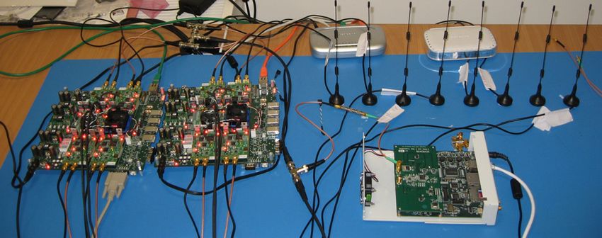
3 Implementation
the direct-path peak is unchanged while the reflection-
path peaks are changed. This motivates the algorithm The prototype ArrayTrack AP, shown in Figure 11, uses
shown in Figure 8. Note that for those scenarios in two Rice WARP FPGA-based wireless radios. Each
which both the direct-path and reflection-path peaks are WARP is equipped with four radio front ends and four
unchanged, we keep all of them without any deleterious omnidirectional antennas. We utilize the digital I/O pins
consequences. Also, observe that the microbenchmark on one of the WARP boards to output a time synchroniza-
above only captures two packets. This leaves room for tion pulse on a wire connected between the two WARPs,
even further improvement if we capture multiple packets so that the second WARP board can record and buffer the
during the course of the mobile’s movement. The only same time-indexed samples as the first. The WARPs run
scenario which induces failure in the multipath suppres- a custom FPGA hardware design architected with Xilinx
sion algorithm is when the reflection-path peaks remain System Generator for DSP that implements all the func-
unchanged while the direct-path peak is changed. How- tionality described in Section 2.
ever, as shown above, the chances of this happening are We place the 16 antennas3 attached to the WARP ra-
small. We show and example of the algorithm’s opera- dios in a rectangular geometry (Figure 11, right). Anten-
tion in Figure 9. nas are spaced at a half wavelength distance (6.13 cm) to
yield maximum AoA spectrum resolution. This also hap-
2.5 AoA spectra synthesis pens to yield maximum MIMO wireless capacity, and so
is the arrangement preferred in commodity APs.
In this step, ArrayTrack combines the AoA spectra of
several APs into a final location estimate. Suppose AP phase calibration. Equipping the AP with multi-
N APs generate AoA spectra P1 (θ), . . . , PN (θ) as pro- ple antennas is necessary for ArrayTrack, but does not
cessed by the previous steps, and we wish to compute 3 Thetwo WAPPs have a total of eight radio boards, each with two
the likelihood of the client being located at position x
ports. ArrayTrack is able to switch ports as described in §2.2 and record
as shown in Figure 3. ArrayTrack computes the bearing the two long training symbols with different antennas. So with two
of x to AP i, θi , by trigonometry, and then estimates the WARPs, the maximum number of antennas we can utilize is 16.
6
76 10th USENIX Symposium on Networked Systems Design and Implementation (NSDI ’13) USENIX Associationsuffice to calculate angle of arrival as described in the
preceding section. Each radio receiver incorporates a
2.4 GHz oscillator whose purpose is to convert the in-
6
coming radio frequency signal to its representation in I-Q 1
space shown, for example, in Figure 4 (p. 4). An unde- 4
sirable consequence of this downconversion step is that it 3 2
introduces an unknown phase offset to the resulting sig-
nal, rendering AoA inoperable. This is permissible for 5
MIMO, but not for our application, because this man-
ifests as an unknown phase added to the constellation
points in Figure 4. Our solution is to calibrate the array
with a USRP2 generating a continuous wave tone, mea-
Figure 12: Testbed environment: Soekris clients are marked as small
suring each phase offset directly. Because small man-
dots, and the AP locations are labelled “1”–“6”.
ufacturing imperfections exist for SMA splitters and ca-
bles labelled the same length, we propose a one-time (run
Experimental methodology. We place prototype APs
only once for a particular set of hardware) calibration
at the locations marked “1”–“6” in our testbed floorplan,
scheme to handle these equipment imperfections.
shown in Figure 12. The layout shows the basic struc-
The signal from the USRP2 goes through splitters and
ture of the office but does not include the numerous cu-
cables (we called them external paths) before reaching
bicle walls also present. We place the 41 clients roughly
WARP radios. The phase offset Phoff we want to
uniformly over the floorplan, covering areas both near
measure is the internal phase difference Phin2 − Phin1 .
to, and far away from the AP. We put some clients near
Running calibration once, we obtain the following offset:
metal, wood, glass and plastic walls to make our experi-
ments more comprehensive. We also place some clients
Phoff 1 = (Phex2 + Phin2 ) − (Phex1 + Phin1 ) (9)
behind concrete pillars in our office so that the direct path
Because of equipment imperfections, Phex2 is slightly between the AP and client is blocked, making the situa-
different from Phex1 so Phoff 1 is not equal to Phoff . We tion more challenging.
exchange the external paths and run calibration again: To measure ground truth in the location experiments
Phoff 2 = (Phex1 + Phin2 ) − (Phex2 + Phin1 ) (10) presented in this section, we used scaled architectural
drawings of our building combined with measurements
Combing the above two equations, we obtain Phoff and taken from a Fluke 416D laser distance measurement de-
the phase difference caused by equipment imperfections: vice, which has an accuracy of 1.5 mm over 60 m.
(Phoff 2 + Phoff 1 )/2 = Phoff (11) Due to budget constraints, we used one WARP AP,
moving it between the different locations marked on the
(Phoff 2 − Phoff 1 )/2 = Phex1 − Phex2 (12) map in Figure 12 and receiving new packets to emulate
Subtracting the measured phase offsets from the in- many APs receiving a transmission simultaneously. This
coming signals over the air then cancels the unknown setup does not favor our evaluation of ArrayTrack.
phase difference, and AoA becomes possible.
4.1 Static localization accuracy
Testbed clients. The clients we use in our experiments
are Soekris boxes equipped with Atheros 802.11g radios We first evaluate how accurately AoA pseudospectrum
operating in the 2.4 GHz band. computation without array geometry weighting and re-
flection path removing localizes clients. This represents
4 Evaluation the performance ArrayTrack would obtain in a static en-
To show how well ArrayTrack performs in real indoor vironment without any client movement, or movement
environment, we present experimental results from the nearby. The curves labeled three APs, four APs, five
testbed described in Section 3. First we present the accu- APs, and six APs in Figure 13 show raw location error
racy level ArrayTrack achieves in the challenging indoor computed with Equation 8 across all different AP com-
office environment and explore the effects of number of binations and all 41 clients. We see that the general trend
antennas and number of APs on the performance of Ar- is that average error decreases with an increasing number
rayTrack. After that, we demonstrate that ArrayTrack is of APs. The median error varies from 75 cm for three
robust against different transmitter/receiver heights and APs to 26 cm for six APs. The average error varies from
different antenna orientations between clients and APs. 317 cm for three APs to 38 cm for six APs. We show a
Finally we examine the latency introduced by Array- heatmap combination example in Figure 14 with increas-
Track, which is a critical factor for a real-time system. ing number of APs.
7
USENIX Association 10th USENIX Symposium on Networked Systems Design and Implementation (NSDI ’13) 77One AP Two APs Three APs Four APs Five APs Six APs
Figure 14: Heatmaps showing the location likelihood of a client with differing numbers of APs computing its location. We denote the ground truth
location of the client in each by a small dot in each heatmap.
1
1 6 APs (without optimization) ArrayTrack for 6 APs
5 APs (without optimization) 0.5
6 APs (unoptimized)
0.9
4 APs (without optimization)
0.8 3 APs (without optimization) 0 −1 0 1 2 3
10 10 10 10 10
0.7 1
ArrayTrack for 5 APs
0.6
5 APs (unoptimized)
CDF
0.5
0.5
0 −1
0.4 10 10
0 1
10 10
2 3
10
0.3 1
ArrayTrack for 4 APs
0.2 4 APs (unoptimized)
0.5
0.1
0 −1 0 1 2 3
10 10 10 10 10
0
1 5 10 20 50 100 500 2500
1
Location error (cm) ArrayTrack for 3 APs
3 APs (unoptimized)
Figure 13: Cumulative distribution of location error from unoptimized 0.5
raw AoA spectra data across clients using measurements taken at all
combinations of three, four, five, and six APs. 0 −1 0 1 2 3
10 10 10 10 10
Location error (cm)
4.2 Semi-static localization accuracy
Figure 15: Cumulative distribution of location error across clients for
We now evaluate ArrayTrack using data that incorpo- three, four, five and six APs with ArrayTrack.
rates small (less than 5 cm) movements of the clients,
with two more such location samples per client. This is tion performance. In these cases, we enable the array
representative of human movement even when station- symmetry removal scheme described in Section 2.3.4 to
ary, due to small inadvertent movements, and covers all significantly enhance accuracy. By using this technique,
cases where there is even more movement up to walking ArrayTrack can achieve a median 57 cm accuracy lev-
speed. In Figure 15, we show that ArrayTrack improves els with only three APs, good enough for many indoor
the accuracy level greatly, especially when the number applications.
of APs is small. Our system improves mean accuracy
level from 38 cm to 31 cm for six APs (a 20% improve- 4.2.1 Varying number of AP antennas
ment). We measure 90%, 95% and 98% of clients to be We now show how ArrayTrack performs with differing
within 80 cm, 90 cm and 102 cm respectively of their number of antennas at APs. In general, with more an-
actual positions. This improvement is mainly due to the tennas at each AP, we can achieve a more accurate AoA
array geometry weighting, which removes the relatively spectrum and capture a higher number of reflection-path
inaccurate parts of the spectrum approaching 0 degrees bearings, which accordingly increases localization ac-
or 180 degree (close to the line of the antenna array). curacy, as Figure 16 shows. Because we apply spatial
When there are only three APs, ArrayTrack improves smoothing on top of the MUSIC algorithm, the effective
the mean accuracy level from 317 cm to 107 cm, which number of antennas is actually reduced and so we are not
is around a 200% improvement. The intuition behind able to capture all the arriving signals when the number
this large performance improvement is the effective re- of antennas is small. The mean accuracy level is 138 cm
moval of the false positive locations caused by multipath for four antennas, 60 cm for six antennas and 31 cm for
reflections and redundant symmetrical bearings. When eight antennas. It’s interesting to note that the improve-
the number of APs is big such as five or six, heatmap ment gap between four and six antennas is bigger than
combination inherently reinforces the true location and that between six to eight antennas. In a strong multipath
removes false positive locations. However, when the indoor environment like our office, the direct path signal
number of APs is small, this reinforcement is not always is not always the strongest. However, the direct path sig-
strong and sometimes the array symmetry causes false nal is among the three biggest signals most of the time.
positive locations, which greatly degrades the localiza- We show how the direct path peak changes in Figure 17.
8
78 10th USENIX Symposium on Networked Systems Design and Implementation (NSDI ’13) USENIX Association1 ArrayTrack 4−antenna APs Different antenna orientations
1
ArrayTrack 6−antenna APs Different antenna heights
0.9
ArrayTrack 8−antenna APs Original
0.8
0.8
0.7
0.6
0.6
CDF
CDF
0.5
0.4
0.4
0.3
0.2
0.2
0.1
0
1 10 20 50 100 500 0
1 10 20 100
Location error (cm)
Location error (cm)
Figure 16: CDF plot of location error for four, six and eight antennas
Figure 18: CDF plot of ArrayTrack’s location error for different an-
with ArrayTrack.
tenna height, different orientation and baseline results, with eight an-
No blocking Direct path peaks tennas and six APs.
1
90
Blocked by 1 pillar
Blocked by 2 pillars 120
0.8 training symbol generate peaks which is very easy to be
60
0.6
detected even at low SNR.
30 150
0.4 4.3.1 Height of mobile clients
0.2 In reality, most mobiles rest on a table or are held in the
hand, so they are often located around 1–1.5 meters off
0 180 the ground. APs are usually located on the wall near
Figure 17: The AoA spectra for 3 clients in a line with AP. the ceiling, typically 2.5 to 3 meters high. We seek to
study whether this height difference between clients and
We keep the client on the some line with AP while block APs will cause significant errors in our system’s accu-
it with more pillars. Even when it’s blocked by two pil- racy. The mathematical analysis in §2.3 is based on the
lars, the direct path signal is still among the top three assumption that clients and APs are at the same height. In
biggest, although not the strongest. With five virtual an- Appendix A we show that a 1.5 meter height difference
tennas, after spatial smoothing, we are able to avoid los- introduces just 1%–4% error when the distance between
ing the direct path signals as sometimes happens when the client and AP varies between five and 10 meters. In
we only use four antennas. The accuracy level improve- our experiments, our AP is placed on top of a cart for
ment from six to eight antennas is due to the more accu- easy movement with the antennas positioned 1.5 meters
rate AoA spectrum obtained. With an increasing number above the floor. To emulate a 1.5-meter height difference
of antennas, there will be some point when increasing between AP and clients, we put the clients on the ground
the number of antennas does not improve accuracy any at exactly the same location and generate the localiza-
more as the dominant factor will be the calibration, an- tion errors with ArrayTrack to compare with the results
tenna imperfection, noise, correct alignment of antennas, obtained when they are more or less on the same height
and even the human measurement errors introduced with with the AP.4
laser meters in the experiments. We expect that an an- The experimental results shown in Figure 18 demon-
tenna array with six antennas (30.5 cm long) or eight an- strate the preceding. Median location error is slightly
tennas (43 cm long) is quite reasonable. increased from 23 cm to 26 cm when the AP uses eight
antennas. One factor involved is that it is unlikely for a
client to be close to all APs, as the APs are separated in
4.3 Robustness
space rather than being placed close to each other. One
Robustness to varying client height, orientation, low advantage of our system is the independence of each AP
SNR, and collisions is an important characteristic for Ar- from the others, i.e., when we have multiple APs, even if
rayTrack to achieve. We investigate ArrayTrack’s accu- one of them is generating inaccurate results, the rest will
racy under these adverse conditions in this section. not be affected and will mitigate the negative effects of
As ArrayTrack works works on any part of the packet. the inaccurate AP by reinforcing the correct location.
We choose the preamble of the packet to work with Ar- 4 Note that this low height does not favor our experimental results
rayTrack. Preamble part is transmitted at the base rate as lower AP positions are susceptible to even more clutter from objects
and what’s more, complex conjugate with the known than an AP mounted high on the well near the ceiling.
9
USENIX Association 10th USENIX Symposium on Networked Systems Design and Implementation (NSDI ’13) 79N =1 N =5
1 90 1 90
4.3.4 Low signal to noise ratio (SNR)
60 120 60 120
We show the signal to noise ratio (SNR) effect on the per-
30 0.5
150 30 0.5
150
formance of ArrayTrack in this section. Because Array-
0 180 0 180 Track does not need to decode any packet content, all the
short and long training symbols can be used for packets
detection, which performs very well compared with the
N =10 N =100
300
1 90
240
190
original Schmidl-Cox packet detection algorithm. With
60 120 60 120 all the 10 short training symbols used, we are able to de-
30 0.5
150 30 0.5
150 tect packets at SNR as low as -10 dB.
It’s clear that low SNR is not affecting our packet de-
0 180 0 180
tection at all. Then we want to see whether this low
Figure 19: The effect of number of data samples on AoA spectrum.
SNR affect our AoA performance. We keep the client
at the same position untouched and keep decreasing the
In future work, we are planning to extend the Array- transmission power of the client to see how AoA spectra
Track system to three dimensions by using a vertically- change. The results are shown in Figure 4.3.4. It can be
oriented antenna array in conjunction with the exiting seen clearly that when the SNR becomes very low below
horizontally-oriented array. This will allow the system to 0 dB, the spectrum is not sharp any more and very large
estimate elevation directly, and largely avoid this source side lobe appears on the spectrum generated. This will
of error entirely. definitely affect our localization performance. However,
we also find that as long as the SNR is not below 0 dB,
4.3.2 Mobile orientation ArrayTrack works pretty well.
Users carry mobile phones in their hands at constantly-
changing orientations, so we study the effect of different 4.3.5 Packet collisions
antenna orientations on ArrayTrack. Keeping the trans-
mission power the same on the client side, we rotate the When there are two simultaneous transmissions which
clients’ antenna orientations perpendicular to the APs’ causes collision, ArrayTrack still works well as long as
antennas. The results in Figure 18 show that the accuracy the preambles of the two packets are not overlapping.
level we achieve suffers slightly compared with the orig- For collision between two packets of 1000 bytes each,
inal results, median location error increasing from 23 cm the chance of preamble colliding is 0.6%. We show that
to 50 cm. By way of explanation, we find that the re- as long as the training symbols are not overlapping, we
ceived power at the APs is smaller with the changed an- are able to obtain AoA information for both of them us-
tenna orientation, because of the different polarization. ing a form of successive interference cancellation. We
With linearly polarized antennas, a misalignment of po- detect the first colliding packet and generate an AoA
larization of 45 degrees will degrade the signal up to 3 dB spectrum. Then we detect the second colliding packet
and a misaligned of 90 degrees causes an attenuation of and generate its AoA spectrum. However, the second
20 dB or more. By using circularly-polarized antennas at AoA spectrum is composed of bearing information for
the AP, this issue can be mitigated. both packets. So we remove the AoA peaks of the first
packet from the second AoA spectrum, thus successfully
4.3.3 Number of preamble samples obtaining the AoA information for the second packet.
To show that ArrayTrack works well with very small
number of samples, we present testbed results in Figure 4.4 System latency
19. Each subplot is composed of 30 AoA spectra from System latency is important for the real-time applications
30 different packets recorded from the same client in a we envision ArrayTrack will enable, such as augmented
short period of time. We use different number of sam- reality. Figure 21 summarizes the latency our system in-
ples to generate our AoA pseudospectra. As WARPLab curs, starting from the beginning of a frame’s preamble
samples 40 MHz per second, one sample takes only as it is received by the ArrayTrack APs. As discussed
0.025 us. We can see that when the number of sam- previously (§4.3.3), ArrayTrack only requires 10 sam-
ples increased to 5, the AoA spectrum is already quite ples from the preamble in order to function. We therefore
stable which demonstrate ArrayTrack has the potential have the opportunity to begin transferring and processing
to responds extremely fast. We employ 10 samples in the AoA information while the remainder of the pream-
our experiments and for a 100 ms refreshing interval, the ble and the body of the packet is still on the air, as shown
overhead introduced by ArrayTrack traffic is as little as: in the figure. System latency is comprised of the follow-
(10 samples)(32 bits/sample)(8 radios)
100 ms = 0.0256 Mbps. ing pieces:
10
80 10th USENIX Symposium on Networked Systems Design and Implementation (NSDI ’13) USENIX AssociationHigh SNR (15 dB) Medium SNR (8 dB) Low SNR (2 dB) low SNR (below 0 dB)
90 90 90 90
60 120 60 120 60 120 60 120
30 150 30 150 30 150 30 150
1 1 1 1
0.8 0.8 0.8 0.8
0.6 0.6 0.6 0.6
0.4 0.4 0.4 0.4
0.2 0.2 0.2 0.2
0 180 0 180 0 180 0 180
Amplitude
Amplitude
Amplitude
Amplitude
0.1 0.1 0.1 0.1
0.05 0.05 0.05 0.05
0 0 0 0
Time Time Time TIme
Figure 20: AoA spectra become less sharp and more side peaks when the SNR becomes small.
16 μs 222 μs–12 ms Therefore, the total latency that ArrayTrack adds start-
Frame body ing from the end of the packet (excluding bus latency) is
time Tl = Td + Tt + Tp − T ≈ 100 ms.
Detection Latency Transfer Processing
T T T T
d l t p
5 Related Work
Figure 21: A summary of the end-to-end latency that the ArrayTrack The present paper is based on the ideas sketched in a
system incurs in determining location.
previous workshop paper [39], but contributes novel di-
versity synthesis (§2.2) and multipath suppression (§2.4)
1. T: the air time of a frame. This varies between ap- design techniques and algorithms, as well as providing
proximately 222 μs for a 1500 byte frame at 54 Mbit/s the first full performance evaluation of our system.
to 12 ms for the same size frame at 1 Mbit/s. ArrayTrack owes its research vision to early indoor
2. Td : the preamble detection time. For the 10 short location service systems that propose dedicated infras-
and two long training symbols in the preamble, this tructure Active Badge [35] equips mobiles with infrared
is 16 μs. transmitters and buildings with many infrared receivers.
The Bat System [36] uses a matrix of RF-ultrasound
3. Tl : WARP-PC latency to transfer samples. We esti- receivers, each hard-coded with location, deployed on
mate this to be approximately 30 milliseconds, noting the ceiling indoors. Cricket [19] equips buildings with
that this can be significantly reduced with better bus combined RF/ultrasound beacons while mobiles carry
connectivity such as PCI Express on platforms such RF/ultrasound receivers.
as the Sora [32]. Some recent work including CSITE [13] and Pin-
Loc [27] has explored using the OFDM subcarrier chan-
4. Tt : WARP-PC serialization time to transfer samples. nel measurements as unique signatures for security and
5. Tp , the time to process all recorded samples. localization. This requires a large amount of wardriving,
and the accuracy is limited to around one meter, while
Tt is determined by the number of samples transferred ArrayTrack achieves finer accuracy and eliminates any
from the WARPs to the PC and the transmission speed calibration beforehand.
of the Ethernet connection. The Ethernet link speed The most widely used RF information is received sig-
between the WARP and PC is 100 Mbit/s. However, nal strength (RSS), usually measured in units of whole
due to the very simple IP stack currently implemented decibels. While readily available from commodity WiFi
on WARP, added overheads mean that the maximum hardware at this granularity, the resulting RSS measure-
throughput that can be achieved is about 1 Mbit/s. This ments are very coarse compared to direct physical-layer
yields Tt = (10 samples)(321 bits/sample)(8 radios)
= 2.56 ms. samples, and so incur an amount of quantization error,
Mbit/s
especially when few readings are present.
Tp depends on how the MUSIC algorithm is imple-
mented and the computational capability of the Array- Map-building approaches. There are two main lines
Track server. For an eight-antenna array, the MUSIC al- of work using RSS; the first, pioneered by RADAR [2, 3]
gorithm involves eigenvalue decomposition and matrix builds “maps” of signal strength to one or more ac-
multiplications of linear dimension eight. Because of the cess points, achieving an accuracy on the order of me-
small size of these matrices, this process is not the limit- ters [23, 30]. Later systems such as Horus [43] use prob-
ing factor in the server-side computations. In the synthe- abilistic techniques to improve localization accuracy to
sis step (§2.5) we apply a hill climbing algorithm to find an average of 0.6 meters when an average of six access
the maximum in the heatmap computed from the AoA points are within range of every location in the wireless
spectra. For our current Matlab implementation with an LAN coverage area, but require large amounts of calibra-
Intel Xeon 2.80 GHz CPU and 4 GB of RAM, the aver- tion. While some work has attempted to reduce the cal-
age processing time is 100 ms with a variance of 3 ms ibration overhead [12], mapping generally requires sig-
for the synthesis step. nificant calibration effort. Other map-based work has
11
USENIX Association 10th USENIX Symposium on Networked Systems Design and Implementation (NSDI ’13) 81proposed using overheard GSM signals from nearby tow- detect when a device has moved, but do not address loca-
ers [34], or dense deployments of desktop clients [4]. tion. Faria and Cheriton [10] and others [5, 15] have pro-
Recently, Zee [21] has proposed using crowd-sourced posed using AoA for location-based security and behav-
measurements in order to perform the calibration step, ioral fingerprinting in wireless networks. Chen et al. [7]
resulting in an end-to-end median localization error of investigate post hoc calibration for commercial off-the-
three meters when Zee’s crowd-sourced data is fed into shelf antenna arrays to enable AoA determination, but
Horus. In contrast to these map-based techniques, Ar- do not investigate localization indoors.
rayTrack achieves better accuracy with few APs, and re-
quires no calibration of any kind beforehand, essential 6 Discussion
if there are not enough people nearby to crowd-source How does ArrayTrack deal with NLOS?
measurements before the RF environment changes. The NLOS encountered in our experiments can be cate-
gorized into two different scenarios:
Model-based approaches. The second line of work • S1: Direct path signal is not the strongest but exists.
using RSS are techniques based on mathematical models. • S2: Direct path signal is totally blocked.
Some of these proposals use RF propagation models [22] S1 does not affect ArrayTrack as the spectra synthesis
to predict distance away from an access point based on method strengthens the true location in nature.
signal strength readings. By triangulating and extrapo- For S2, one blocked direct path degrades the perfor-
lating using signal strength models, TIX [11] achieves mance of ArrayTrack slightly but not much. It’s not very
an accuracy of 5.4 meters indoors. Lim et al. [14] use likely the client’s direct paths to all the APs are blocked.
a singular value decomposition method combined with
RF propagation models to create a signal strength map Linear versus circular array arrangement?
(overlapping with map-based approaches). They achieve Most commonly seen commercial APs have their
a localization error of about three meters indoors. EZ [8] antennas placed in linear arrangement. As circular array
is a system that uses sporadic GPS fixes on mobiles to resolves 360 degrees while linear resolves 180 degrees,
bootstrap the localization of many clients indoors. EZ twice the number of antennas is needed for circular array
solves these constraints using a genetic algorithm, result- to achieve the same level of resolution accuracy while
ing in a median localization error of between 2–7 meters linear array has the problem of symmetry ambiguity
indoors, without the need for calibration. addressed with synthesis of multiple APs. We plan to
Other model-based proposals augment RF propaga- consider other array arrangements in our future work.
tion models with Bayesian probabilistic models to cap-
ture the relationships between different nodes in the net- 7 Conclusion
work [16], and develop conditions for a set of nodes to We have presented ArrayTrack, an indoor location sys-
be localizable [42]. Still other model-based proposals are tem that uses angle-of-arrival techniques to locate wire-
targeted towards ad hoc mesh networks [6, 20, 24]. less clients indoors to a level of accuracy previously only
attainable with expensive dedicated hardware infrastruc-
Prior work in AoA. Wong et al. [37] investigate the ture. ArrayTrack combines best of breed algorithms for
use of AoA and channel impulse response measurements AoA based direction estimation and spatial smoothing
for localization. While they have demonstrated posi- with novel algorithms for suppressing the non-line of
tive results at a very high SNR (60 dB), typical wire- sight reflections that occur frequently indoors and syn-
less LANs operate at significantly lower SNRs, and the thesizing information from many antennas at the AP.
authors stop short of describing a complete system de-
sign of how the ideas would integrate with a functioning A AP-Client Height Difference
wireless LAN as ArrayTrack does. Niculescu et al. [17] Suppose the AP is distance h above the client; we com-
simulate AoA-based localization in an ad hoc mesh net- pute the resulting percentage error. AoA relies on the
work. AoA has also been proposed in CDMA mobile distance difference d1 − d2 between the client and the
cellular systems [40], in particular as a hybrid approach two AP antennas in a pair. Given an added height, this
between TDoA and AoA [9, 38], and also in concert with difference becomes:
interference cancellation and ToA [33]. d1 d2
Much other work in AoA uses the technology to solve d1� − d2� = − (13)
cos φ cos φ
similar but materially different problems. Geo-fencing
[29] utilizes directional antennas and a frame coding ap- where cos φ = h/d. The percentage error is then
(d1 −d2 )−(d1 −d2 )
proach to control APs’ indoor coverage boundary. Pat- d1 −d2 = (cos φ)−1 − 1. For h = 1.5 meters
wari et al. [18] propose a system that uses the channel and d = 5 meters, this is 4% error; for h = 1.5 meters
impulse response and channel estimates of probe tones to and d = 10 meters, this is 1% error.
12
82 10th USENIX Symposium on Networked Systems Design and Implementation (NSDI ’13) USENIX AssociationReferences [15] D. C. Loh, C. Y. Cho, C. P. Tan, and R. S. Lee.
Identifying unique devices through wireless finger-
[1] E. Aryafar, N. Anand, T. Salonidis, and E. Knight- printing. In Proc. of the ACM WiSec Conf., pages
ly. Design and experimental evaluation of multi- 46–55, Mar. 2008.
user beamforming in wireless LANs. In Proc. of [16] D. Madigan, E. Einahrawy, R. Martin, W. Ju, P. Kr-
ACM MobiCom, 2010. ishnan, and A. Krishnakumar. Bayesian indoor po-
[2] P. Bahl and V. Padmanabhan. RADAR: An in- sitioning systems. In Proc. of IEEE Infocom, 2005.
building RF-based user location and tracking sys- [17] D. Niculescu and B. Nath. Ad-hoc positioning sys-
tem. In Proc. of IEEE Infocom, pages 775–784, tem (APS) using AoA. In Proc. of IEEE Infocom,
2000. 2003.
[3] P. Bahl, V. Padmanabhan, and A. Balachandran. [18] N. Patwari and S. Kasera. Robust location distinc-
Enhancements to the RADAR location tracking tion using temporal link signatures. In Proc. of the
system. Technical Report MSR-TR-2000-12, Mi- ACM MobiCom Conf., pages 111–122, Sept. 2007.
crosoft Research, Feb. 2000. [19] N. Priyantha, A. Chakraborty, and H. Balakrishnan.
[4] P. Bahl, J. Padhye, L. Ravindranath, M. Singh, The Cricket location-support system. In Proc. of
A. Wolman, and B. Zill. DAIR: A framework for the ACM MobiCom Conf., pages 32–43, Aug. 2000.
managing enterprise wireless networks using desk- [20] N. Priyantha, H. Balakrishnan, E. Demaine, and
top infrastructure. In Proc. of ACM HotNets, 2005. S. Teller. Mobile-assisted localization in wireless
[5] S. Bratus, C. Cornelius, D. Kotz, and D. Pee- sensor networks. In Proc. of IEEE Infocom, 2005.
bles. Active behavioral fingerprinting of wireless [21] A. Rai, K. Chintalapudi, V. Padmanabhan, and
devices. In Proc. of ACM WiSec, pages 56–61, Mar. R. Sen. Zee: Zero-effort crowdsourcing for indoor
2008. localization. In Proc. of ACM MobiCom, 2012.
[6] S. Capkun, M. Hamdi, and J. Hubaux. GPS-free [22] T. S. Rappaport. Wireless Communications: Princi-
positioning in mobile ad-hoc networks. In Proc. of ples and Practice. Prentice-Hall, 2nd edition, 2002.
Hawaii Int’l Conference on System Sciences, 2001.
[23] T. Roos, P. Myllymaki, and H. Tirri. A probabilistic
[7] H. Chen, T. Lin, H. Kung, and Y. Gwon. Determin- approach to WLAN user location estimation. Inter-
ing RF angle of arrival using COTS antenna arrays: national J. of Wireless Information Networks, 9(3),
a field evaluation. In Proc. of the MILCOM Conf., 2002.
2012.
[24] A. Savvides, C. Han, and M. Srivastava. Fine-
[8] K. Chintalapudi, A. Iyer, and V. Padmanabhan. In- grained localization in ad-hoc networks of sensors.
door localization without the pain. In Proc. of ACM In Proc. of ACM MobiCom, 2001.
MobiCom, 2010.
[25] T. Schmidl and D. Cox. Robust Frequency and
[9] L. Cong and W. Zhuang. Hybrid TDoA/AoA mo- Timing Synchroniation for OFDM. IEEE Trans. on
bile user location for wideband CDMA cellular sys- Communications, 45(12):1613–1621, Dec. 1997.
tems. IEEE Trans. on Wireless Communications, 1
[26] R. Schmidt. Multiple emitter location and signal
(3):439–447, 2002.
parameter estimation. IEEE Trans. on Antennas and
[10] D. Faria and D. Cheriton. No long-term secrets: Propagation, AP-34(3):276–280, Mar. 1986.
Location based security in overprovisioned wire-
[27] S. Sen, B. Radunovic, R. Choudhury, and T. Minka.
less lans. In Proc. of the ACM HotNets Workshop,
Spot localization using phy layer information. In
2004.
Proceedings of ACM MOBISYS, 2012.
[11] Y. Gwon and R. Jain. Error characteristics and
[28] T.-J. Shan, M. Wax, and T. Kailath. On spatial
calibration-free techniques for wireless LAN-based
smoothing for direction-of-arrival estimation of co-
location estimation. In ACM MobiWac, 2004.
herent signals. IEEE Trans. on Acoustics, Speech,
[12] A. Haeberlen, E. Flannery, A. Ladd, A. Rudys, and Sig. Proc., ASSP-33(4):806–811, Aug. 1985.
D. Wallach, and L. Kavraki. Practical robust local-
[29] A. Sheth, S. Seshan, and D. Wetherall. Geo-
ization over large-scale 802.11 wireless networks.
fencing: Confining Wi-Fi Coverage to Physical
In Proc. of ACM MobiCom, 2004.
Boundaries. In Proceedings of the 7th International
[13] Z. Jiang, J. Zhao, X. Li, J. Han, and W. Xi. Re- Conference on Pervasive Computing, 2009.
jecting the Attack: Source Authentication for Wi-
[30] A. Smailagic, D. Siewiorek, J. Anhalt, D. Kogan,
Fi Management Frames using CSI Information. In
and Y. Wang. Location sensing and privacy in a
Proc. of IEEE Infocom, 2013.
context aware computing environment. In Perva-
[14] H. Lim, C. Kung, J. Hou, and H. Luo. Zero con- sive Computing, 2001.
figuration robust indoor localization: Theory and
[31] K. Tan, H. Liu, J. Fang, W. Wang, J. Zhang,
experimentation. In Proc. of IEEE Infocom, 2006.
13
USENIX Association 10th USENIX Symposium on Networked Systems Design and Implementation (NSDI ’13) 83You can also read