Climate change and elevated CO2 favor forest over savanna under different future scenarios in South Asia
←
→
Page content transcription
If your browser does not render page correctly, please read the page content below
Biogeosciences, 18, 2957–2979, 2021
https://doi.org/10.5194/bg-18-2957-2021
© Author(s) 2021. This work is distributed under
the Creative Commons Attribution 4.0 License.

Climate change and elevated CO2 favor forest over savanna
under different future scenarios in South Asia
Dushyant Kumar, Mirjam Pfeiffer, Camille Gaillard, Liam Langan, and Simon Scheiter
Senckenberg Biodiversity and Climate Research Centre (SBiK-F), Senckenberganlage 25,
60325 Frankfurt am Main, Germany

Correspondence: Dushyant Kumar (dushyant.kumar@senckenberg.de)

Received: 14 May 2020 – Discussion started: 2 June 2020
Revised: 22 March 2021 – Accepted: 4 April 2021 – Published: 17 May 2021

Abstract. South Asian vegetation provides essential ecosys-         climate–vegetation interactions and can support the develop-
tem services to the 1.7 billion inhabitants living in the region.   ment of regional strategies to preserve ecosystem services
However, biodiversity and ecosystem services are threatened         and biodiversity under elevated CO2 and climate change.
by climate and land-use change. Understanding and assess-
ing how ecosystems respond to simultaneous increases in at-
mospheric CO2 and future climate change is of vital impor-
tance to avoid undesired ecosystem change. Failed reaction          1   Introduction
to increasing CO2 and climate change will likely have se-
vere consequences for biodiversity and humankind. Here, we          Global climate has been identified as the primary determinant
used the adaptive dynamic global vegetation model version 2         of large-scale natural vegetation patterns (Overpeck et al.,
(aDGVM2) to simulate vegetation dynamics in South Asia              1990). Climate change has affected global vegetation pattern
under RCP4.5 and RCP8.5, and we explored how the pres-              in the past and caused numerous shifts in plant species distri-
ence or absence of CO2 fertilization influences vegetation re-      bution over the last few decades (Chen et al., 2011; Thuiller
sponses to climate change. Simulated vegetation under both          et al., 2008). It is expected to have even more pronounced
representative concentration pathways (RCPs) without CO2            effects in the future and may lead to drastically increas-
fertilization effects showed a decrease in tree dominance and       ing species extinction rates in various ecosystems (Brodie
biomass, whereas simulations with CO2 fertilization showed          et al., 2014). Natural ecosystems have been and continue
an increase in biomass, canopy cover, and tree height and           to be exposed to increased climate variability and abrupt
a decrease in biome-specific evapotranspiration by the end          changes caused by increased intensity and frequency of ex-
of the 21st century. The predicted changes in aboveground           treme events such as heat waves, drought and flooding (Her-
biomass and canopy cover triggered transition towards tree-         ring et al., 2018). At the same time, they are under severe
dominated biomes. We found that savanna regions are at high         pressure due to anthropogenic disturbance and land conver-
risk of woody encroachment and transitioning into forest. We        sion. Rising levels of atmospheric CO2 are a strong driver of
also found transitions of deciduous forest to evergreen forest      climate-induced vegetation changes (Allen et al., 2014). An-
in the mountain regions. Vegetation types using C3 photo-           thropogenic CO2 emissions account for approximately 66 %
synthetic pathway were not saturated at current CO2 concen-         of the total anthropogenic greenhouse forcing (Forster et al.,
trations, and the model simulated a strong CO2 fertilization        2007) and are thus largely responsible for contemporary and
effect with the rising CO2 . Hence, vegetation in the region        future global climate change (Parry et al., 2007). Rising CO2
has the potential to remain a carbon sink. Projections showed       is expected to alter distributions of plant species and ecosys-
that the bioclimatic envelopes of biomes need adjustments           tems (Parry et al., 2007) both indirectly through its influence
to account for shifts caused by climate change and elevated         on global temperatures and precipitation patterns (Cao et al.,
CO2 . The results of our study help to understand the regional      2010), two main drivers of vegetation dynamics, and directly
                                                                    via its physiological effects on plants (Nolan et al., 2018).

Published by Copernicus Publications on behalf of the European Geosciences Union.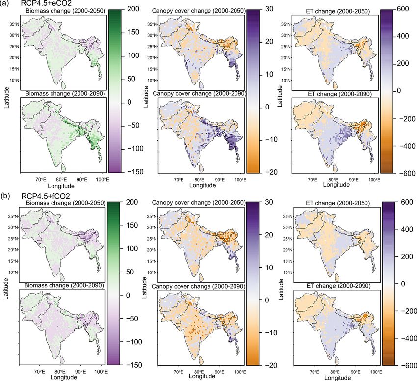
2958                                                    D. Kumar et al.: Climate change impact on South Asian vegetation

It is therefore of vital importance to understand how ecosys-    opment, land surface temperature and groundwater recharge
tems respond to simultaneous increases in atmospheric CO2        (Fisher et al., 2011).
and temperature, to changes in precipitation regime, and to         South Asia is home to approximately 1.7 billion people
altered ecosystem water balance in order to avoid critical       and is one of the regions most vulnerable to climate change
ecosystem disruptions and the resulting consequences for         (Eckstein et al., 2018). It hosts four of the world’s biodi-
biodiversity and humankind.                                      versity hotspots (Myers et al., 2000) and harbors different
   Increases in temperatures, decreases in precipitation and     biome types ranging from tropical in the south to temperate
changes in precipitation seasonality can cause loss of vege-     in the north at the fringe of the Himalayas. These hotspots
tation biomass. Plants using C3 photosynthetic pathway are       are characterized by high levels of diversity and endemism,
often not saturated at the current atmospheric CO2 , whereas     and they are threatened by climate change and anthropogenic
plants using the C4 photosynthetic pathways are already at       land use (Deb et al., 2017). For instance, woody encroach-
their physical optimum at current atmospheric CO2 levels         ment due to rising CO2 threatens South Asian savannas (Ku-
(Ehleringer and Cerling, 2002). The physiology of C3 plants      mar et al., 2020), and sifting cultivation in the northeastern
implies that elevated atmospheric CO2 improves their abil-       part of South Asia threatens biodiversity (Bera et al., 2006).
ity for carbon uptake due to the CO2 fertilization (Woodrow         Due to the absence of long-term field experiments such
and Berry, 1988) and enhances carbon sequestration (Leakey       as FACE experiments, in the dominant biomes of the region,
et al., 2009; Norby and Zak, 2011) as well as plant water        modeling studies are valuable tools to close existing knowl-
use efficiency (Soh et al., 2019). This has also been observed   edge gaps. Dynamic global vegetation models (DGVMs,
in long-term free-air carbon dioxide enrichment (FACE) ex-       Prentice et al., 2007) are particularly well suited to address
periments (Norby and Zak, 2011). Thus, elevated CO2 in-          questions that focus on vegetation response to changing envi-
fluences photosynthesis and thereby affects other physio-        ronmental drivers, e.g., climate and CO2 . While most DGVM
logical processes such as respiration, decomposition (Do-        studies in South Asia focused on the vulnerability of forests
herty et al., 2010), evapotranspiration (ET) and biomass ac-     to climate change (Chaturvedi et al., 2011; Ravindranath
cumulation (Frank et al., 2015). Increasing CO2 concentra-       et al., 2006, 1997), they often overlooked the severely threat-
tion has been associated with woody cover increase in struc-     ened savanna biome. These studies were further limited by
turally open tropical biomes such as grasslands and savan-       the utilization of models with fixed ecophysiological param-
nas (Stevens et al., 2017). This widespread proliferation of     eters and traits, e.g., fixed carbon allocation values to as-
woody plants into arid and semiarid ecosystems has been at-      sign carbon to plant biomass pools, fixed specific leaf area
tributed to increased water use efficiency in C3 plants that     (SLA) and pre-defined bioclimatic limits that were derived
facilitates woody sapling establishment and growth due to        from contemporary climatology in order to constrain the
higher drought tolerance (Kgope et al., 2010; Stevens et al.,    spatial distribution of plant functional types (PFTs). More-
2017). These CO2 effects on plant growth and competition         over, many DGVMs used in these studies do not account for
can alter community structure (height distribution), ecosys-     life history, eco-evolutionary processes and trait variability
tem productivity, climatic niches of ecosystems and biome        among individual plants (Kumar and Scheiter, 2019). While
boundaries (Nolan et al., 2018; Wingfield, 2013). Change         some global-scale studies have investigated the potential ef-
in vegetation distribution and altered vegetation structure      fect of increasing CO2 on natural vegetation, carbon seques-
feed back on climate by altering fluxes of energy, moisture,     tration and biome boundaries (e.g., Hickler et al., 2006; Sato
and CO2 between land and atmosphere (Friedlingstein et al.,      et al., 2007; Smith et al., 2014), detailed modeling studies fo-
2006). Feedback mechanisms also involve vegetation-medi-         cusing explicitly on different biomes in South Asia have not
ated changes in albedo, surface roughness, land--atmosphere      been conducted. The physiological effects of increased CO2
fluxes and evapotranspiration (Field et al., 2007; Richardson    and climate change on South Asian vegetation are uncertain
et al., 2013).                                                   and need to be addressed in order to improve understanding
   Enhanced plant growth due rising CO2 implies rapid leaf       of regional ecosystem functioning as well as implications for
area development and more total leaf area could translate into   biodiversity conservation.
higher transpiration (Leakey et al., 2009). However, elevated       To address the knowledge gaps in existing studies, we used
CO2 concentrations may decrease leaf stomatal conductance        the aDGVM2 (adaptive dynamic global vegetation model
to water vapor, which could reduce transpiration. Evapotran-     version 2), an individual- and trait-based vegetation model
spiration (ET) is a key ecophysiological process in the soil–    that combines elements of traditional DGVMs (Prentice
vegetation–atmosphere continuum (Feng et al., 2017). An-         et al., 2007) with newly implemented approaches for se-
nually, 64 % of the total global land-based precipitation is     lection and trait filtering. In aDGVM2, environmental con-
returned to the atmosphere through ET (Zhang et al., 2016).      ditions select for the plants with trait value combinations
Environmental change and concurrent vegetation changes al-       that make them successful under these conditions. There-
ter ET and affect water availability (Mao et al., 2015), es-     fore, plant communities that are adapted to site-specific en-
pecially in arid and semiarid regions. In these regions, ET      vironmental conditions dynamically assemble and emerge
affects surface and subsurface processes such as cloud devel-    as a reaction to the environmental forcing (Langan et al.,

Biogeosciences, 18, 2957–2979, 2021                                                 https://doi.org/10.5194/bg-18-2957-2021
D. Kumar et al.: Climate change impact on South Asian vegetation                                                            2959

2017; Scheiter et al., 2013). Originally, aDGVM2 had been          et al., 2018; Sinha et al., 2018). South Asia hosts four ma-
tested for Amazonia (Langan et al., 2017) and Africa (Gail-        jor global biodiversity hotspots, namely the Western Ghats,
lard et al., 2018; Pfeiffer et al., 2019). In order to adapt it    Himalayas, India and Myanmar, and Sri Lanka (Myers et al.,
to South Asian ecosystems and their diversity, we included         2000). These hotspots include a wide diversity of ecosystems
C3 grasses, improved ecophysiological processes such as the        such as mixed wet evergreen, dry evergreen, deciduous and
leaf energy budget in order to estimate leaf temperature, im-      montane forests. Further vegetation types are alluvial grass-
plemented separate temperature sensitivities for C3 and C4         lands and subtropical broadleaf forests along the foothills
photosynthetic capacity (Vcmax ), and included snow in the         of the Himalayas, temperate broadleaf forests in the mid-
water balance model.                                               hills, mixed conifer and conifer forests in the higher hills,
   In this study we used the updated version of aDGVM2 and         savanna in the Deccan region and southern part of Malaysia,
addressed the following questions:                                 and alpine meadows above the tree line.

    1. How do projected changes in climate and CO2 follow-         2.2   Model description
       ing two representative concentration pathways (RCP8.5
       and RCP4.5, Meinshausen et al., 2011) change the dis-       For this study we used aDGVM2 (Scheiter et al., 2013; Lan-
       tribution, boundaries and climatic niches of biomes in      gan et al., 2017; Gaillard et al., 2018), a DGVM with a dy-
       South Asia?                                                 namic trait approach. In the Supplement we summarize main
                                                                   features of aDGVM2 and explain how the physiological ef-
    2. How does the relationship between projected biomass,        fects of changing CO2 concentration and rising temperature
       ET, temperature and precipitation change in response to     are simulated in a process-based way in the aDGVM2 by the
       CO2 fertilization?                                          implemented photosynthesis routine. To adapt the aDGVM2
                                                                   to the requirements of the study region, we incorporated new
    3. What is the sensitivity of predicted changes in relation    subroutines into the model. We improved the representation
       to presence and absence of CO2 fertilization?               of (a) the water balance by including snow, (b) the carboxy-
                                                                   lation rate, and (c) leaf temperature, and (d) we included C3
Based on our results we analyzed climate–vegetation inter-         grasses (previous model versions only simulated C4 grasses).
actions to improve our understanding of how to manage and
mitigate impacts on biomes under climate change and in-              a. Water balance.
creasing CO2 .                                                           In aDGVM2, the soil water module is based on the
                                                                         tipping-bucket concept. As the model was originally de-
                                                                         veloped with a strong focus on tropical and subtropi-
2     Methods                                                            cal forest and savanna regions, the original model ver-
                                                                         sion only considered water input in the form of rain
2.1    Description of the study region
                                                                         (see Langan et al., 2017). In the updated model ver-
                                                                         sion, precipitation is assigned as snow when daily mean
Approximately 1.7 billion people populate South Asia, i.e.,
                                                                         air temperature drops below 0 ◦ C. Snow accumulates
the Indian subcontinent, Afghanistan and Myanmar. South
                                                                         on the soil surface or is added on top of an existing
Asia incorporates a wide range of bioclimatic zones with dis-
                                                                         snowpack. The snowpack persists as long as air tem-
tinctive biomes, ecosystem types and species (Rodgers and
                                                                         perature remains below 0 ◦ C. Once temperature rises
Panwar, 1988). Climatic conditions are controlled by inter-
                                                                         above 0 ◦ C, water from snowmelt is added to the soil
actions between the South Asian summer monsoon system
                                                                         water pool and becomes available to plants. This pro-
and the region’s complex topography. The climatic enve-
                                                                         cess may improve the water availability for plants at the
lope ranges from tropical arid and semiarid regions in the
                                                                         beginning of spring, for example in the Himalayan re-
west to humid tropical regions supporting rain forests in the
                                                                         gion. Snowmelt (Smelt , mm/day) is calculated following
northeast and temperate vegetation at the fringe of the Hi-
                                                                         Choudhury et al. (1998) as
malayas. Excluding the Himalayan regions, South Asia has a
mean annual temperature of approximately 24 ◦ C with very                Smelt = 1.5 + Km Pprecip (Ta − Tsnow )Spack ,         (1)
low spatial variability. Mean annual precipitation (MAP) is
1190 mm, ranging from less than 500 mm in the warm desert                where Km is the coefficient of snowmelt
zone in the west to more than 3500 mm in the northeast. The              (0.007 mm/day/◦ C), Spack is the depth of the snowpack
steep elevation gradients ranging from sea level to 8800 m               (mm) and is equivalent to the accumulated solid portion
result in a rich diversity of ecosystems that can alternate in           of precipitation, Ta is the daily mean air temperature
areas of a few hundred square kilometers. Topography is rec-             (◦ C), Pprecip is precipitation (mm/day), and Tsnow is
ognized as a strong driver of ecological patterns, for example           the maximum temperature where precipitation falls as
those related to forest structure and composition, floristic di-         snow (0 ◦ C). We do not consider insulation effects of
versity and soil fertility (Gallardo-Cruz et al., 2009; Jucker           the snowpack in the model.

https://doi.org/10.5194/bg-18-2957-2021                                                    Biogeosciences, 18, 2957–2979, 2021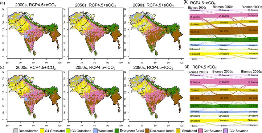
2960                                                     D. Kumar et al.: Climate change impact on South Asian vegetation

 b. Carboxylation rate.                                                as
    In earlier versions of aDGVM2, leaf-level photosyn-                                    Vcmax,25 20.1(Tleaf −25)
    thesis was calculated at the population level; i.e., it            Vcmax =                                                      ,   (4)
                                                                                 (1 + e0.3(Tlow −Tleaf ) )(1 + e0.3(Tleaf −Tupp ) )
    was assumed that all plants of a simulated vegetation
    stand have the same leaf-level photosynthetic rate. Only           where Tleaf is the leaf temperature in ◦ C (see next para-
    C3 - and C4 -type photosynthesis were distinguished. We            graph for calculation). The photosynthetic model of
    therefore implemented new routines to calculate photo-             Collatz et al. (1992) and Collatz et al. (1992) assumes
    synthesis at a daily time step for each individual plant.          specific values of Tupp and Tlow for C3 and C4 plants, re-
    We further incorporated an empirical relation between              spectively (Tables S1 and S2 in the Supplement). These
    specific leaf area (ASLA , mm2 /mg) and leaf nitrogen              temperature ranges from −10 to 36 ◦ C and from 13
    content per unit area (Na , g/m2 ) following Sakschewski           to 45 ◦ C for C3 and C4 photosynthetic pathways, re-
    et al. (2015):                                                     spectively, allow plants to grow most efficiently in their
                                                                       plant-specific climatic niches.
    Na = 6.89A−0.571
              SLA .                                         (2)
                                                                    c. Leaf temperature.
    The standard maximum carboxylation rate of ru-
                                                                       We calculate leaf temperature following the leaf-level
    bisco per leaf area (Vcmax,25 , µmol/m2 /s) was derived
                                                                       energy budget concept (Gates, 1968). Leaf-level pho-
    from the TRY database (Kattge and Knorr, 2007) by
                                                                       tosynthesis, activity of leaf enzymes and transpiration
    Sakschewski et al. (2015) and is calculated as
                                                                       depend on leaf temperature (Tleaf , ◦ C), calculated as
    Vcmax,25 = 31.62Na0.501 ,                               (3)
                                                                                        Rn − λErgb

                                                                       Tleaf = Tair +                 ,                        (5)
    where Vcmax,25 is Vcmax at 25 ◦ C. In the model, ASLA is                               ρCP
    linked to the matric potential at 50 % loss of xylem con-          where Tair is air temperature (◦ C), Rn is net radiation
    ductance (P50; see Langan et al., 2017). The trade-off             absorbed by the leaf (MJ/m2 /day), λ is latent heat of
    between ASLA and Vcmax mediated by leaf traits (Na )               vaporization (MJ/kg), E is evapotranspiration (m/day),
    introduces variability in the spectrum of tree growth              rgb is the boundary layer resistance (m/s), ρ is the
    strategies in aDGVM2. ASLA is linked to leaf longevity             air density (kg/m3 ) derived from atmospheric pressure
    (LL) in aDGVM2, such that it affects the leaf turnover             (101.325 kPa at sea level) that is scaled according to the
    rates (represented by Eq. 72, in Appendix, Langan et               elevation and Tair , and CP is the specific heat of dry air
    al., 2017). Leaves with high ASLA have shorter LL and              (MJ/kg/◦ C). Leaf temperature is used to calculate the
    higher turnover rates than leaves with low ASLA (and               temperature dependence of Vcmax used in the photosyn-
    vice versa). The correlation between ASLA , P50 and LL             thesis model routines in Eq. (4). Absorbed net radia-
    represents the trade-off between two opposing resource             tion (Rn ), rgb and E are model state variables calculated
    strategies, i.e., conservation vs. rapid acquisition of soil       from climate input used in aDGVM2 (Tair , long-wave
    water and nutrients (Wright et al., 2005). Trees that in-          and shortwave radiation, and ρ). The values of latent
    vest more carbon into their leaves (low ASLA ) enhance             heat of vaporization (λ) and CP are 2.45 MJ/kg and 2.71
    their structural stability but have lower leaf turnover to         MJ/kg/◦ C, respectively, and are assumed to be constant
    mitigate the higher initial carbon investment.                     parameters in this model version.
    The effect of temperature on photosynthesis is well
    described (Kirschbaum, 2004), and temperature may               d. C3 grasses.
    influence photosynthesis both directly, via tempera-               C3 grasses were not included in previous aDGVM2 ver-
    ture dependency of enzyme-mediated metabolic rates                 sions (Gaillard et al., 2018; Langan et al., 2017; Pfeif-
    of carboxylation and the Calvin cycle (Sharkey et al.,             fer et al., 2019; Scheiter et al., 2013). We therefore im-
    2007), and indirectly, via its effect on transpiration             plemented C3 grasses, following the approach used for
    and plant water uptake and transport (Urban et al.,                C4 grasses in previous model versions, but adjusted the
    2017). The maximum carboxylation rate (Vcmax ) in-                 photosynthetic pathway (see Appendix S2 in Langan
    creases with temperature until it reaches an optimum,              et al., 2017). C3 and C4 grasses use a different leaf-level
    and it decreases again at temperatures above the opti-             photosynthesis model (Farquhar et al., 1980) follow-
    mum (Kattge and Knorr, 2007) due to reductions in en-              ing the implementations of Collatz et al. (1991, 1992).
    zyme activity. Above 30 ◦ C the electron transport chain           The optimum temperature ranges for carboxylation for
    is gradually inhibited, and at temperatures above 40 ◦ C           C3 and C4 grasses are also different (Table S1). As C3
    the denaturation of rubisco and associated proteins be-            grasses have higher cold tolerance than C4 grasses (Liu
    comes relevant (Lloyd et al., 2008). The temperature de-           and Osborne, 2008), we implemented frost intolerance
    pendency of the carboxylation rate (Vcmax ) is expressed           for C4 grasses but not for C3 grasses. Frost is assumed

Biogeosciences, 18, 2957–2979, 2021                                                   https://doi.org/10.5194/bg-18-2957-2021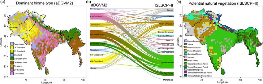
D. Kumar et al.: Climate change impact on South Asian vegetation                                                            2961

      to damage the tissue of C4 grasses, and in aDGVM2 we       2009) and include information on soil properties and
      kill 10 % of the living leaf biomass of C4 grasses per     types. The soil properties include parameters required by
      frost day independent of frost severity.                   aDGVM2: volumetric water-holding capacity, soil hydraulic
                                                                 conductivity, soil bulk density, soil depth, soil texture, soil
2.3     Model forcing data                                       carbon content, soil wilting point and field capacity (for de-
                                                                 tails see Fig. S3b and Langan et al., 2017). A digital el-
2.3.1    Climate data                                            evation model (DEM) at 90 m spatial resolution was ob-
                                                                 tained from the Shuttle Radar Topography Mission (SRTM,
We used GFDL-ESM2M climate data for the period 1950 to
                                                                 Fig. S3a http://srtm.csi.cgiar.org, last access: March 2016,
2099 from the Inter-Sectoral Impact Model Inter-comparison
                                                                 Jarvis et al., 2008). It was resampled to a spatial resolution of
Project (ISIMIP2), as historical climate simulated by GFDL-
                                                                 0.5◦ × 0.5◦ to match the spatial resolution of climate data. In
ESM2M showed satisfactory performance for South Asia
                                                                 the model, elevation is used to calculate the surface pressure
(McSweeney and Jones, 2016). The general circulation
                                                                 at a given altitude, which is used to scale up air density and
model (GCM) output was bias-corrected in the Inter-Sectoral
                                                                 partial pressure of oxygen. The partial pressure of oxygen is
Impact Model Intercomparison Project (ISIMIP) and down-
                                                                 used to estimate the CO2 compensation point of photosyn-
scaled to a spatial resolution of 0.5◦ × 0.5◦ (Warszawski
                                                                 thesis (Eq. 2 of Appendix S2 in Langan et al., 2017). We did
et al., 2014). We used average, maximum and minimum air
                                                                 not use slope and aspect in the model.
temperatures, precipitation, surface downwelling shortwave
radiation and long-wave radiation, near-surface wind speed,
                                                                 2.4   Model simulation protocol
and relative humidity at a daily temporal resolution. We used
two representative concentration pathways, namely RCP4.5
                                                                 To understand how climate and CO2 fertilization interact to
and RCP8.5 (Meinshausen et al., 2011). These scenarios as-
                                                                 influence the future vegetation state in South Asia, we sim-
sume increases in radiative forcing of 4.5 and 8.5 W/m2 by
                                                                 ulated all combinations of two climate scenarios (RCP4.5
2100 (Van Vuuren et al., 2011) and increases in atmospheric
                                                                 and RCP8.5) and two CO2 scenarios (CO2 fertilization en-
CO2 concentrations to 560 and 970 ppm by 2100, respec-
                                                                 abled or disabled, four scenarios in total). We simulated po-
tively (Van Vuuren et al., 2011).
                                                                 tential natural vegetation between 1950 and 2099 using daily
                                                                 climate data for RCP4.5 and RCP8.5 (see Sect. 2.3.1). For
2.3.2    Projected changes in temperature and
                                                                 both scenarios, simulations were run with a CO2 increase
         precipitation
                                                                 in line with RCP4.5 (hereafter RCP4.5+eCO2 ) and RCP8.5
Mean annual precipitation (MAP) from GFDL-ESM2M does             (hereafter RCP8.5+eCO2 ) and with the same climate data
not show a clear trend when averaged for South Asia un-          but fixed CO2 after 2005 at 375 ppm for RCP4.5 (hereafter
der RCP4.5 and RCP8.5, due to high inter-annual variabil-        RCP4.5+f CO2 ) and RCP8.5 (hereafter RCP8.5+f CO2 ).
ity of precipitation (Fig. S1 in the Supplement). Yet, there     Fixing the CO2 concentration after 2005 mimics a situation
are region-specific differences in precipitation change. The     where CO2 fertilization would not occur and vegetation only
Western Ghats which are located between 73–77◦ E and 8–          responds to the climate signal. All simulations were con-
21◦ N and the eastern Himalayan region are projected to be-      ducted with natural fire as implemented in aDGVM2 and at
come wetter under both RCP4.5 and RCP8.5, whereas the            0.5◦ × 0.5◦ spatial resolution. The aDGVM2 simulates 1 ha
western part of the region is projected to become drier by       stands that are assumed to be representative for the vege-
the end of the century under both RCPs (Fig. S2). MAP is         tation at a larger scale; i.e., we assume that the stand-level
projected to increase by more than 600 mm in the eastern         vegetation homogeneously covers the grid cell. The “repre-
Himalayas and Western Ghats but predicted to decrease by         sentative hectare approach” is a concession to computational
400–600 mm in the western and central area of the region         limitation, as photosynthesis and physiological processes are
(Fig. S2). By the end of the 21st century, the mean annual       simulated individually for all individual plants of a stand (up
temperature (MAT) of South Asia is expected to increase          to 36 000 individuals). It balances adequate representation of
between ca. 1 and 3.5 ◦ C under RCP4.5 and between 1 and         trait diversity among individuals against computational con-
6 ◦ C under RCP8.5, relative to the average temperature in the   straints. Also due to computational constraints, we did not
baseline period of 2000–2009 (Figs. S1 and S2). The west-        conduct replicate simulations.
ern parts of the region and the Himalayan mountains are pro-        To ensure that simulated vegetation had sufficient time to
jected to experience higher increases in temperature than the    adapt to prevailing environmental conditions, we conducted
rest of the region (Fig. S2).                                    simulations for 650 years, split into a 500-year spin-up phase
                                                                 and a 150-year transient phase. For the spin-up phase, we
2.3.3    Soil and elevation data                                 randomly sampled years of the first 30 years of daily climate
                                                                 data (1950 to 1979). For the transient phase, we used the se-
Soil data were obtained from FAO (http://www.fao.org/            quence of daily climate data between 1950 and 2099. Trial
soils-portal, last access: March 2016, Nachtergaele et al.,      simulations showed that a 500-year spin-up period is suffi-

https://doi.org/10.5194/bg-18-2957-2021                                                 Biogeosciences, 18, 2957–2979, 2021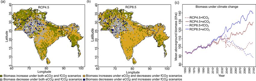
2962                                                     D. Kumar et al.: Climate change impact on South Asian vegetation

cient to ensure that vegetation is in a dynamic equilibrium       canopy cover greater than 45 % were classified as forest if
state with environmental drivers.                                 tree cover exceeded shrub cover or shrubland if shrub cover
                                                                  exceeded tree cover, irrespective of grass biomass. Forests
2.5    Model benchmarking and evaluation                          were subdivided into evergreen and deciduous forest based
                                                                  on the dominance of canopy area of both tree phenology
For benchmarking of aDGVM2 simulation results, we used            types. In aDGVM2, whether a plant is deciduous or ever-
five different remote sensing products: aboveground biomass       green is decided by a trait. Biomes considered in this study
(t/ha, Saatchi et al., 2011), tree height (m, Simard et al.,      were hence C3 grassland, C4 grassland, shrubland, wood-
2011), tree cover (percent, Friedl et al., 2010), MODIS evap-     land, deciduous forest, evergreen forest, C3 savanna and C4
otranspiration (mm/year, Zhang et al., 2010) and natural veg-     savanna.
etation type (Ramankutty et al., 2010). We used a 10-year            Biomes differ in the amount of precipitation they receive
average of MODIS ET and compared it to a 10-year average          and their temperatures. Whittaker plots describe the bound-
of model-simulated ET (mm/year; 2000–2009). All remote            aries of observed biomes with respect to temperature and
sensing data sets were aggregated to a 0.5◦ × 0.5◦ spatial res-   precipitation. We used the “plotbiomes” R package (https:
olution to match the spatial resolution of model simulations      //github.com/valentinitnelav/plotbiomes by                ) to
by calculating the mean of all values within each 0.5◦ grid       create Whittaker plots based on Ricklefs (2008) and Whit-
cell or using nearest-neighbor aggregation in the case of veg-    taker (1975). We overlaid the simulated biomes on Whittaker
etation type (“raster” package in R, Hijmans and van Etten,       plots to assess climatic niches of biomes under current cli-
2012). We first compared model results and observations as-       mate to determine shifts in climatic niches by the end of this
suming that the entire study region is covered by natural veg-    century as a result of climate change and elevated CO2 under
etation (Fig. 1). Then we repeated the comparisons only for       both RCPs (see Sect. 3.6).
areas with predominantly natural cover; i.e., we masked out
areas with more than 50 % managed land (Fig. S4, land cover       2.7   Calculation of biome-level evapotranspiration
classes 7 “Cultivated and Managed Vegetation” and 9 “Urban
and Built-up” in Tuanmu and Jetz, 2014). We calculated the        For analyzing evapotranspiration change we calculated the
normalized mean squared error (NMSE) and coefficient of           amount of water transpired per unit leaf biomass. Simu-
determination (R 2 ) to quantify agreement between data and       lated ET and leaf biomass for woody plants, C3 grass, and
simulated variables.                                              C4 grass were summed and scaled to the grid level, tak-
                                                                  ing latitudinal variation of grid cell area into account. Ab-
2.6    Biome classification                                       solute change in evapotranspiration quantity can either re-
                                                                  sult from the change in biome area, from a change in total
The aDGVM2 simulates state variables such as biomass and          amount of leaf biomass over time or from changes in wa-
canopy cover of individual plants in simulated vegetation         ter use efficiency. In order to eliminate the effects caused by
stands (1 ha, which is a representative of a grid cell). We       change in biome area and leaf biomass, we calculated biome-
used woody canopy area, abundance of shrubs and trees,            level evapotranspiration by normalizing evapotranspiration
and grass biomass to classify the simulated vegetation into       with biome-level leaf biomass (Eq. 6). Due to the normal-
biome types (Fig. S5). We used 10-year averages of state          ization, differences in evapotranspiration at the biome level
variables for the periods 2000–2009, 2050–2059 and 2090–          are comparable between different biomes and independent
2099 to represent the 2000s, 2050s and 2090s, respectively.       from biome attributes such as spatial extent and biome-level
We classified areas with woody canopy cover below 5 % as          biomass. The biome-level evapotranspiration is calculated as
barren if grass biomass was below 100 kg/ha and as grass-         the ratio of total annual ET over total leaf biomass for all
land if grass biomass exceeded 100 kg/ha. Grassland was           respective biomes:
classified as C3 grassland or C4 grassland based on predom-                 PG
inance of C3 or C4 grass biomass. Simulated woody individ-                         (Egrid,i Agrid,i )
                                                                  Ebiome = Pi=1
                                                                            G
                                                                                                        ,                       (6)
uals were classified as trees if they had three or less stems                  i=1 (Bgrid,i Agrid,i )
and as shrubs if they had four or more stems (see Supple-
ment). The canopy cover of woody plants and grass biomass         where Ebiome is biome-level ET (mm/kg/year), 1, 2, . . . , G
was used to separate woodland and savanna biomes. Grid            represents the grid cells of the biome; Agrid,i is the area of
cells with tree canopy cover greater than shrub canopy cover,     grid cell i (m2 ); Egrid,i is the total evapotranspiration of grid
tree canopy cover between 5 % and 45 %, and grass biomass         cell i (mm/year); and Bgrid,i is the leaf biomass of grid cell
below 100 kg/ha were classified as woodland. Grid cells           i (kg/m2 ). Choosing to normalize evapotranspiration to leaf
with the same woody cover characteristics but grass biomass       biomass integrates over both increased water use efficiency
higher than 100 kg/ha were classified as savanna. Savanna         and soil water availability constraints. It is therefore suitable
was further separated into C3 savanna and C4 savanna based        to characterize overall change in the water balance over time
on the predominance of C3 or C4 grass biomass. Areas with         at the biome level, as it not only indicates water used to pro-

Biogeosciences, 18, 2957–2979, 2021                                                  https://doi.org/10.5194/bg-18-2957-2021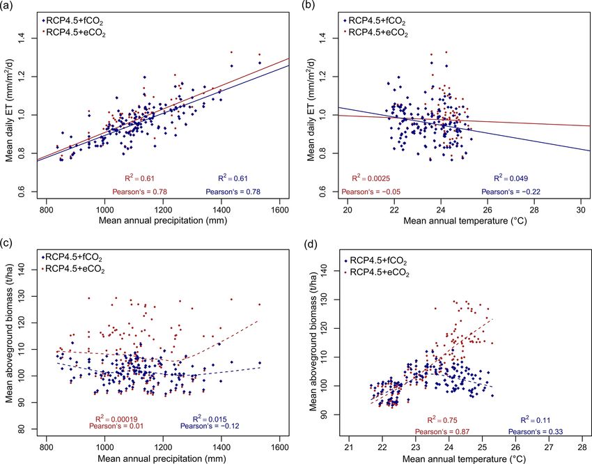
D. Kumar et al.: Climate change impact on South Asian vegetation                                                                         2963

Figure 1. Comparison between aDGVM2 results and data for (a) simulated biomass and Saatchi et al. (2011) biomass, (b) simulated tree
height and Simard et al. (2011) tree height, (c) simulated tree cover and Friedl et al. (2011) tree cover, and (d) simulated evapotranspiration
and Zang et al. (2010) evapotranspiration. In the figure the first column shows the remote sensing products, the second column shows
aDGVM2 results, the third column shows the difference between simulation and data, and the fourth column shows the scatter plot between
simulated state variables against benchmarking data. NMSE and RMSE are the normalized mean square error and root mean square error,
respectively. In the fourth column, each point represents one grid cell in the study region. For results with masked land-use cover see
Supplement Fig. S4.

duce new biomass (as gross primary production over tran-                  3     Results
spiration would express), but also includes water required
to sustain existing biomass. We calculated the percentage                 3.1    Model performance and contemporary vegetation
change in Ebiome for respective scenarios between the 2010s                      patterns
and 2050s and between the 2010s and the 2090s.
                                                                          The aDGVM2 captured contemporary large-scale patterns
                                                                          of biomass, canopy cover, tree height and evapotranspira-
                                                                          tion. Model results agreed well with remote sensing prod-

https://doi.org/10.5194/bg-18-2957-2021                                                            Biogeosciences, 18, 2957–2979, 2021
2964 D. Kumar et al.: Climate change impact on South Asian vegetation
Figure 2. Comparison between simulated and observed biome patterns. (a) Simulated dominant biome type, (b) Sankey diagram showing
overlap between simulated biomes and potential natural vegetation cover (ISLSCP II, Ramankutty et al., 2010), and (c) potential natural
vegetation. The Sankey graph shows how aDGVM2 biomes and PNV classes overlap.
ucts used for benchmarking (Figs. 1 and 2). R 2 was 0.61, and CO2 and hence changes in biome type, predominantly
0.45, 0.6 and 0.71, and NMSE was 0.48, 0.78, 0.4 and 1.07 from savanna and grassland to deciduous forest (Fig. 3a,
for biomass (Saatchi et al., 2011), tree height (Simard et al., b). Simulations showed an increase in the area covered
2011), tree cover (Friedl et al., 2010) and evapotranspira- by evergreen and deciduous forests under both scenarios
tion (Zhang et al., 2010), respectively (Fig. 1). Data–model with eCO2 , in contrast to simulations under both scenar-
agreement improved when masking out managed land (Tu- ios with f CO2 , where CO2 was fixed after 2005 (Ta-
anmu and Jetz, 2014). R 2 increased to 0.66, 0.71, 0.67 and ble 1). Under RCP4.5+eCO2 , evergreen and deciduous for-
0.80, while NMSE decreased to 0.43, 0.30, 0.61 and 1.03 est cover increased by 3.1 % and 21.2 % until the 2050s and
for biomass, tree height, tree cover and evapotranspiration, by 38.0 % and 59.1 % until the 2090s, respectively. Under
respectively (Fig. S4). The model performed well in areas RCP8.5+eCO2 , evergreen and deciduous forest increased
with higher fractional cover of natural vegetation, such as by 24.8 % and 45.4 % until the 2050s and by 46.5 % and
the Himalayas, Western Ghats and the northeast of the re- 60.2 % until the 2090s, respectively. The model simulated
gion, although the model overestimated biomass and canopy a small increase in forest area for RCP4.5+f CO2 , where
area in the Brahmaputra basin, which lies between 28–34◦ N the area increased by 7.9 % and 14.4 % for evergreen and
and 90–96.5◦ E in the northeast of the study region (Fig. 1a, deciduous forest until the 2090s, respectively. Evergreen
c, Kumar et al., 2020). forests were mainly simulated along the Himalayas, West-
The model simulated evergreen forests along the Hi- ern Ghats and eastern parts of the study region under current
malayan mountains, the southern part of the Western Ghats conditions (2000s, Fig. 3a) but expanded into the south of
and Sri Lanka, whereas deciduous forest was simulated in the peninsular India in future periods (2050s and 2090s) under
northern Western Ghats, central India and the southern parts RCP4.5+eCO2 . Deciduous forest cover also increased in fu-
of Myanmar (Fig. 2a). Savanna was simulated in the south- ture periods in central India and along the Himalayas (Figs. 3
ern, northern, and western parts of India and some regions of and S6).
central Myanmar. Shrublands were simulated in the arid re- The extent of C4 savanna showed a significant decrease
gions of Pakistan, the western parts of India and Afghanistan. under scenarios with eCO2 , although in RCP4.5+eCO2 it
The aDGVM2 simulated woodland in the west of central In- showed an increase by 12.1 % between the 2010s and the
dia and grassland in the drier regions (Fig. 2a). A large pro- 2050s (Table 1, Fig. 3). Simulated C4 savanna area de-
portion of simulated deciduous forest area is in good agree- creased by 14.1 % relative to the 2000s until the 2090s under
ment with that in maps of potential natural vegetation (PNV, RCP4.5+eCO2 . Under RCP8.5+eCO2 the model projected
Fig. 2b, c). However a large proportion of simulated savanna a decrease in C4 savanna area of 21.6 % and 32.2 % until the
area is represented as deciduous forest in the map of PNV 2050s and the 2090s, respectively. The area covered by C4
(Fig. 2b). savanna increased under both RCPs with f CO2 (Table 1).
C4 savannas were mainly located in the northern plain and
3.2 Projected changes in biome distribution pattern peninsular India in the baseline period. However, these areas
were replaced by deciduous forests in the northern plain and
The aDGVM2 projected increasing trends for canopy cover central India and by evergreen forests in peninsular India and
and aboveground biomass in response to climate change in the southeast of the region by the 2090s under eCO2 sce-
Biogeosciences, 18, 2957–2979, 2021 https://doi.org/10.5194/bg-18-2957-2021D. Kumar et al.: Climate change impact on South Asian vegetation 2965
Table 1. Biome cover (in %) for the 2000s, 2050s and 2090s, and percent (%) change in biome cover from the 2000s to the 2050s and the
2000s to the 2090s under RCP4.5 and RCP8.5 with fixed and elevated CO2 . 1 indicates percent change in biome cover between time periods.
RCP scenarios Year
C4 grassland
C3 grassland
C4 savanna
C3 savanna
Evg. forest
Dec. forest
Shrubland
Woodland
Barren
RCP4.5+f CO2 2010s 5.6 15.4 4.6 18.2 11.7 17.6 6.9 17.7 2.4
2050s 6.3 14.8 3.2 15.7 11.2 18.6 6.7 22.1 1.4
2090s 10.4 12.3 2.3 10.0 12.7 20.1 6.0 24.7 1.4
1 2050s–2010s 13.0 −3.7 −32.2 −13.6 −4.0 5.6 −3.0 25.4 −39.1
1 2090s–2010s 87.0 −20.1 −50.0 −45.2 7.9 14.4 −12.7 40.1 −41.3
RCP4.5+eCO2 2010s 5.7 15.2 4.8 18.6 11.5 17.5 6.8 17.5 2.4
2050s 6.5 13.9 3.5 15.0 11.9 21.2 7.0 19.6 1.3
2090s 10.4 10.4 2.5 10.7 15.9 27.9 6.2 15.1 0.9
1 2050s–2010s 13.5 −8.2 −26.9 −19.7 3.1 21.2 3.8 12.1 −44.7
1 2090s–2010s 82.0 −31.6 −48.4 −42.4 38.0 59.1 −8.4 −14.1 −63.8
RCP8.5+f CO2 2010s 6.3 14.7 4.5 18.8 11.7 17.3 6.3 18.0 2.4
2050s 8.8 12.3 2.5 14.7 12.9 21.7 6.6 19.0 1.5
2090s 9.4 15.0 2.5 11.0 10.8 14.2 6.7 29.0 1.4
1 2050s–2010s 39.0 −16.5 −43.7 −21.9 10.1 25.0 4.1 5.4 −39.1
1 2090s–2010s 48.8 1.8 −43.7 −41.6 −7.9 −17.9 5.7 61.0 −41.3
RCP8.5+eCO2 2010s 5.9 14.8 4.7 18.0 11.6 17.5 7.1 17.9 2.5
2050s 9.7 10.5 3.2 13.9 14.5 25.4 7.1 14.1 1.6
2090s 6.3 11.5 4.2 12.6 17.0 28.0 7.0 12.2 1.3
1 2050s–2010s 64.9 −29.5 −32.6 −22.9 24.8 45.4 0.7 −21.6 −35.4
1 2090s–2010s 7.0 −22.2 −10.9 −30.3 46.5 60.2 −1.5 −32.2 −47.9
narios (Figs. 3a and S6a). The model simulated a decrease malayas, as well as in the central, northeastern and western
in area covered by woodland, shrubland, grasslands and C3 parts of the study region by the end of the century. Mod-
savanna by the 2090s under all scenarios (Table 1, Fig. 3). eled biomass decrease is higher under RCP8.5 in these re-
Simulations showed an increase in barren areas in the west- gions (Figs. 4 and S7). Biomass in the central and south-
ern part of the region under all scenarios (Figs. 3 and S6, eastern part of the region is projected to increase under both
Table 1). RCPs with eCO2 until the 2050s and 2090s and to decrease
in southern India and in parts of western South Asia (Figs. 4
3.3 Projected changes in biomass at the biome level and S7). We found increased biomass in Afghanistan, west-
ern Pakistan, Nepal, and the southern part of Myanmar and
The aDGVM2 predicted an increase in mean biomass for decreased biomass in the western arid part of the study re-
evergreen and deciduous forest in the eCO2 scenarios for gion under both RCPs for both eCO2 and f CO2 (Fig. 5),
both RCPs (Table 2). Under RCP4.5+eCO2 , mean above- though the magnitude of change is different (Figs. 4 and S7).
ground biomass in evergreen and deciduous forest increased There were few areas in the western part of the study re-
by 8.1 % and 14.4 % by the 2050s and 3.8 % and 15.7 % gion where the model predicted increased biomass only un-
by the 2090s, relative to the baseline period. The increase der f CO2 for both RCPs (Fig. 5). In large parts of the study
is even higher under RCP8.5+eCO2 (Table 2). The mean region, biomass increased under eCO2 for both RCPs but
biomass of woodland decreased under both RCPs except for decreased under f CO2 ; that is, CO2 fertilization compen-
the 2050s with eCO2 scenarios. The mean biomass of grass- sates for climate-change-induced biomass diebacks in these
land increased under RCP4.5 but decreased for C4 grassland regions (Fig. 5).
under RCP8.5 for both f CO2 and eCO2 scenarios. Shrub-
lands in the western part of the study region showed an in- 3.4 Projected changes in evapotranspiration at the
crease in mean biomass under eCO2 scenarios except for biome level
the 2050s under both RCPs and a decrease under f CO2 for
both RCPs (Table 2). Our results showed that under RCP4.5 The response of simulated Ebiome varies in different biomes
and RCP8.5 biomass decreased in the areas along the Hi- under both RCP4.5 and RCP8.5 (Table 3). Under the
https://doi.org/10.5194/bg-18-2957-2021 Biogeosciences, 18, 2957–2979, 20212966 D. Kumar et al.: Climate change impact on South Asian vegetation
Figure 3. Simulated biome distribution for the 2000s, 2050s and 2090s under (a) RCP4.5+eCO2 and (c) RCP4.5+f CO2 . The Sankey
diagrams show the fractional cover of biomes and transitions between biomes from the 2000s to the 2050s and the 2050s to the 2090s under
(b) RCP4.5+eCO2 and (d) RCP4.5+f CO2 . See Fig. S6 for the simulated biome distribution under RCP8.5.
RCP4.5+f CO2 scenario the model predicted a decrease in (Figs. 4 and S7). We compared the spatially averaged annual
ET in all biomes except for deciduous forest and shrub- values over all of South Asia of simulated absolute ET with
land where it increased by 1 % and 2.1 % until the 2050s MAP over the period from 1951 to 2099 and found a stat-
and by 0.3 % and 11.9 % by the 2090s, respectively. Sim- ically significant relation (p value < 0.005). We found that
ulated Ebiome under RCP8.5+f CO2 for deciduous for- absolute ET was positively correlated with MAP under all
est and shrubland increased by 4.2 % and 5.2 % until four scenarios (Figs. 6a and S8a) but weakly correlated with
the 2050s and by 5.2 % and 16.4 % until the 2090s, re- MAT (Figs. 6b and S8b). For a given MAP, the spatially av-
spectively. The model also predicted increased Ebiome for eraged annual value of aboveground biomass (AGBM) was
C4 grassland, evergreen forest and C4 savanna until the lower in scenarios with f CO2 than scenarios with eCO2 un-
2090s under RCP8.5+f CO2 (Table 3). Comparisons of the der both RCPs (Figs. 6c and S8c). The spatially averaged an-
RCP4.5+f CO2 and RCP8.5+f CO2 scenarios indicated that nual value of AGBM decreased beyond a MAT of 23.5 ◦ C for
the former had a higher Ebiome than the latter scenario across both RCPs with f CO2 , whereas it increased beyond 23.5 ◦ C
all biomes because precipitation decrease is higher in the under both RCP scenarios with eCO2 (Figs. 6d and S8d).
RCP8.5 scenario than in the RCP4.5 scenario. Under both
RCPs with eCO2 , the model predicted a decrease in Ebiome
across all biomes, except for a marginal increase in shrub- 3.6 Impact of climate change on climatic niches of
land under RCP4.5 and deciduous forest under RCP8.5 un- biomes
til the 2050s and the 2090s (Table 3). In general, scenar-
ios with eCO2 showed lower biome-specific evapotranspira- The climate niches of simulated biomes broadly overlapped
tion across most of the biomes compared to simulations with with the biome niches in the Whittaker scheme (Figs. 7
f CO2 . and S9, Ricklefs, 2008; based on Whittaker, 1975). Under
RCP4.5+eCO2 and RCP8.5+eCO2 , the aDGVM2 simulated
3.5 Response of mean ET and mean aboveground shifts of climatic niches of biomes. Evergreen and decidu-
biomass to climate change ous forest biomes were predicted to invade the niche space
of savannas under eCO2 scenarios (Figs. 7 and S9). Savan-
The model predicted a larger increase in absolute annual nas in turn were predicted to expand their climatic niche to
mean ET (mm/year) under eCO2 than f CO2 for both RCP MAT > 30 ◦ C by 2099, a climatic space that was essentially
scenarios due to the corresponding increase in biomass not occupied by current biomes. Under RCP8.5+eCO2 in the
Biogeosciences, 18, 2957–2979, 2021 https://doi.org/10.5194/bg-18-2957-2021D. Kumar et al.: Climate change impact on South Asian vegetation 2967
Table 2. Mean biomass (in t/ha) within biomes for the 2000s, 2050s and 2090s, and percent (%) change in biomass from the 2000s to the
2050s and the 2000s to the 2090s under RCP4.5 and RCP8.5 with fixed and elevated CO2 . 1 indicates percentual biomass changes between
time periods.
RCP scenarios Year
C4 grassland
C3 grassland
C4 savanna
C3 savanna
Evg. forest
Dec. forest
Shrubland
Woodland
RCP4.5+f CO2 2010s 0.9 1.5 30.4 189.7 142.1 4.0 35.5 36.8
2050s 0.9 1.8 29.2 191.0 144.0 3.6 38.0 44.7
2090s 0.9 2.1 24.5 188.1 148.4 3.3 32.6 31.8
1 2050s–2010s −1.1 19.5 −4.0 0.7 1.3 −10.9 6.8 21.4
1 2090s–2010s 4.4 35.1 −19.4 −0.9 4.4 −17.8 −8.2 −13.7
RCP4.5+eCO2 2010s 0.9 1.4 30.7 189.2 142.5 4.0 35.9 37.3
2050s 1.0 1.5 34.7 204.6 162.9 4.3 48.1 53.2
2090s 1.0 1.6 29.3 196.4 164.9 4.1 43.2 51.8
1 2050s–2010s 17.2 5.6 13.0 8.1 14.4 6.0 34.0 42.7
1 2090s–2010s 12.6 8.3 −4.6 3.8 15.7 2.5 20.4 39.1
RCP8.5+f CO2 2010s 0.9 1.5 30.7 191.1 146.3 3.9 35.8 34.9
2050s 0.7 1.6 23.5 182.1 134.7 3.3 31.2 28.0
2090s 0.8 1.6 18.7 175.7 136.4 3.1 28.5 33.2
1 2050s–2010s −19.1 4.7 −23.4 −4.7 −7.9 −15.3 −12.8 −19.7
1 2090s–2010s −14.6 4.7 −39.0 −8.0 −6.8 −20.0 −20.5 −4.9
RCP8.5+eCO2 2010s 0.9 1.3 31.2 188.3 146.1 4.1 36.5 32.0
2050s 1.0 1.4 32.1 206.3 162.7 4.0 45.1 47.2
2090s 0.7 1.1 30.8 206.0 183.4 4.7 49.8 50.7
1 2050s–2010s 9.9 8.7 2.8 9.6 11.3 −1.5 23.6 47.4
1 2090s–2010s −22.0 −12.7 −1.6 9.4 25.6 15.5 36.6 58.2
2090s, forests completely occupied the climate space, which increases in biomass, canopy cover and canopy height. Mean
is currently occupied by savanna (Fig. S9). biomass in most biomes was projected to increase, but the
In both scenarios with f CO2 , savanna occupied the cli- magnitude of increase differed considerably between differ-
mate space delineated by MAT > 25 ◦ C and MAP between ent scenarios (Table 2). Projected change in canopy cover
500 and 1500 mm and did not experience major replace- resulted in biome transitions. Under future conditions, the
ment by forest. The model predicted that savanna expan- spatial distribution, extent and biomass of evergreen forests
sion in climate space was higher under RCP8.5+f CO2 than mostly remained at the current state, and evergreen forests
under RCP4.5+f CO2 (Figs. 7 and S9). Other biomes also were more resistant to climate change than deciduous forests.
experienced shifts in their climate space (Fig. 7). However, Expansion of deciduous forest into open biomes due to in-
the results showed that for both the current and future pe- creasing woody cover resulted in significant loss of savanna
riod, grasslands and shrublands occupied the region with area in the Deccan region under both RCPs with eCO2 by
low MAP (< 500 mm), and woodland occupied low MAP the end of the century. Transition from deciduous forests to
(< 800 mm) regions, which correspond to the western arid evergreen forest was simulated for the mountain regions of
and semiarid regions of the study region under the scenario South Asia (Scheiter et al., 2020), i.e., the Himalayas and
with eCO2 (Fig. 7). the Western Ghats, where precipitation was predicted to in-
crease. The trade-offs between specific leaf area (ASLA ) and
leaf longevity (LL) result in the emergence of evergreen be-
4 Discussion havior in wet regions of South Asia. In the wet tropics, higher
LL allows achieving a constant positive carbon balance from
4.1 Impact of climate change and elevated CO2 on photosynthesis throughout the year and increases the resi-
biomes and biomass dence time of nutrients and carbon in the plant and therefore
enhances the photosynthetic gain per unit carbon and nutri-
Our simulations for RCP4.5+eCO2 and RCP8.5+eCO2 ent investment in leaves (Kikuzawa and Lechowicz, 2011).
showed a strong positive response of vegetation growth, i.e.,
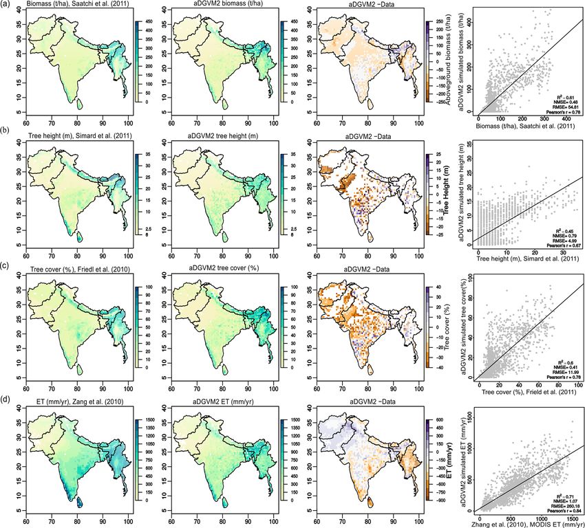
https://doi.org/10.5194/bg-18-2957-2021 Biogeosciences, 18, 2957–2979, 20212968 D. Kumar et al.: Climate change impact on South Asian vegetation Figure 4. Projected change in biomass (t/ha), canopy cover (%) and evapotranspiration (ET, mm/year) between the 2000s and 2050s and between the 2000s and the 2090s under (a) RCP4.5+eCO2 and (b) RCP4.5+f CO2 . See Fig. S7 for projected change of these variables under RCP8.5. Figure 5. Maps showing areas where CO2 fertilization compensates for biomass dieback caused by climate change between the 2000s and the 2090s under (a) RCP4.5 and (b) RCP8.5 and (c) aboveground biomass between 1950 and 2099 for South Asia in different scenarios. Biogeosciences, 18, 2957–2979, 2021 https://doi.org/10.5194/bg-18-2957-2021
D. Kumar et al.: Climate change impact on South Asian vegetation 2969
Table 3. Biome-level ET normalized to biomass (Ebiome , mm/kg/year) for the 2000s, 2050s and 2090s, and percent (%) change in Ebiome
from the 2000s to the 2050s and the 2000s to the 2090s under RCP4.5 and RCP8.5 with fixed and elevated CO2 . 1 indicates percentual ET
changes between time periods.
RCP scenarios Year
C4 grassland
C3 grassland
C4 savanna
C3 savanna
Evg. forest
Dec. forest
Shrubland
Woodland
RCP4.5+f CO2 2010s 186.7 95.5 257 159.7 288.5 183.3 252.5 194.2
2050s 170.9 80.5 217 157.4 291.3 187.2 244.6 151.9
2090s 185 72.3 209.6 140.7 289.3 205.2 247.1 179.1
1 2050s–2010s −8.5 −15.7 −15.6 −1.4 1 2.1 −3.1 −21.8
1 2090s–2010s −0.9 −24.3 −18.5 −11.9 0.3 11.9 −2.1 −7.8
RCP4.5+eCO2 2010s 185.4 93.4 259.7 159.7 288.1 190.9 251.6 188.4
2050s 161.2 79.7 217 147.8 283 183.2 238.2 153.4
2090s 164.1 73.4 210.2 138.7 280.4 197.2 236.6 157.1
1 2050s–2010s −13.1 −14.6 −16.5 −7.4 −1.8 −4.1 −5.3 −18.6
1 2090s–2010s −11.5 −21.4 −19.1 −13.2 −2.7 3.3 −6 −16.6
RCP8.5+f CO2 2010s 172.8 87.4 257.5 160.9 286.5 185.5 244.7 188.1
2050s 153.7 72.7 243.2 158.3 298.5 195.1 241 162.7
2090s 195.6 67.6 231.1 162.7 301.3 216 267.5 150.2
1 2050s–2010s −11.1 −16.8 −5.5 −1.6 4.2 5.2 −1.5 −13.5
1 2090s–2010s 13.2 −22.6 −10.2 1.1 5.2 16.4 9.3 −20.1
RCP8.5+eCO2 2010s 177.5 91.1 256.4 162.7 284.5 192.5 243.7 191.7
2050s 143.9 76.9 235.6 149.4 285.4 184.6 228.8 153.1
2090s 141.4 59.2 218.3 143.9 284.9 186 242.3 143.2
1 2050s–2010s −18.9 −15.6 −8.1 −8.1 0.3 −4.1 −6.1 −20.1
1 2090s–2010s −20.3 −35.1 −14.9 −11.6 0.1 −3.4 −0.6 −25.3
The deciduous behavior is advantageous in dry regions, as the IBIS model also predicted transitions toward evergreen
in the Deccan region, because trees that do not invest much forest.
carbon into their leaves per unit dry mass (higher ASLA and Woody encroachment in many ecosystems is attributed to
lower LL) lose less investment when shedding them dur- rising CO2 , and this is supported by studies based on both
ing the dry season. Phenology change as a result of climate field observations (e.g., FACE experiments) and satellite data
change has already been observed (Buitenwerf et al., 2015; (Brienen et al., 2015; Fischlin et al., 2007; Piao et al., 2006;
Cleland et al., 2007). In Scheiter et al. (2020), we showed that Schimel et al., 2015; Archer et al., 2017; Stevens et al.,
climate change supports transitions to tall evergreen vegeta- 2017). The aDGVM2 also supports these findings, i.e., in-
tion in tropical Asia and found increases in the abundance of creasing canopy cover and woody biomass under the eCO2
evergreen plants and decreases in the abundance of decid- condition, and agrees with the reported greening trend in
uous plants in mainland Southeast Asia, central India and South Asia during the last three decades (Wang et al., 2017).
Pakistan. This relative advantage of evergreen plants over Elevated CO2 affects plants by increasing their photosyn-
deciduous plants under elevated CO2 in aDGVM2 can be thetic rate, growth rate and water use efficiency, leading to
explained by the fact that increased intrinsic water use ef- an increase in biomass (Leakey et al., 2009; Norby and Zak,
ficiency under eCO2 in evergreen plants is higher than in de- 2011). Increased photosynthetic rates under elevated CO2
ciduous plants as demonstrated by Soh et al. (2019). Previ- are due to an increase in the rate of rubisco carboxylation
ous modeling studies also support aDGVM2 result showing for C3 plants, with a concurrent decrease in photorespira-
transitions from deciduous to evergreen vegetation. With the tory losses of carbon (Long et al., 2004). Due to the im-
BIOME4 model, Ravindranath et al. (2006) simulated the re- proved carboxylation efficiency, C3 plants can respond by
sponse of forest to Special Report on Emissions Scenarios reducing stomatal conductance, thereby reducing transpira-
(SRES) A2 and B2 and reported similar changes toward ev- tional losses, improving leaf water status and water use ef-
ergreen phenology. A study by Chaturvedi et al. (2011) using ficiency, and favoring leaf area growth (Long et al., 2004;
Norby and Zak, 2011). Evidence from both observation and
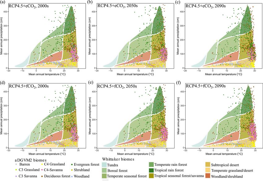
https://doi.org/10.5194/bg-18-2957-2021 Biogeosciences, 18, 2957–2979, 20212970 D. Kumar et al.: Climate change impact on South Asian vegetation Figure 6. Relationship between (a) evapotranspiration (ET) and mean annual precipitation (MAP), (b) ET and mean annual temperature (MAT), (c) mean aboveground biomass and MAP, and (d) mean aboveground biomass and MAT under RCP4.5. The lines (both solid and dotted) in all figures represent the best-fit regression line. Data points represent spatially averaged ET (a, b) and biomass (c, d) over all of South Asia for each year from 1950 to 2099. See Fig. S8 for results under RCP8.5. modeling of forest dynamic suggests that combined effects rer et al. (2019) showed that the global-scale response to of eCO2 and increased water use efficiency include increases eCO2 from experiments is similar to past changes in green- in forest growth and canopy greening, as well as widespread ness (Piao et al., 2019) and biomass (Sitch et al., 2015) in increases in woody plant biomass and potential forest car- response to eCO2 . This suggests that CO2 will likely con- bon sink. However, it is still unclear how the CO2 responses tinue to stimulate plant biomass in the future despite the con- scale to the ecosystem level (Hickler et al., 2015) and how straining effect of soil nutrients; however Terrer et al. (2019) nutrient limitation from the soil may influence ecosystem re- also argued that the empirical relationships with soil nutrients sponses to eCO2 . Körner (2015) argued that carbon from the can be powerful for explaining large-scale patterns of eCO2 atmosphere can only be converted into biomass if other fac- responses, despite ecosystem-level uncertainties. According tors such as nutrients, temperature and water are not limit- to our simulations we can conclude that natural vegetation ing. In addition, the benefit of eCO2 can be downregulated of South Asia likely will remain a carbon sink in the future by broad-scale forest die-off due to frequent drought and (Fig. 5). warmer temperature (Choat et al., 2018; Mcdowell et al., 2016), as well as tree mortality due to negative tree physi- 4.2 Impact of climate change and fixed CO2 on biomes ological responses, negative carbon balance and accelerated and biomass pest attacks. Rising background mortality rates combined with projected increases in intensity, frequency and duration Under both f CO2 scenarios, the spatial distribution of sa- of drought (Huang et al., 2016) increase the uncertainty re- vanna areas remained in its contemporary state. Central In- garding positive effects of eCO2 . dia and the Deccan Plateau showed a transition of deciduous In the long run, whether ecosystems act as a carbon source forest to savanna, because forest canopy opened up due to or sink can be estimated using models that consider all fac- tree mortality caused by increasing temperature and reduced tors that are relevant in the carbon cycle and its associated MAP. This indicates that plants experience temperature and factors (Fatichi et al., 2014; Körner, 2015). However, Ter- drought stress under fixed CO2 . These stresses were compen- Biogeosciences, 18, 2957–2979, 2021 https://doi.org/10.5194/bg-18-2957-2021
You can also read